
Chapter | three
Digital Representation
CHAPTER OUTLINE
Lower fs and Fewer Bits per Sample
How Much Space Does (Linear) Digital Audio Take Up?
Digital audio technology is based on the transformation of a signal varying in an analog manner to numerical values at an appropriate rate. After this conversion, computers can be used in the processing, transmission, and storage of the signals.
Other advantages of digital audio technology include error correction, which allows for the execution of copying and transmission in a lossless manner. In addition it enables what otherwise would have to be done with physical components such as resistors, capacitors, and inductors to now be represented as simple calculations.
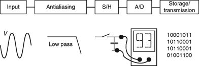
FIGURE 3.1 Principles for the digitizing of analog signals. The signal is low-pass filtered before a sampling of the signal is performed. The magnitude (quantization) of each sample is then determined. The resolution is determined by the number of bits.
ANTIALIASING
Before the analog signal can be converted to a digital signal, it is necessary to determine a well-defined upper cut-off frequency (fu), and a low-pass filter is used for this. This filtering is called antialiasing; the term “alias” means an assumed identity. The necessity of the filtering is due to the sampling process itself. The analog signal must not contain frequencies that are higher than half of the sampling frequency (a frequency also called the Nyquist frequency). If the sampling frequency is lower than twice the highest input frequency, then the reconstructed signal will contain frequency components that were not present in the original. The filter ensures that the signal does not contain any aliasing frequencies after reconstruction.
SAMPLING
After the low-pass filtering, sampling is performed. Sampling consists of measuring the instantaneous value of the signal. The frequency at which this measurement is taken is called the sampling frequency (fs).
A comparison can be made with a movie camera that can record moving pictures by taking a single picture 24 times per second. One could then say that the camera’s sampling frequency is 24 Hz. Now and then you can also observe alias frequencies elsewhere, such as when we see the wheels of the stagecoach turning backwards while the horses and the carriage are moving forward.
Sampling frequencies of 32 kHz, 44.1 kHz, and 48 kHz have long been the standard for quality audio for things like CD or broadcast audio tracks. However, the use of 88.2 kHz, 96 kHz, 176.4 kHz, and 192 kHz has gradually also become commonplace. The latter are seen in use particularly with DVD and Blu-ray audio tracks.
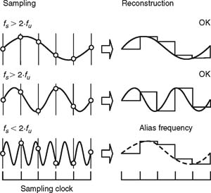
FIGURE 3.2 If the sampling frequency is not at least twice the highest audio frequency the reconstructed signal will not be in accordance with the input.
Sound clips for computer games, audio in communication systems, and other similar types of audio typically use very low sampling frequencies down to 8 kHz or even less.
For each sample, the instantaneous value of the analog signal is retained for as long as the analog to digital converter (also called an A-D converter or ADC) needs to perform its conversion. In the early converters this was performed by a “hold” circuit, which fundamentally was a capacitor that was charged/discharged to the instantaneous value of the signal at the point in time the sample was taken. The reading of the analog signal in modern converters occurs so quickly that the hold function can be omitted. However, the understanding of the sampling process is easier when keeping a “virtual capacitor” in mind.
Oversampling, sampling done at a frequency that is a number of times higher than the requisite minimum, is performed in many converters. Oversampling is utilized because it makes it easier to implement antialiasing filters. In addition, oversampling is a necessity when the signal must be resolved into many bits, again because it is not possible to implement filters that are as sharp as would be needed to, for example, be able to make a difference at a resolution of 24 bits.
The SACD (Super Audio Compact Disc) uses oversampling providing a direct stream of data that requires a sampling frequency 64 times that of the standard CD and ends up with a sampling frequency of 2.8224 MHz.
QUANTIZATION
Now comes the part of the process that determines the digital “number.” This process is called quantization. The word comes from Latin (quantitas = size). During quantization, the size of the individual sample is converted to a number. This transformation, or conversion, is not always completely ideal, however.
The scale that is being used for purposes of comparison has a finite resolution that is determined by the number of bits. The word “bit” is a contraction of the words “binary digit,” which refers to a digit in the binary number system. With quantization, it is the number of bits that determine the precision of the value read. Each time there is one more bit available, the resolution of the scale is doubled and so the error in measurement is halved. In practice, this means that the signal-to-noise ratio is improved by approx. 6 dB for each extra bit that is available.
BINARY VALUES
The value ascribed to the quantization is not a decimal number but, rather, a binary number. The binary number system uses the number 2 as its base number. This means that only two numbers are available, namely 0 and 1. These values are easy to create and detect in electrical terms. For example, there is a voltage (1), or there is not a voltage (0); the current is running in one direction (1), or the current is running in the opposite direction (0).
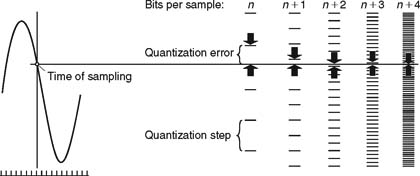
FIGURE 3.3 With quantization, it is the number of bits that determine the precision of the value read. Each time there is one more bit available, the resolution of the scale is doubled and the error in measurement is halved. In practice this means that the signalto- noise ratio is improved by approximately 6 dB for each extra bit that is available.
With one digit, or one bit, available we thus only have two values, namely 0 and 1. With two bits available, we have four possible combinations, namely 00 (zero, zero), 01 (zero, one), 10 (one, zero) and 11 (one, one). The number of steps on the scale equals the number of bits to the power of two. In practice, between 8 and 24 bits are used in the quantization of analog signals. CDquality audio corresponds to 16 bits per sample (= 162 = 65,536 possible values). There are only a finite number of values available when the magnitude of the signal is determined. This means that the actual analog value at the moment of sampling is in fact represented by the nearest value on the scale.
With linear quantization (equal distance between the quantization steps), a resolution of only a few bits would result in extreme distortion of the original signal. When it is resolved with additional bits, this distortion gradually becomes something that can be perceived as broadband noise. As a rule of thumb, the signal-to-noise ratio is estimated to be about 6 dB per bit.
A-D
The principal components in the A-D converter are one or more comparators, which compare the instantaneous values of the individual samples with a built-in voltage reference. After the comparison, the comparator’s output will indicate the value 0 (or “low”) if the signal’s instantaneous value is less than the reference. If the signal’s instantaneous value is equal to or greater than the reference, then the output of the comparator will indicate the value 1 (or “high”).
For serial (sequential) quantization, the comparator will first determine the most significant bit, and then the next bit, etc. until the least significant bit has been determined. For a parallel conversion, a comparator is required for each level that is to be determined, which for n bits corresponds to 2n-l. If, for example, there are eight bits available for the total signal, this corresponds to a resolution of 256 levels, represented by numerical values in the range 0-255. Written in binary format, this corresponds to the numbers from 00000000 to 11111111. A form of encoding is normally used where the first digit specifies the polarity of the signal. If the number is 0 then a positive voltage value has been sampled. If the number is 1, then a negative voltage value has been sampled.
Many converters have been designed according to the Delta-Sigma principle. This uses oversampling with a frequency so high that it only needs to be determined for each sample whether the current value is greater or smaller than the prior value. The advantage is that errors can only arise of a magnitude corresponding to that of the smallest quantization interval, whereas the errors in parallel conversion can be much greater. After the conversion, the long sequence of serial information can be reorganized into a standard parallel bit format at a standardized sampling frequency, so that it can be used for CD, DAT, etc. For SACD, the bit stream (Direct Stream Digital or DSD) generated by the Delta-Sigma converter is what is recorded.
Some converter types combine parallel and serial conversion (Flash converter), where four or five bits are typically determined at a time. This combines high speed with good precision.
D-A
In the conversion from digital to analog, the objective is to produce a signal that is proportional to the value that is contained in the numerical digital information. This can be done in principle by having each bit represent a voltage source such that the most significant bit is converted into the largest voltage, the next most significant bit is converted into half of that voltage, etc. All of the voltage steps are added, and a holding circuit ensures that the signal is continuous until the next sample has been reestablished. The signal created is then smoothed out by the use of a low-pass filter.

FIGURE 3.4 During digital-to-analog conversion, the stored numbers are converted back to an analog signal. The numbers are essentially read into a programmable power supply, so that they re-create the corresponding voltage steps. The low-pass filter smoothes out the signal by removing the harmonic overtones (caused by the steps) lying above the desired frequency spectrum.
The D-A conversion is in principle quite simple; however it can be difficult to control in the real world, where for example 216 = 65,536 different levels could be generated for a 16-bit signal. There can certainly be differences in the quality of A-D converters in practice. Poor converters can have a DC offset and poor linearity in their dynamics. Methods exist however, to reduce these problems.
BIT REDUCTION
The quality of digital sound can in principle be determined by the number of bits per sample and by the sampling frequency. In both cases, the higher the better. The problem is that for many purposes, transmitting sound over the Internet, storage for handheld devices, etc., it is not possible to transfer the number of bits per seconds required for high-quality audio (i.e., CD, SACD, DVD, Blu-ray) within a reasonable amount of time.
Therefore some compromise must be introduced, such as the number of bits per second being lowered. This is called bit reduction or bit companding (a mixture of the words compressing and expanding). Fundamentally, there are a number of different methodologies available.
Lossless Packing
One principle for reducing the number of bits does not actually throw any information away. One system is known as MLP, Meridian Lossless Packing. This is equivalent to zipping a data file. The information is packed so it takes up less space but the contents are still intact. Another system is FLAC, Free Lossless Audio Codec. which is very popular due to its fast decoding. As it is a nonproprietary format several codecs are available. The store data are reduced to approximately half size.
Lower fs and Fewer Bits per Sample
The simplest method is to use a lower sampling frequency and fewer bits per sample; however, this results in deterioration in quality.
Nonlinear Quantization
A method that has been used for many years is nonlinear quantization. with specificially the A-law (telephony in Europe) and m-law (mu-law, telephony in the US) methods being the most widely used variants. These require only 8 bits per sample but effectively give 12 bits of resolution basically obtained by fine resolution at low levels and an increasingly more coarse resolution as levels gets higher. This method is often used in communications; however, the quality is not good enough for music.
Perceptual Coding
The dominating methodology is called perceptual coding, and is based on psycho acoustics. It makes use of the fact that the ear does not necessarily hear everything in a complex spectrum. Strong parts of the spectrum mask weaker parts. The principle is then that what is not audible can be discarded. (Read more about masking in Chapter 7.)
For perceptual coding, a frequency analysis is performed. One single sample by itself has no frequency information; hence a greater number of samples are collected, typically 1024. Calculations are then performed from frequency band to frequency band determining whether signals in the surrounding parts of the frequency spectrum are masking precisely this band. The data in bands that are masked are more or less thrown away. In addition, multiple channels can share information they have in common. Bits are only used in those ranges that are most important for the sequence concerned. Depending on the algorithms used the contents may be reduced to a few percent of the original size.
One of the drawbacks of all these methodologies is that it takes time to compress the bit stream and it takes time to expand it again. Time delays of up to a few hundred milliseconds will be experienced in the transmissions, solely due to the complexity of the algorithms. With perceptually coded signals, another problem can arise when any kind of signal processing is applied. The thresholds that might have kept the artifacts at an audible minimum suddenly may change and have an influence on the sound quality perceived.
Codecs and Applications
There are an overwhelming number of bit reduction algorithms available. Some are initiated by standards organizations while others are proprietary company standards. The different methods are in general optimized for different applications like download and storage for personal playback devices, Internet media, VoIP, video embedded audio, digital broadcast, etc. Often new algorithms are based on older versions and may or may not be backward compatible. This is an area of constant development. So the following compressed overview in Table 3.1 can be regarded as a snapshot providing information on a few currently widely used algorithms.
TABLE 3.1 The Most Popular Non-Proprietary Formats for Perceptually Coded Audio.

HOW MUCH SPACE DOES (LINEAR) DIGITAL AUDIO TAKE UP?
When calculating the size of any digital information handled by computers one has to be aware that it is all based on bytes [B], which each contain 8 bits. This is why the number of bits per sample is calculated as an integer times the number 8 (1·8, 2·8, 3·8, etc). The number of bits per sample of linear PCM (Pulse Code Modulation, digital audio) is basically 8 (1 byte), 16 (2 bytes), 24 (3 bytes), or 32 (4 bytes). For internal processing 64 bits or more can be used.
Because these numbers get large the use of prefixes gets very handy. Here we use “k” (kilo), “M” (Mega), “G” (Giga), “T” (Tera), etc. The sizes are calculated as follows:
1 kB = 1024 B = 8192 bits
1 MB = 1024 kB = 8,388,608 bits (z 8.39·106 bits)
1 GB = 1024 MB z 8.59·109 bits
1 TB = 1024 GB z 8.8·1012 bits
Example:
How much storage capacity is needed for a 1-hour stereo recording in 44.1 kHz/16 bit?
The total number of bits is calculated as follows:
Sampling frequency·no. of bits per sample·no. of audio channels·the duration of the recording:
44,100 (samples per second)·16 (bits per sample)·2 (channels)·1 (hour)·
60 (minutes)·60 (seconds) = 5.08·109 bits
Number of bytes: 5.08·109/8 = 6.35·108 B
Number of kB: 6.35·108/1024 = 6.20·105 kB
Number of MB: 6.20·105/1024 = 605.6 MB
This is in the range of the storage capacity for a CD. For this example, additional data such as the file header and table of contents, is not taken into consideration.