Distance vector
</objective> <objective>Link state
</objective> <objective>Administrative distance
</objective> <objective></objective> <objective></objective> </feature><feature><title>Concepts and Techniques You’ll Need to Master:</title> <objective>Configuring EIGRP
</objective> <objective>Configuring OSPF
</objective> </feature>In Chapter 10, “Basic Routing,” you learned about static, default, and RIP routing. These are good solutions for small networks but do not scale well. Static routing becomes prone to errors and is cumbersome to do on a large scale, default routing does not help in getting to various networks within an enterprise, and RIP routing has a maximum hop count limitation of fifteen hops. For larger networks you need a scalable solution. Two good solutions are the Enhanced Interior Gateway Protocol (EIGRP) and the Open Shortest Path First (OSPF) routing protocols.
EIGRP is a hybrid routing protocol developed by Cisco to replace IGRP. It uses the Diffusing Update Algorithm (DUAL) developed by Dr. J. J. Garcia-Luna-Aceves. Similar to RIP, it has a maximum hop count, but its maximum is 224. Unlike RIP, however, it does not send out periodic updates. Instead, EIGRP sends updates only when there is a change in the network.
EIGRP uses the bandwidth and delay of an interface by default, with the option of factoring reliability, load, and MTU. EIGRP maintains three tables, as shown in Figure 14.1:
Neighbor table
Topology table
Routing table
EIGRP begins by sending HELLO packets out all active interfaces. The router listens for HELLO packets from other routers. From the HELLO packets, the router learns of neighboring routers, which get listed in the neighbor table. After the router knows of its neighbors, it begins exchanging routes with its neighbors. These routes go into the topology table, which is similar to a routing table, but no decision has been made yet as to the best route. Instead, the topology table is used to build a map of the network with different speed limits (bandwidth) on the different roads (links). The DUAL algorithm is run against the topology table, and two routes are determined as a result:
Successor route—. This is the best route as determined by the DUAL algorithm. This route gets injected into the routing table and is the one used when packets are routed.
Feasible successor route—. This is the next best route and is kept in the topology table. It is used only in the event that the primary successor route goes down.
By having a feasible successor route, the router is ready to instantly inject another route into the routing table should the successor ever go down. This makes convergence very rapid with EIGRP.
In addition to being a rapidly converging protocol, EIGRP is the only routing protocol that supports multiple Layer 3 protocols, namely IP, AppleTalk, and IPX. All the other routing protocols mentioned in this chapter support only IP. EIGRP maintains separate tables for each of the three protocols it supports.
Another distinction of EIGRP is its use of two administrative distance values. EIGRP uses administrative distance 90 for routes learned through EIGRP. Routes can also be redistributed into EIGRP from another routing protocol. When this occurs, redistributed routes get an administrative distance of 170. Internal routes are best described as those that are direct testimony, or trusted the most, whereas external routes are like hearsay and are therefore trusted less.
Exam Alert
Remember the main characteristics of EIGRP:
Hybrid protocol
Supports IP, AppleTalk, and IPX
Has two administrative distance values, one for internal and one for external (redistributed routes)
Uses bandwidth and delay by default in calculating its metric, but can also factor reliability, load, and MTU
Basic EIGRP configuration is not that different from configuring RIP. The primary difference for basic configuration is that you must specify an autonomous system number that defines your routing domain. The autonomous system number is assigned globally for the routing process and can be any number you want, but that same number must be used on all routers. Routing updates will not be exchanged between routers with different autonomous numbers. Because the exam focuses heavily on troubleshooting, make sure you always check that the autonomous numbers match in the exam scenarios.
The following example shows how to configure EIGRP for a router connected to networks 192.168.10.0/24 and 192.168.20.0/24. The autonomous system number is 1 and is specified when entering the routing process.
Router(config)#router eigrp 1
Router(config-router)#network 192.168.10.0
Router(config-router)#network 192.168.20.0
Similar to RIP version 2 and OSPF, EIGRP can be a classless routing protocol. By default, it is classful. To enable classless routing, type the following command under the routing process:
Router(config-router)#no auto-summaryA good engineer does not just configure routing but knows to verify the configuration with show commands. The most common show command when verifying your routing configuration is show ip route. This command was discussed in Chapter 10, so it is not discussed here. Keep in mind, though, that this is best command to use to see whether your routing table is being populated.
You can use other commands besides show ip route to verify your EIGRP configuration. These include show ip protocols and show ip eigrp topology.
The first command, show ip protocols, is helpful to see your autonomous system number and the networks you are advertising.
Router# show ip protocols
Routing Protocol is "eigrp 1"
  Outgoing update filter list for all interfaces is not set
  Incoming update filter list for all interfaces is not set
  Redistributing: eigrp 1
  Automatic network summarization is in effect
  Routing for Networks:
    192.168.0.0
  Routing Information Sources:
    Gateway         Distance      Last Update
    192.168.1.0          90      0:02:36
    192.168.2.0          90      0:03:04
    192.168.3.0          90      0:03:04
  Distance: internal 90 external 170
Table 14.1 summarizes the important lines of this command.
Table 14.1. Summary of Show IP Protocols Output
Output | Description |
|---|---|
Outgoing/incoming filters | Used to filter routing updates between routers. |
Redistributing | Covered in the Cisco Certified Network Professional (CCNP) exam. This pertains to redistributing information between routing protocols and is outside the scope of this exam. |
Automatic network summarization is in effect | Whether the |
Routing for networks | Which networks your router is advertising to other routers. |
Routing information sources | This defines which routers are sending your EIGRP routes, the administrative distance for those routes, and the last time your router received an update from other routers. |
Distance | The administrative distance for internal and external routes. |
The second command is show ip eigrp topology. As the command suggests, this outputs your topology table. Your topology table contains all the routes your router knows about. Here is where you will also see your successor (best routes) and your feasible successor (backup routes):
Router# show ip eigrp topology

IP-EIGRP Topology Table for process 77

Codes: P - Passive, A - Active, U - Update, Q - Query, R - Reply,
       r - Reply status

P 172.16.0.0 255.255.0.0, 2 successors, FD is 36251776
          via 172.16.17.1 (36251776/36226176), Ethernet0
          via 172.16.18.1 (36251776/36226176), Ethernet1
P 172.20.0.0 255.255.0.0, 1 successors, FD is 307200
          via 172.16.81.28 (307200/281600), Ethernet1
          via 172.16.19.5 (702311/295210), Ethernet2
From this output you can begin to get an idea of the topology of your network. Notice that for the 172.16.0.0/16 network you have two successors. This is because the metric is the same for both networks and, subsequently, you will load balance across two networks. The metric that is put in the routing table is the first number in parenthesis (36251776 in this example) and is called the feasible distance (FD).
The 172.20.0.0 network has only one successor route out Ethernet1 that is learned from a router with the IP address 172.16.81.28. You also have a backup route (feasible successor) out Ethernet2 that is learned from a router at 172.16.19.5.
For the exam, make sure you are comfortable analyzing the output of these show commands.
Another scalable routing protocol is the Open Shortest Path First (OSPF) protocol. OSPF was developed by the Internet Engineering Task Force (IETF) in 1988 as a more scalable solution than RIP. Unlike EIGRP, OSPF is an open standard and is not Cisco proprietary. It uses the Shortest Path First (SPF) algorithm developed by Edgar Dijkstra. It is a link state routing protocol, which means that it sends updates only when there is a change in the network, and instead of sending routing updates, it sends link state advertisements (LSAs) instead.
OSPF is a polite protocol. Unlike chatty RIP, which broadcasts out its entire routing table every 30 seconds regardless of whether other routers want to hear it, OSPF takes a more gentlemanlike approach to routing. First, OSPF sends out hello messages to neighboring routers to announce itself as an OSPF router and discover who its neighbor routers are. Routers have to agree on certain parameters (such as timers and being on a common subnet) before they can become neighbors. After its neighbor routers are discovered, they begin to exchange information about networks (links) it knows about, using messages called link state advertisements (LSAs). After exchanging all routes, the routers send out updates only when there is a change, and they send information only for that affected route, not the entire routing table. Routers take the link state advertisements heard from other routers and place those routes in its link state database (similar to the topology database in EIGRP). Routers then run the SPF algorithm to determine the best route to a destination and place that route in the routing table.
To determine the best path, OSPF uses a metric called cost, which Cisco defines as 108/bandwidth. If you had a 100Mbps link, the cost would be 1 because 100,000,000/100,000,000. Here are some other common costs:
10Mbps: 10
1.544Mbps (T1): 64
64Kbps: 1562
Exam Alert
These examples are not included just to impress you with the authors’ math abilities. You should know the formula to determine the cost of a link. Given the bandwidth of an interface, know how to calculate the OSPF cost.
The bandwidth costs are based on a bandwidth reference of 100Mb. If you have faster links in your enterprise, such as Gigabit Ethernet, you can change what OSPF bases its cost on by using the auto-cost reference bandwidth command. For example, to change your OSPF to use 109/bandwidth (1,000,000 or GB), type the following command under the router process configuration mode:
Router(config-router)#auto-cost reference-bandwidth 1000000To maintain consistency throughout your network, you should set the same bandwidth reference across on all your routers.
The SPF algorithm places each router as the “root” of a tree and calculates the shortest path from itself to each destination. The shortest path then gets put into the routing table and is used to route packets to their destination.
An important concept to grasp with OSPF is that it is a hierarchical protocol. Hierarchical routing protocols break up your autonomous system into multiple areas and summarize routes between areas. If summarized wisely, you can cut down a significant portion of routing updates by advertising only the summarized route.
As the number of networks increases in your domain, the amount of processing required on each router increases. To lower the amount of processing required, you can use route summarization. Route summarization looks for the same sequence of bits used in subnetworks and creates a less-explicit summary route. For example, Figure 14.2 shows four networks in area 2:
172.16.0.0/24
172.17.0.0/24
172.18.0.0/24
172.19.0.0/24
The first octet, 172, is the same for all four routes, but the second octet differs. By looking for similar bits, we can create a single summary route:
128 | 64 | 32 | 16 | 8 | 4 | 2 | 1 | |
|---|---|---|---|---|---|---|---|---|
16 | 0 | 0 | 0 | 1 | 0 | 0 | 0 | 0 |
17 | 0 | 0 | 0 | 1 | 0 | 0 | 0 | 1 |
18 | 0 | 0 | 0 | 1 | 0 | 0 | 1 | 0 |
19 | 0 | 0 | 0 | 1 | 0 | 0 | 1 | 1 |
The bits are the same up to the 4-bit position. Only the 16-bit position is set to 1, so by ignoring the last two bits (because they change), we are left with 172.16.0.0. The subnet mask has changed, however, because we are no longer working with a /24. Instead, our subnet mask has moved two places to the left because the last two bit positions vary for the four networks. Our resulting summarized route is 172.16.0.0/22 (255.255.252.0). This will be the route that gets injected into area 0 from area 2.
The routers in area 0 and area 1 have to process only the one summarized route instead of four individual routes. Being able to summarize your routes between areas provides several benefits:
Less processing on routers—. This is not only because of the single network statement (in contrast to four), but also because of the lack of recalculation should a more specific network (that is, a /24) go down.
Instability hidden from other routers—. If a single network goes down in area 2, it will not affect the routers in area 0 and area 1.
Fast convergence—. Because fewer routes are sent to area 0, the routers in areas 0 and 1 can converge faster.
Less bandwidth overhead—. There is less bandwidth because only one route is sent, so the advertisement is smaller.
Greater control over routing updates—. Because you gain control over routing updates, you can control what routes get sent from one area to another.
You might have noticed that both area 2 and area 1 are connected via area 0. Area 0 is the “backbone” area in OSPF, and all other areas must be connected to it. Routes are then summarized into your backbone area.
Summarizing is an excellent way to conserve your precious bandwidth. On networks that contain more than two routers, OSPF can also conserve bandwidth by electing a designated router for that network that all routers communicate with. Routers exchange information with a designated router instead of each other. This cuts down significantly on the number of advertisements.
The process of using a designated router is somewhat complex, so let’s go through it one step at a time. First, the designated router (DR) is elected on only two types of networks:
Broadcast multi-access—. Ethernet, Token Ring
Nonbroadcast multi-access—. Frame Relay, ATM, X.25
On a point-to-point network with only two routers, there is no need for this type of election. Remember that on a point-to-point network, there is no point (of having a DR).
Second, the DR is not the only type of router elected on these types of networks. A backup designated router (BDR) is used in the event that a DR should fail.
The DR and BDR election is as follows:
The router with the highest priority becomes the DR. The router with the second-highest priority becomes the BDR. Priority is a number between 0 and 255 and is configured on an interface with the command
ip ospf_prioritypriority_number. The default priority is 1, and if the router is set to priority 0, it will never become a DR or BDR.In the case of a tie, such as when every router’s priority is left to the default of 1, the tie breaker is the router with the highest router ID.
Every router has an identifier called a router ID (RID) that is used to identify itself in its messages. The router ID is an IP address and is assigned as follows:
The router ID can be configured with the
router-idcommand under the OSPF routing process. You can choose a valid IP address that you are using on the router or make up a new one.If the
router-idcommand is not used, the numerically highest IP address on any loopback interface is chosen as the router ID. A loopback interface is a virtual, software-only interface that never goes down.If you do not have any loopback interfaces configured, the highest IP address on any active physical interface is chosen as the router ID.
See if you can spot the router ID given the following IP addresses on a router:
Serial 0/0: 192.168.100.19
FastEthernet 0/0: 10.0.0.1
Loopback 0: 172.16.201.200
Although the highest IP address is the one configured on the serial interface, a loopback interface takes precedence over any physical interfaces. Therefore, the router ID would be 172.16.201.200.
Exam Alert
The router-id command is common in the real world, but for the test, make sure that you know the process the router uses to select a router ID if the router-id command is not used. It first looks at the highest IP address on any logical (loopback) interface, and if no loopback interfaces exist, it looks at the highest IP address on any active physical interface.
Let’s review. On broadcast and nonbroadcast multi-access networks, a designated router and backup designated router are elected. The election is done by first choosing the routers with the highest priority value or, if the priorities are same, choosing the routers with the highest router ID. The router ID is chosen by the highest IP address on any loopback interface or, if no loopback interfaces are configured, the highest IP address on any active physical interface. Whew! That’s a lot of work, but in the end it will conserve a significant amount of bandwidth by minimizing the number of link state messages.
Now that we have elected a DR and BDR, the next phase is ready to begin. In Figure 14.3, you see five routers. The Mocha router is the DR, and the Latte router is the BDR. Instead of all routers sending link state advertisements to each other, they send out messages only to the DR and BDR. Messages are sent to the multicast address of 224.0.0.6; both the DR and BDR belong to this multicast group address.
Next, the Mocha router, which is the DR, takes the information it learned from the other routers and sends it back out to all routers, as shown in Figure 14.4. Messages are sent to the AllSPFRouter multicast address of 224.0.0.5; all routers running OSPF are members of this multicast group address.
Understanding the complexities involved in OSPF is the difficult part; configuring it is fairly straightforward. The process is the same as with the other protocols. First, we enable the routing protocol. This is done with the command router ospf <process-id>. The process ID can be any number you prefer between 1 and 65,535. Note that this is not the same as the autonomous system number found in IGRP and EIGRP. Here, the process ID is local to the router and does not need to match other routers.
The next step is to activate OSPF on your interfaces and advertise your networks. This is done with the network command as before, but the syntax is a little different. Here, the syntax is
network network address wild card mask area area-id
Note that you specify a wildcard mask in the configuration. Wildcard masks are covered in Chapter 13, “IP Access Lists.” Here, wildcard masks are used to match the IP address that is being used on an interface.
Take a look at Figure 14.5, where we come across our three friends again: Moe, Larry, and Curly. Given this example, the configuration for Moe would be
Moe(config)#router ospf 1
Moe(config-router)#network 192.168.10.0 0.0.0.255 area 0
Moe(config-router)#network 192.168.20.0 0.0.0.255 area 0
Larry’s configuration would be
Larry(config)#router ospf 1
Larry(config-router)#network 192.168.20.0 0.0.0.255 area 0
Larry(config-router)#network 192.168.40.0 0.0.0.255 area 1
Finally, Curly’s configuration would be
Curly(config)#router ospf 1
Curly(config-router)#network 192.168.40.0 0.0.0.255 area 1
Curly(config-router)#network 192.168.50.0 0.0.0.255 area 1
The wildcard mask used in these statements is matching the IP address on the interface. Here, we are matching the entire network, of which the IP address is a part. For example, on Curly’s router, the command network 192.168.40.0 0.0.0.255 area 1 tells the router to match all addresses that begin with 192.168.40. The last octet, which has 255 in the wildcard mask, is ignored. The router examines the IP addresses of its directly connected interfaces and activates OSPF on those interfaces that match the statement.
Because you are using wildcard masks to match the IP address on your directly connected interfaces, you could also use the wildcard mask of 0.0.0.0 to match the exact address. Just as with IP access lists in Chapter 13, a wildcard mask of 0.0.0.0 would match a specific address. For example, if Curly had the IP address of 192.168.40.1 on one interface and 192.168.50.1 on another interface, you could configure Curly’s router using a wildcard mask of 0.0.0.0:
Curly(config)router ospf 1
Curly(config-router)#network 192.168.40.1 0.0.0.0 area 1
Curly(config-router)#network 192.168.50.1 0.0.0.0 area 1
Using a wildcard mask that matches the IP address of the interface is equivalent to using a wildcard mask that matches the network where the IP address resides. For the exam, focus on matching the entire network (0.0.0.255 wildcard mask in the previous example); the reasons behind which one you should choose are outside the scope of this book and, for that matter, the exam.
Exam Alert
The syntax for OSPF is slightly different from other routing protocols. Make sure that you feel comfortable configuring OSPF. Remember, it uses a process ID, not an autonomous system. Also, OSPF uses wildcard masks and not subnet masks in its configuration.
There are two optional commands that you should be familiar with for the CCNA exam. These commands, configured under the interface, are
ip ospf prioritypriority_number—This is used to change the priority of an interface for the DR/BDR election.ip ospf costcost—This is used to manually change the cost of an interface.
For verification, you can use the show ip protocols and show ip route as before. Other commands you can use to verify your configuration are
show ip ospf interface—This command displays area ID and DR/BDR information.show ip ospf neighbor—This command displays neighbor information.
You can use the debug ip ospf events command to troubleshoot OSPF. This command is helpful to troubleshoot why routers are not forming a neighbor relationship with each other. Similar to EIGRP, OSPF routers form neighbor relationships before exchanging any routing information. Several items must line up, however, for a neighbor adjacency to be established:
Timers must be the same on both routers. OSPF uses hello timers that define how often they send out hello messages and dead timers that define how long after a router stops hearing a Hello message does it declare its neighbor as down.
Interfaces connecting the two routers must be in the same area.
Password authentication, if being used, must be the same.
Type of area must be the same. (This last item is outside the scope of the CCNA test, but it is covered on the CCNP BSCI exam.)
Neighbors are formed automatically or can be established through the use of the neighbor command done under the routing process. Sometimes the neighbor adjacency does not form, and the debug ip ospf events command can help you to troubleshoot what is going wrong. The following debug output shows an example of an adjacency not forming because of two routers having different timers configured:
Router#debug ip ospf events
OSPF: hello with invalid timers on interface FastEthernet0/0
hello interval received 10 configured 10
netmask received 255.255.0.0 configured 255.255.0.0
dead interval received 40 configured 60You are working in an environment that is running IP, IPX, and AppleTalk. What routing protocol inherently supports all three of these protocols? | |||||||||||
How is the router ID chosen in OSPF? Select all that apply. | |||||||||||
Examine the following figure. What routing protocol can you use to accommodate the given addressing scheme? Select all that apply. | |||||||||||
OSPF supports hierarchical routing. What benefits do you gain from using a routing protocol that supports hierarchical routing? Select all that apply.
| |||||||||||
What is the cost of a 128K link in OSPF? | |||||||||||
You have a serial interface with the IP address of 192.168.22.33/30. How would you add this link to area 0 in the OSPF process? | |||||||||||
Which of the following protocols maintains a topology table? For questions 8–10 refer to the following figure and configuration. | |||||||||||
What is wrong with the Botswana configuration? | |||||||||||
What is wrong with the Ukraine configuration? | |||||||||||
What is wrong with the Tanzania configuration? |