It is important to follow a few rules and guidelines when summarizing. Serious routing problems will happen otherwise—such as routers advertising networks inaccurately and possibly duplicating other routers’ advertisements, sub-optimal or even totally incorrect routing, and severe data loss.

The first rule is to design your networks with summarization in mind, even if you don’t need it yet. This means that you will group contiguous subnets together behind the router that will summarize them—you do not want to have some subnets from a summarized group behind some other router. The summary is essentially saying, “I can reach the networks represented by this summary; send any traffic for them through me.” If one (or more) of the networks behind the summarizing router is unavailable, traffic will be dropped—but not by the summarizing router, because the summary is still valid. The packet will get routed to the router that connects to the dead network, and dropped there. Advance planning, including making plenty of room for future growth, will give you a solid, scalable network design that readily lends itself to summarizing. Figure 16.4 shows a badly designed network that will be almost impossible to summarize because the subnets are discontiguous, with individual subnets scattered all over the system.

Figure 16.4. Poor planning prevents proper performance.

The second rule is to summarize into the core of your network. The core is where the bigger, faster, busier routers are—like the Central Office router in the previous example. These routers have the job of dealing with high volumes of traffic headed for all different areas of the network, so we do not want to burden them with big, highly detailed route tables. The further you get from the core, the more detail the routers need to get traffic to the correct destination network. It’s much like using a map to drive to a friend’s house; you don’t need a great deal of detail when you are on the highway, but when you get into the residential areas, you need to know very precise information if you have a hope of finding the place.

Figure 16.5 illustrates the same network after your friendly neighborhood Cisco Certified Internetwork Expert has spent the afternoon readdressing the network and configuring summarization. This network will scale beautifully and have minimal performance issues (at least because of route table and routing update overhead).

Figure 16.5. Proper planning prevents poor performance.

Following these rules will give you one of the additional benefits of summarization as well: hiding instability in the summarized networks. Let’s say that one of the branches is having serious spanning-tree problems because an MCP was allowed to configure a Cisco switch. (This is actually a felony in some states.) That route could be “flapping”—up, down, up, down—as spanning-tree wreaks havoc with your network. The router will be doing its job, sending out updates every time the route flaps. If we were not summarizing, those flapping messages would propagate through the entire corporate system, putting a totally unnecessary and performance-robbing load on the routers. Once you summarize, the summary is stable: It can’t flap because it is not a real network. It’s just like a spokesperson at a press conference: “The rumors of a fire at the Springfield plant have had no impact on production whatsoever.” Meanwhile, the Springfield plant could be a charred hulk. The summary is still valid, and traffic will still be sent to the router connected to the flapping network. This keeps people from asking any more questions about the Springfield fire... however, if someone were to send a shipment to Springfield, it would be hastily redirected to another site (or dropped). All we have done is hide the problem from the rest of the world, so we don’t flood the Net with rapid-fire routing updates.

When using classless routing protocols, creating summary addresses is a totally manual process. Classful routing protocols perform automatic summarization, but that is not as fancy as it sounds. They simply treat any subnet as the classful address from which it was created, which works if your networks are built with this in mind; however, in reality that is too simplistic and real networks need more customized summarization. The upshot of all this is that you need to understand how to determine the summary address given a set of networks to be summarized, and you also need to be able to figure out if a particular network is included in a given summary.

Remember that summarization is exactly the opposite of subnetting; in fact, another term for summarization is supernetting. (You might also see it called aggregation.) When we subnet, we lengthen the mask, doubling the number of networks each time we add an extra bit to the mask. Supernetting does the opposite: For each bit we retract or shorten the mask, we combine networks into groups that follow the binary increment numbers.

To illustrate this, let’s look at the private Class B address space. These networks are listed as follows:

172.16.0.0 /16

172.17.0.0 /16

172.18.0.0 /16

172.19.0.0 /16

172.20.0.0 /16

172.21.0.0 /16

172.22.0.0 /16

172.23.0.0 /16

172.24.0.0 /16

172.25.0.0 /16

172.26.0.0 /16

172.27.0.0 /16

172.28.0.0 /16

172.29.0.0 /16

172.30.0.0 /16

172.31.0.0 /16

If you look carefully, you will notice that the range of networks is identified in the second octet. The octet where the range is happening is referred to as the interesting octet. This is your first clue where to begin your summarization.

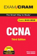
The next step is to figure out what the binary values of the network’s range are. The binary values for the interesting octet are shown in Figure 16.6.

You should see a pattern in the binary values: The first four bits are all the same. The range is actually happening in the last four bits in the second octet; those four bits range from 0000 through 1111; the first four bits are common for all 16 networks in the range.

The next step is to identify those common bits. While you are learning how to do this, it’s a good idea to write out the binary for the range and draw a line that represents the boundary between the common bits and the variable bits in the range. Remember, be absolutely sure that your boundary line is in the right place: For all the networks in the range, everything to the left of the line must be identical, and everything to the right will be the ranging values.

The next step is easy. We are about to summarize: All we need to do is to build a subnet mask that puts a 1 under all of the common bits in the range, and a 0 under everything else—ones to the left of the boundary, and zeroes to the right, as shown in Figure 16.7.

Figure 16.7. Identifying and masking the common bits in a summary.

The last step is to actually create the summary statement. A summary is always an IP address plus a mask; the IP is usually a NetID, and it should be the first network in the range. In our example, the first NetID is 172.16.0.0 so that is the IP we will use. For the mask, the first octet is the same in the whole range, and we have figured out that the first four bits in the second octet are always the same. Remembering that a mask is always a string of 1s followed by a string of 0s, this means that we should mask all eight bits in the first octet and the first four in the second octet, so our mask looks like this:

11111111.11110000.00000000.00000000

That can also be expressed as

255.240.0.0 or /12

So, our summary statement becomes

172.16.0.0 255.240.0.0

or

172.16.0.0 /12

Reverse engineering this is the same process. You are given a summary statement and asked what networks it includes. The octet in which the mask changes from 1s to 0s is the interesting one, where the range will be defined. Jot down the address and mask in that octet in binary and see what possible values are in the range. Then check the networks to see if those are in the range. Figure 16.8 gives an example.

Figure 16.8. Summary address analysis.

If a router learns of two routes to a given network, say one from RIP and one from OSPF, the routing information source with the lowest administrative distance (AD) will be chosen and used. RIP has an AD of 120, and OSPF has an AD of 110. OSPF, therefore, is more trusted as a source of routing information, and the route learned from OSPF will be installed in the route table.

In all but a few exceptional cases (notably with some static route implementations), the router cannot install a route in the route table unless the next-hop address specified by that route is valid. In other words, if the device to which traffic destined for a particular network must be sent is not available, the route is invalid and will be dropped from the route table.

Given that we might learn more than one route to a given network from any one protocol, the router distinguishes between these routes by comparing the metrics. A metric is a measurement of how good a particular route is, expressed as a number. Each routing protocol uses different metrics and different algorithms to calculate them as you saw in Chapter 10, “Basic Routing.” The simple rule is: The lower the metric, the better the route. If two routes have equal metrics, more than one route can be used at a time. (The router will load balance using all routes equally.)

The Longest Match rule is the criterion that a router will use to determine the best route given a choice between two or more that are very similar. The longest match refers to the longest prefix length, or the longest matching string of bits in the route as compared to the destination address of the packet being routed.

The concept behind this rule is very simple: The longer the match in the prefix, the more detailed the route is. Let us look at an example to clarify; Figure 16.9 shows a simplified output of the IP route table:

Assume that a packet has arrived at the router with a destination IP of 172.16.10.131. The router examines its IP route table and discovers that there are five entries in the route table. The entries are sorted per network according to the length of the mask for that network.

The first entry (172.16.0.0 /24) is compared to the destination IP of the packet. The /24 in the route table entry specifies that the first 24 bits of the prefix should be compared for the longest match. Because the destination IP of the packet is 172.16.10.131, the first 24 bits do not match, and this entry is not a possible route for this packet.

The router repeats the process for the remaining four entries. The second, third, and fourth entries all match for their respective prefix lengths of /28, /26, and /24. The fifth entry is a default route, which by definition matches any address, but with a /0 prefix length.

So now the router must decide which entry is the best route to use for the packet in question. All of the entries are valid, but the one with the longest prefix length match—172.16.10.128 /28—is chosen as the best. The default route is a poor match in this case because there are other, more precise routes with longer prefix matches.

Having made its routing decision, the router switches the packet out the Ethernet 0 interface and begins processing the next packet.

An organization called the Internet Corporation for Assigned Network Numbers (ICANN) has the overall responsibility for dividing up the IPv6 address space. They do so with the benefit of a better understanding of the global demand for Internet IP addresses and the luxury of a huge number of addresses to hand out.

The system works like this: First, remember that for the Internet to work well, we need to use route summarization so that the route tables don’t get huge and slow the routers down. Route summarization works best if every router is responsible only for its “branch of the tree,” with smaller branches feeding into larger and larger ones as we get closer to the core or trunk of the tree. This allows the possibility for a single router to advertise a summary that in effect says, “I can reach all North American routes.” That big router connects to other routers that summarize routes for four major Internet service providers (ISPs). Each ISP router connects to smaller ISPs or large enterprise customers, who advertise the summaries that represent the addresses assigned to them. Figure 16.10 gives some idea of how this system works.

Figure 16.10. Global IPv6 address design.

The beauty of the system is that it is organized, planned, and executed in advance, with efficient routing in mind. The large number of addresses available also means that changes at or below the ISP level, for example, because of mergers or large customers changing Internet providers, do not affect the global routing information at the core.

IPv6 addresses are different in appearance from IPv4. Of course, they are 128 bits long, so even in binary they would be four times longer than a 32-bit IPv4 address, but in notation that humans read and write the format is still different. Instead of using dotted decimal in four octets, we use hexadecimal in eight sets of four characters separated by colons, like this:

2201:0FA0:080B:2112:0000:0000:0000:0001

The use of hex makes it a little easier to represent all those 128 bits in a shorter format because each character represents 4 bits. But it’s still a long thing to type out, and remember that network people are generally lazy—so we have a couple of truncation methods to make the long addresses even shorter. The first method is that we are allowed to drop leading zeros—zeros that appear at the beginning of each set, like so:

2201:FA0:80B:2112:0:0:0:1

That makes for a little less typing and a little more clarity. Pay attention to the fact that dropping zeros at the end of each set is not allowed! Dropping leading zeros does not change the value of the set; dropping zeros at the end does (like removing a zero from the end of your paycheck amount—not good!)

The second truncation method we can use is to condense contiguous groups of all-zero sets. In our example, there are three sets that are all zeros. We can represent these by a double colon, like this:

2201:FA0:80B:2112::1

This is as short as it gets. We are only allowed to do the double-colon trick once in any address, so if you see an address with two double-colons in it, it is not valid. Here’s an example:

2201::BCBG::1

One last piece of the addressing notation: the mask. We do not represent the mask as another set of hex characters; instead, we identify the prefix length with slash notation. This is not as confusing at it seems: the slash notation simply identifies how many bits identify the network part, with the remainder being the host part.

As an example, the North American registry ARIN (American Registry for Internet Numbers) was given the block of 2620:0000::/23 in September 2006. This indicates that the first 23 bits of 2620:0000:: identify the block of addresses that the North American routers will advertise to the rest of the world. From this point, ARIN will assign chunks of that space to the Big ISPs; Big ISP1 might get 2620:0100::/24, and Big ISP2 might get 2620:0200::/24. Those ISPs then hand out pieces of their chunk to smaller ISP or big customers, and the prefix length will get bigger as the chunks gets smaller—this should feel familiar because what we are doing here is subnetting. Don’t worry, you won’t be expected to subnet in IPv6. Not yet at least...

An IPv6 address will be one of the following three types. Some will be familiar, but there is one brand-new one, too.

There is no such thing as a broadcast in IPv6. Ever. Any requirement for broadcasting is performed by a multicast instead.

For hosts to use IPv6 addresses, an IPv6 protocol stack must be installed. This likely means that you will need to upgrade your router IOS to provide IPv6 support. Then you can choose one of four options for address assignment.

To understand the address assignment choices better, we need to examine the concepts of stateful versus stateless configuration and the EUI-64 address format.

In IPv6, we can use DHCP to assign IP addresses just like in IPv4. The admin must set up the server with a scope of IPv6 addresses to hand out. The mechanisms used to discover and assign addresses are a little different, but the net result is the same. This is called stateful addressing, where the DHCP server keeps track of what hosts have been assigned what IPv6 address—in other words, the state of the host DHCP-wise.

There is another option for dynamic addressing in IPv6 called stateless autoconfiguration. This feature allows a host to choose and configure an address for itself. The host that wants an address learns what the /64 network prefix is on the local link, then appends its MAC address (in a special 64-bit format called EUI-64), thus generating a 128-bit IPv6 address that is unique to that host because it incorporates the unique MAC of the host.

The EUI-64 format is not so difficult to understand. We simply take the 48-bit MAC address and put a special pattern, FFFE, after the first 24 bits (the six OUI characters), followed by the rest of the six hex characters in the host MAC. The only trick is that according to IPv6 rules, the seventh bit in an EUI-64 address must be 1, which identifies that the burned-in MAC address has been modified. This is a little confusing, to be sure, but you can relax because the host determines and configures its EUI-64 address all by itself, if you tell it to. Here’s what an EUI-64 address conversion looks like:

Original MAC:

00-15-C5-CB-42-2B

Original MAC in binary:

00000000-00010101-11000101-11001011-01000010-00101011

7^th bit = 0

Change 7^th bit to 1:

00000010-00010101-11000101-11001011-01000010-00101011

EUI-64 MAC now:

02-15-C5-CB-42-2B

EUI-64 Address = </64 net_ID_variable>:0215:C5FF:FECB:422B

So, back to the four choices. The following really simplifies the options:

Assuming your IOS provides IPv6 support, giving it an IPv6 address is really easy. The command is carried out at the interface configuration prompt:

interface fastethernet 1/0
ipv6 address 2001:AB00:00FF:1::/64 eui-64

Notice the eui-64 switch; this tells the router to figure out its own EUI-64 address to follow the /64 prefix provided. Without that, you must provide a full 128-bit address in the command.

To verify your configuration, use the show ipv6 interface command at the interface configuration prompt. The following is a sample output (with different addresses applied). You can see multiple addresses in use by the interface for global unicast, link-local, and multiple multicast groups:

Router#show ipv6 interface
  Serial1/0 is up, line protocol is up
    IPv6 is enabled, link-local address is FE80::A8BB:CCFF:FE00:D200
    Global unicast address(es):
      2001:1:33::3, subnet is 2001:1:33::/64 [TENTATIVE]
    Joined group address(es):
      FF02::1
      FF02::1:FF00:3
      FF02::1:FF00:D200
    MTU is 1500 bytes
    ICMP error messages limited to one every 100 milliseconds
    ICMP redirects are enabled
    ND DAD is enabled, number of DAD attempts: 1
    ND reachable time is 30000 milliseconds
  Router#

IPv6 has a couple features that you should keep in mind:

As mentioned in the preceding section, the IPv6 header is fixed at 40 bytes (320 bits) in length. Figure 16.11 shows the header fields and their sizes, and this section identifies what the fields are for.

The Version field identifies the IP version of this packet; for IPv6, obviously the version will be 6.

The Traffic Class field is where QoS marking for Layer 3 can be identified. In a nutshell, the higher the value of this field, the more important the packet. Your Cisco routers (and some switches) can be configured to read this value and send a high-priority packet sooner than other lower ones during times of congestion. This is very important for some applications, especially VoIP.

The Flow Label is a number that identifies this packet as one of a flow of packets in a stream from sender to receiver; a good example is a VoIP call. It’s best for VoIP if all the packets in a given call get sent along exactly the same path to the receiving phone, so that they arrive in the same order they were sent. The flow label is one mechanism that IPv6 routers can use to keep track of different application flows and try to make sure that all the packets within a flow get treated the same way.

The Payload Length field indicates how big the payload of this packet is; it can be variable, so the router needs to know where the packet is supposed to end. That way it knows if anything went missing. This is especially important because there is no header checksum, as there used to be in IPv4.

The Next Header field identifies what Layer 4 protocol is in the payload of this packet (same function as the Protocol field in IPv4).

The Hop Limit field is a cool one: Whereas in IPv4 there was a TTL field that limited the life of a packet to 255 hops (the IPv4 TTL value starts at 255 and is decremented by at least 1 as a packet is processed by a router; if it reaches 0, the packet is dropped. This prevents the packet from being endlessly misrouted around the Internet, although it could be misrouted up to 255 hops), IPv6 is smarter: The Hop Limit value is set to the actual number of hops the packet will go through to reach its destination. This hop information comes from the IPv6 routing protocols. The Hop Limit is still decremented by 1 at each router, but the more accurate value means that the packet can’t be misrouted even by one hop.

The Source and Destination Address fields are self-explanatory; remember that the full 128-bit address for each is listed.

Clearly, things are moving toward IPv6. The U.S. government has specified that all federal agencies must deploy IPv6 by 2008. The Peoples Republic of China has a five-year plan for deployment of IPv6 called the China Next Generation Internet. The process, though, is not going to affect every single host in these large networks overnight. Cisco wants you to be aware of their strategies for the transition to using IPv6 while still maintaining IPv4 functionality.

The easiest IPv6 transition choice is called dual stack. Dual stacking means that the host (router, PC, printer, and so on) runs both the IPv4 and IPv6 protocol stacks and can send and receive both types of packets, probably (but not necessarily) on the same interface. The drawbacks here are the additional load on the host and whether an IPv6 stack for that device is available (your old router might not be able to run IPv6).

Tunneling mode creates a tunnel for one protocol through another. You can picture taking an IPv6 packet from the head office, encapsulating it inside an IPv4 packet to transition across the provider network, then decapsulating it on the other side and forwarding the IPv6 packet into the remote branch office. This is known as a 6-to-4 tunnel. These tunnels have a special address range of 2002::/16.

Translation means taking an IPv6 packet, removing the IP header, and replacing it with an IPv4 header that approximates the original IPv6 information as much as possible.

Tunneling is often associated with a NAT router, and sometimes is known as NAT-PT (for Protocol Translation). What happens here is that the IPv6 packet header is removed and replaced with an IPv4 header (or vice versa), effectively changing from one protocol to the other. The big issues with NAT-PT are latency, performance loading, and the loss of header information in the translation process.

You won’t need to actually do any IPv6 configuration for your test, but they might ask you how to do it, or if the config they show you is valid.