Chapter 8. OSPF
This chapter covers the following subjects:
OSPF Fundamentals: This section provides an overview of communication between OSPF routers.
OSPF Configuration: This section describes the OSPF configuration techniques and commands that can be executed to verify the exchange of routes.
Default Route Advertisement: This section explains how default routes are advertised in OSPF.
Common OSPF Optimizations: This section reviews common OSPF settings foroptimizing the operation of the protocol.
The Open Shortest Path First (OSPF) protocol is the first link-state routing protocol covered in this book. OSPF is a nonproprietary Interior Gateway Protocol (IGP) that overcomes the deficiencies of other distance vector routing protocols and distributes routing information within a single OSPF routing domain. OSPF introduced the concept of variable-length subnet masking (VLSM), which supports classless routing, summarization, authentication, and external route tagging. There are two main versions of OSPF in production networks today:
OSPF Version 2 (OSPFv2): Defined in RFC 2328 and supports IPv4
OSPF Version 3 (OSPFv3): Defined in RFC 5340 and modifies the original structure to support IPv6
This chapter explains the core concepts of OSPF and the basics of establishing neighborships and exchanging routes with other OSPF routers. Two other chapters in this book also cover OSPF-related topics. Here is an overview of them:
Chapter 9, “Advanced OSPF”: Explains the function of segmenting the OSPF domain into smaller areas to support larger topologies.
Chapter 10, “OSPFv3”: Explains how OSPF can be used for routing IPv6 packets.
“Do I Know This Already?” Quiz
The “Do I Know This Already?” quiz allows you to assess whether you should read the entire chapter. If you miss no more than one of these self-assessment questions, you might want to move ahead to the “Exam Preparation Tasks” section. Table 8-1 lists the major headings in this chapter and the “Do I Know This Already?” quiz questions covering the material in those headings so you can assess your knowledge of these specific areas. The answers to the “Do I Know This Already?” quiz appear in Appendix A, “Answers to the ‘Do I Know This Already?’ Quiz Questions.”
Table 8-1 “Do I Know This Already?” Foundation Topics Section-to-Question Mapping
Foundation Topics Section |
Questions |
OSPF Fundamentals |
1–3 |
OSPF Configuration |
4–5 |
Default Route Advertisement |
6 |
Common OSPF Optimizations |
7–10 |
1. OSPF uses the protocol number ___________ for its inter-router communication.
87
88
89
90
2. OSPF uses ___________ packet types for inter-router communication.
three
four
five
six
seven
3. What destination addresses does OSPF use, when feasible? (Choose two.)
IP address 224.0.0.5
IP address 224.0.0.10
IP address 224.0.0.8
MAC address 01:00:5E:00:00:05
MAC address 01:00:5E:00:00:0A
4. True or false: OSPF is only enabled on a router interface by using the command network ip-address wildcard-mask area area-id under the OSPF router process.
True
False
5. True or false: The OSPF process ID must match for routers to establish a neighbor adjacency.
True
False
6. True or false: A default route advertised with the command default information-originate in OSPF will always appear as an OSPF inter-area route.
True
False
7. True or false: The router with the highest IP address is the designated router when using a serial point-to-point link.
True
False
8. OSPF automatically assigns a link cost to an interface based on a reference bandwidth of ___________.
100 Mbps
1 Gbps
10 Gbps
40 Gbps
9. What command is configured to prevent a router from becoming the designated router for a network segment?
The interface command ip ospf priority 0
The interface command ip ospf priority 255
The command dr-disable interface-id under the OSPF process
The command passive interface interface-id under the OSPF process
The command dr-priority interface-id 255 under the OSPF process
10. What is the advertised network for the loopback interface with IP address 10.123.4.1/30?
10.123.4.1/24
10.123.4.0/30
10.123.4.1/32
10.123.4.0/24
Answers to the “Do I Know This Already?” quiz:
1 C
2 C
3 A, D
4 B
5 B
6 B
7 B
8 A
9 A
10 C
Foundation Topics
OSPF Fundamentals
OSPF sends to neighboring routers link-state advertisements (LSAs) that contain the link state and link metric. The received LSAs are stored in a local database called the link-state database (LSDB), and they are flooded throughout the OSPF routing domain, just as the advertising router advertised them. All OSPF routers maintain a synchronized identical copy of the LSDB for the same area.
The LSDB provides the topology of the network, in essence providing for the router a complete map of the network. All OSPF routers run the Dijkstra shortest path first (SPF) algorithm to construct a loop-free topology of shortest paths. OSPF dynamically detects topology changes within the network and calculates loop-free paths in a short amount of time with minimal routing protocol traffic.
Each router sees itself as the root or top of the SPF tree (SPT), and the SPT contains all network destinations within the OSPF domain. The SPT differs for each OSPF router, but the LSDB used to calculate the SPT is identical for all OSPF routers.
Figure 8-1 shows a simple OSPF topology and the SPT from R1’s and R4’s perspective. Notice that the local router’s perspective will always be the root (top of the tree). There is a difference in connectivity to the 10.3.3.0/24 network from R1’s SPT and R4’s SPT. From R1’s perspective, the serial link between R3 and R4 is missing; from R4’s perspective, the Ethernet link between R1 and R3 is missing.

Figure 8-1 OSPF Shortest Path First (SPF) Tree
The SPTs give the illusion that no redundancy exists to the networks, but remember that the SPT shows the shortest path to reach a network and is built from the LSDB, which contains all the links for an area. During a topology change, the SPT is rebuilt and may change.
OSPF provides scalability for the routing table by using multiple OSPF areas within the routing domain. Each OSPF area provides a collection of connected networks and hosts that are grouped together. OSPF uses a two-tier hierarchical architecture, where Area 0 is a special area known as the backbone, to which all other areas must connect. In other words, Area 0 provides transit connectivity between nonbackbone areas. Nonbackbone areas advertise routes into the backbone, and the backbone then advertises routes into other nonbackbone areas.
Figure 8-2 shows route advertisement into other areas. Area 12 routes are advertised toArea 0 and then into Area 34. Area 34 routes are advertised to Area 0 and then into Area 12. Area 0 routes are advertised into all other OSPF areas.

Figure 8-2 Two-Tier Hierarchical Area Structure
The exact topology of the area is invisible from outside the area while still providing connectivity to routers outside the area. This means that routers outside the area do not have a complete topological map for that area, which reduces OSPF traffic in that area. When you segment an OSPF routing domain into multiple areas, it is no longer true that all OSPF routers will have identical LSDBs; however, all routers within the same area will have identical area LSDBs.
The reduction in routing traffic uses less router memory and resources and therefore provides scalability. Chapter 9 explains areas in greater depth; this chapter focuses on the core OSPF concepts. For the remainder of this chapter, OSPF Area 0 is used as a reference area.
A router can run multiple OSPF processes. Each process maintains its own unique database, and routes learned in one OSPF process are not available to a different OSPF process without redistribution of routes between processes. The OSPF process numbers are locally significant and do not have to match among routers. Running OSPF process number 1 on one router and running OSPF process number 1234 will still allow the two routers to become neighbors.
Inter-Router Communication
OSPF runs directly over IPv4, using its own protocol 89, which is reserved for OSPF by the Internet Assigned Numbers Authority (IANA). OSPF uses multicast where possible to reduce unnecessary traffic. The two OSPF multicast addresses are as follows:
AllSPFRouters: IPv4 address 224.0.0.5 or MAC address 01:00:5E:00:00:05. All routers running OSPF should be able to receive these packets.
AllDRouters: IPv4 address 224.0.0.6 or MAC address 01:00:5E:00:00:06. Communication with designated routers (DRs) uses this address.
Within the OSPF protocol, five types of packets are communicated. Table 8-2 briefly describes these OSPF packet types.
Table 8-2 OSPF Packet Types
Type |
Packet Name |
Functional Overview |
1 |
Hello |
These packets are for discovering and maintaining neighbors. Packets are sent out periodically on all OSPF interfaces to discover new neighbors while ensuring that other adjacent neighbors are still online. |
2 |
Database description (DBD) or (DDP) |
These packets are for summarizing database contents. Packets are exchanged when an OSPF adjacency is first being formed. These packets are used to describe the contents of the LSDB. |
3 |
Link-state request (LSR) |
These packets are for database downloads. When a router thinks that part of its LSDB is stale, it may request a portion of a neighbor’s database by using this packet type. |
4 |
Link-state update (LSU) |
These packets are for database updates. This is an explicit LSA for a specific network link and normally is sent in direct response to an LSR. |
5 |
Link-state ack |
These packets are for flooding acknowledgments. These packets are sent in response to the flooding of LSAs, thus making flooding a reliable transport feature. |
OSPF Hello Packets
OSPF hello packets are responsible for discovering and maintaining neighbors. In most instances, a router sends hello packets to the AllSPFRouters address (224.0.0.5). Table 8-3 lists some of the data contained within an OSPF hello packet.
Table 8-3 OSPF Hello Packet Fields
Data Field |
Description |
Router ID (RID) |
A unique 32-bit ID within an OSPF domain. |
Authentication options |
A field that allows secure communication between OSPF routers to prevent malicious activity. Options are none, clear text, or Message Digest 5 (MD5) authentication. |
Area ID |
The OSPF area that the OSPF interface belongs to. It is a 32-bit number that can be written in dotted-decimal format (0.0.1.0) or decimal (256). |
Interface address mask |
The network mask for the primary IP address for the interface out which the hello is sent. |
Interface priority |
The router interface priority for DR elections. |
Hello interval |
The time span, in seconds, that a router sends out hello packets on the interface. |
Dead interval |
The time span, in seconds, that a router waits to hear a hello from a neighbor router before it declares that router down. |
Designated router and backup designated router |
The IP address of the DR and backup DR (BDR) for the network link. |
Active neighbor |
A list of OSPF neighbors seen on the network segment. A router must have received a hello from the neighbor within the dead interval. |
Router ID
The OSPF router ID (RID) is a 32-bit number that uniquely identifies an OSPF router. In some OSPF output commands, neighbor ID refers to the RID; the terms are synonymous. The RID must be unique for each OSPF process in an OSPF domain and must be unique between OSPF processes on a router.
Neighbors
An OSPF neighbor is a router that shares a common OSPF-enabled network link. OSPF routers discover other neighbors via the OSPF hello packets. An adjacent OSPF neighbor is an OSPF neighbor that shares a synchronized OSPF database between the two neighbors.
Each OSPF process maintains a table for adjacent OSPF neighbors and the state of each router. Table 8-4 briefly describes the OSPF neighbor states.
Table 8-4 OSPF Neighbor States
State |
Description |
Down |
This is the initial state of a neighbor relationship. It indicates that the router has not received any OSPF hello packets. |
Attempt |
This state is relevant to NBMA networks that do not support broadcast and require explicit neighbor configuration. This state indicates that no information has been received recently, but the router is still attempting communication. |
Init |
This state indicates that a hello packet has been received from another router, but bidirectional communication has not been established. |
2-Way |
Bidirectional communication has been established. If a DR or BDR is needed, the election occurs during this state. |
ExStart |
This is the first state in forming an adjacency. Routers identify which router will be the master or slave for the LSDB synchronization. |
Exchange |
During this state, routers are exchanging link states by using DBD packets. |
Loading |
LSR packets are sent to the neighbor, asking for the more recent LSAs that have been discovered (but not received) in the Exchange state. |
Full |
Neighboring routers are fully adjacent. |
Designated Router and Backup Designated Router
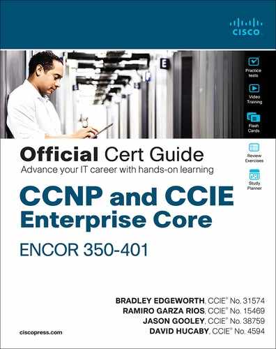
Multi-access networks such as Ethernet (LANs) and Frame Relay allow more than two routers to exist on a network segment. Such a setup could cause scalability problems with OSPF as the number of routers on a segment increases. Additional routers flood more LSAs on the segment, and OSPF traffic becomes excessive as OSPF neighbor adjacencies increase. If four routers share the same multi-access network, six OSPF adjacencies form, along with six occurrences of database flooding on a network. Figure 8-3 shows a simple four-router physical topology and the adjacencies established.
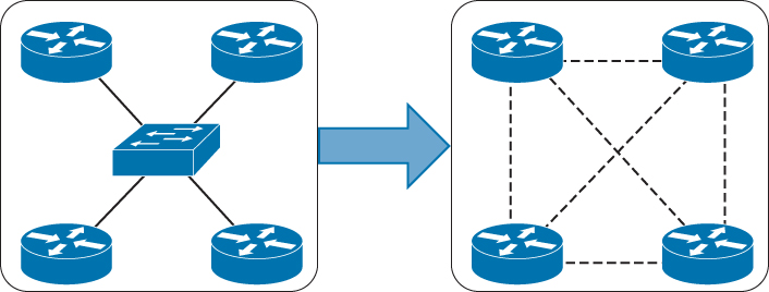
Figure 8-3 Multi-Access Physical Topology Versus Logical Topology
The number of edges formula, n(n – 1) / 2, where n represents the number of routers, is used to identify the number of sessions in a full mesh topology. If 5 routers were present on a segment, 5(5 – 1) / 2 = 10, then 10 OSPF adjacencies would exist for that segment. Continuing the logic, adding 1 additional router would makes 15 OSPF adjacencies on a network segment. Having so many adjacencies per segment consumes more bandwidth, more CPU processing, and more memory to maintain each of the neighbor states.
Figure 8-4 illustrates the exponential rate of OSPF adjacencies needed as routers on a network segment increase.

Figure 8-4 Exponential LSA Sessions for Routers on the Same Segment
OSPF overcomes this inefficiency by creating a pseudonode (virtual router) to manage the adjacency state with all the other routers on that broadcast network segment. A router on the broadcast segment, known as the designated router (DR), assumes the role of the pseudonode. The DR reduces the number of OSPF adjacencies on a multi-access network segment because routers only form a full OSPF adjacency with the DR and not each other. The DR is responsible for flooding updates to all OSPF routers on that segment as the updates occur. Figure 8-5 demonstrates how using a DR simplifies a four-router topology with only three neighbor adjacencies.
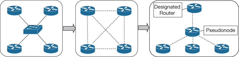
Figure 8-5 OSPF DR Concept
If the DR were to fail, OSPF would need to form new adjacencies, invoking all new LSAs, and could potentially cause a temporary loss of routes. In the event of DR failure, a backup designated router (BDR) becomes the new DR; then an election occurs to replace the BDR. To minimize transition time, the BDR also forms full OSPF adjacencies with all OSPF routers on that segment.
The DR/BDR process distributes LSAs in the following manner:
All OSPF routers (DR, BDR, and DROTHER) on a segment form full OSPF adjacencies with the DR and BDR.
As an OSPF router learns of a new route, it sends the updated LSA to the AllDRouters (224.0.0.6) address, which only the DR and BDR receive and process, as illustrated in step 1 of Figure 8-6.
Figure 8-6 Network Prefix Advertisement with DR Segments
The DR sends a unicast acknowledgment to the router that sent the initial LSA update, as illustrated in step 2 of Figure 8-6.
The DR floods the LSA to all the routers on the segment via the AllSPFRouters (224.0.0.5) address, as shown in step 3 of Figure 8-6.
OSPF Configuration
The configuration process for OSPF resides mostly under the OSPF process, but some OSPF options go directly on the interface configuration submode. The command router ospf process-id defines and initializes the OSPF process. The OSPF process ID is locally significant but is generally kept the same for operational consistency. OSPF is enabled on an interface using two methods:
An OSPF network statement
Interface-specific configuration
The following section describes these techniques.
OSPF Network Statement
The OSPF network statement identifies the interfaces that the OSPF process will use and the area that those interfaces participate in. The network statements match against the primary IPv4 address and netmask associated with an interface.
A common misconception is that the network statement advertises the networks into OSPF; in reality, though, the network statement is selecting and enabling OSPF on the interface. The interface is then advertised in OSPF through the LSA. The network statement uses a wildcard mask, which allows the configuration to be as specific or vague as necessary. The selection of interfaces within the OSPF process is accomplished by using the command network ip-address wildcard-mask area area-id.
The concept is similar to the configuration of Enhanced Interior Gateway Routing Protocol (EIGRP), except that the OSPF area is specified. If the IP address for an interface matches two network statements with different areas, the most explicit network statement (that is, the longest match) preempts the other network statements for area allocation.
The connected network for the OSPF-enabled interface is added to the OSPF LSDB under the corresponding OSPF area in which the interface participates. Secondary connected networks are added to the LSDB only if the secondary IP address matches a network statement associated with the same area.
To help illustrate the concept, the following scenarios explain potential use cases of the network statement for a router with four interfaces. Table 8-5 provides IP addresses and interfaces.
Table 8-5 Table of Sample Interfaces and IP Addresses
IOS Interface |
IP Address |
GigabitEthernet0/0 |
10.0.0.10/24 |
GigabitEthernet0/1 |
10.0.10.10/24 |
GigabitEthernet0/2 |
192.0.0.10/24 |
GigabitEthernet0/3 |
192.10.0.10/24 |
The configuration in Example 8-1 enables OSPF for Area 0 only on the interfaces that explicitly match the IP addresses in Table 8-4.
Example 8-1 Configuring OSPF with Explicit IP Addresses
router ospf  1
    network 10.0.0.10 0.0.0.0 area 0
    network 10.0.10.10 0.0.0.0 area 0
    network 192.0.0.10 0.0.0.0 area 0
    network 192.10.0.10 0.0.0.0 area 0
Example 8-2 displays the OSPF configuration for Area 0, using network statements that match the subnets used in Table 8-4. If you set the last octet of the IP address to 0 and change the wildcard mask to 255, the network statements match all IP addresses within the /24 network.
Example 8-2 Configuring OSPF with Explicit Subnet
router ospf  1
    network 10.0.0.0 0.0.0.255 area 0
    network 10.0.10.0 0.0.0.255 area 0
    network 192.0.0.0 0.0.0.255 area 0
    network 192.10.0.0 0.0.0.255 area 0
Example 8-3 displays the OSPF configuration for Area 0, using network statements for interfaces that are within the 10.0.0.0/8 or 192.0.0.0/8 network ranges, and will result in OSPF being enabled on all four interfaces, as in the previous two examples.
Example 8-3 Configuring OSPF with Large Subnet Ranges
router ospf  1
    network 10.0.0.0 0.255.255.255 area 0
    network 192.0.0.0 0.255.255.255 area 0
Example 8-4 displays the OSPF configuration for Area 0 to enable OSPF on all interfaces.
Example 8-4 Configuring OSPF for All Interfaces
router ospf  1
    network 0.0.0.0 255.255.255.255 area 0
Interface-Specific Configuration
The second method for enabling OSPF on an interface for IOS is to configure it specifically on an interface with the command ip ospf process-id area area-id [secondaries none]. This method also adds secondary connected networks to the LSDB unless the secondaries none option is used.
This method provides explicit control for enabling OSPF; however, the configuration is not centralized and increases in complexity as the number of interfaces on the routers increases. If a hybrid configuration exists on a router, interface-specific settings take precedence over the network statement with the assignment of the areas.
Example 8-5 provides a sample interface-specific configuration.
Example 8-5 Configuring OSPF on IOS for a Specific Interface
interface GigabitEthernet 0/0
    ip address 10.0.0.1 255.255.255.0
    ip ospf 1 area
Statically Setting the Router ID
By default, the RID is dynamically allocated using the highest IP address of any up loopback interfaces. If there are no up loopback interfaces, the highest IP address of any active up physical interfaces becomes the RID when the OSPF process initializes.
The OSPF process selects the RID when the OSPF process initializes, and it does not change until the process restarts. Interface changes (such as addition/removal of IP addresses) on a router are detected when the OSPF process restarts, and the RID changes accordingly.
The OSPF topology is built on the RID. Setting a static RID helps with troubleshooting and reduces LSAs when a RID changes in an OSPF environment. The RID is four octets in length but generally represents an IPv4 address that resides on the router for operational simplicity; however, this is not a requirement. The command router-id router-id statically assigns the OSPF RID under the OSPF process.
The command clear ip ospf process restarts the OSPF process on a router so that OSPF can use the new RID.
Passive Interfaces
Enabling an interface with OSPF is the quickest way to advertise a network segment to other OSPF routers. However, it might be easy for someone to plug in an unauthorized OSPF router on an OSPF-enabled network segment and introduce false routes, thus causing havoc in the network. Making the network interface passive still adds the network segment into the LSDB but prohibits the interface from forming OSPF adjacencies. A passive interface does not send out OSPF hellos and does not process any received OSPF packets.
The command passive interface-id under the OSPF process makes the interface passive, and the command passive interface default makes all interfaces passive. To allow for an interface to process OSPF packets, the command no passive interface-id is used.
Requirements for Neighbor Adjacency
The following list of requirements must be met for an OSPF neighborship to be formed:
RIDs must be unique between the two devices. They should be unique for the entire OSPF routing domain to prevent errors.
The interfaces must share a common subnet. OSPF uses the interface’s primary IP address when sending out OSPF hellos. The network mask (netmask) in the hello packet is used to extract the network ID of the hello packet.
The MTUs (maximum transmission units) on the interfaces must match. The OSPF protocol does not support fragmentation, so the MTUs on the interfaces should match.
The area ID must match for the segment.
The DR enablement must match for the segment.
OSPF hello and dead timers must match for the segment.
Authentication type and credentials (if any) must match for the segment.
Area type flags must match for the segment (for example, Stub, NSSA). (These are not discussed in this book.)
Sample Topology and Configuration
Figure 8-7 shows a topology example of a basic OSPF configuration. All four routers have loopback IP addresses that match their RIDs (R1 equals 192.168.1.1, R2 equals 192.168.2.2, and so on).

Figure 8-7 Sample OSPF Topology
On R1 and R2, OSPF is enabled on all interfaces with one command, R3 uses specific network-based statements, and R4 uses interface-specific commands. R1 and R2 set the Gi0/2 interface as passive, and R3 and R4 make all interfaces passive by default but make Gi0/1 active.
Example 8-6 provides a sample configuration for all four routers.
Example 8-6 Configuring OSPF for the Topology Example
! OSPF is enabled with a single command, and the passive interface is
! set individually
R1# configure terminal
Enter configuration commands, one per line. End with CNTL/Z.
R1(config)# interface Loopback0
R1(config-if)# ip address 192.168.1.1 255.255.255.255
R1(config-if)# interface GigabitEthernet0/1
R1(config-if)# ip address 10.123.4.1 255.255.255.0
R1(config-if)# interface GigabitEthernet0/2
R1(config-if)# ip address 10.1.1.1 255.255.255.0
R1(config-if)#
R1(config-if)# router ospf 1
R1(config-router)# router-id 192.168.1.1
R1(config-router)# passive-interface GigabitEthernet0/2
R1(config-router)# network 0.0.0.0 255.255.255.255 area 0
! OSPF is enabled with a single command, and the passive interface is
! set individually
R2(config)# interface Loopback0
R2(config-if)# ip address 192.168.2.2 255.255.255.255
R2(config-if)# interface GigabitEthernet0/1
R2(config-if)# ip address 10.123.4.2 255.255.255.0
R2(config-if)# interface GigabitEthernet0/2
R2(config-if)# ip address 10.2.2.2 255.255.255.0
R2(config-if)#
R2(config-if)# router ospf 1
R2(config-router)# router-id 192.168.2.2
R2(config-router)# passive-interface GigabitEthernet0/2
R2(config-router)# network 0.0.0.0 255.255.255.255 area 0
! OSPF is enabled with a network command per interface, and the passive interface
! is enabled globally while the Gi0/1 interface is reset to active state
R3(config)# interface Loopback0
R3(config-if)# ip address 192.168.3.3 255.255.255.255
R3(config-if)# interface GigabitEthernet0/1
R3(config-if)# ip address 10.123.4.3 255.255.255.0
R3(config-if)# interface GigabitEthernet0/2
R3(config-if)# ip address 10.3.3.3 255.255.255.0
R3(config-if)#
R3(config-if)# router ospf 1
R3(config-router)# router-id 192.168.3.3
R3(config-router)# passive-interface default
R3(config-router)# no passive-interface GigabitEthernet0/1
R3(config-router)# network 10.3.3.3 0.0.0.0 area 0
R3(config-router)# network 10.123.4.3 0.0.0.0 area 0
R3(config-router)# network 192.168.3.3 0.0.0.0 area 0
! OSPF is enabled with a single command under each interface, and the
! passive interface is enabled globally while the Gi0/1 interface is made active.
R4(config-router)# interface Loopback0
R4(config-if)# ip address 192.168.4.4 255.255.255.255
R4(config-if)# ip ospf 1 area 0
R4(config-if)# interface GigabitEthernet0/1
R4(config-if)# ip address 10.123.4.4 255.255.255.0
R4(config-if)# ip ospf 1 area 0
R4(config-if)# interface GigabitEthernet0/2
R4(config-if)# ip address 10.4.4.4 255.255.255.0
R4(config-if)# ip ospf 1 area 0
R4(config-if)#
R4(config-if)# router ospf 1
R4(config-router)# router-id 192.168.4.4
R4(config-router)# passive-interface default
R4(config-router)# no passive-interface GigabitEthernet0/1
Confirmation of Interfaces
It is a good practice to verify that the correct interfaces are running OSPF after making changes to the OSPF configuration. The command show ip ospf interface [brief | interface-id] displays the OSPF-enabled interfaces.
Example 8-7 displays a snippet of the output from R1. The output lists all the OSPF-enabled interfaces, the IP address associated with each interface, the RID for the DR and BDR (and their associated interface IP addresses for that segment), and the OSPF timers for that interface.
Example 8-7 OSPF Interface Output in Detailed Format
R1# show ip ospf interface
! Output omitted for brevity
Loopback0 is up, line protocol is up
  Internet Address 192.168.1.1/32, Area 0, Attached via Network Statement
  Process ID 1, Router ID 192.168.1.1, Network Type LOOPBACK, Cost: 1
  Topology-MTID    Cost    Disabled    Shutdown      Topology Name
        0           1         no          no            Base
  Loopback interface is treated as a stub Host
GigabitEthernet0/1 is up, line protocol is up
  Internet Address 10.123.4.1/24, Area 0, Attached via Network Statement
  Process ID 1, Router ID 192.168.1.1, Network Type BROADCAST, Cost: 1
  Topology-MTID    Cost    Disabled    Shutdown      Topology Name
        0           1         no          no            Bas
  Transmit Delay is 1 sec, State DROTHER, Priority 1
  Designated Router (ID) 192.168.4.4, Interface address 10.123.4.4
  Backup Designated router (ID) 192.168.3.3, Interface address 10.123.4.3
  Timer intervals configured, Hello 10, Dead 40, Wait 40, Retransmit 5
..
  Neighbor Count is 3, Adjacent neighbor count is 2
    Adjacent with neighbor 192.168.3.3  (Backup Designated Router)
    Adjacent with neighbor 192.168.4.4  (Designated Router)
  Suppress hello for 0 neighbor(s)
Example 8-8 shows the show ip ospf interface command with the brief keyword.
Example 8-8 OSPF Interface Output in Brief Format
R1# show ip ospf interface brief
Interface    PID   Area            IP Address/Mask    Cost  State Nbrs F/C
Lo0          1     0               192.168.1.1/32     1     LOOP  0/0
Gi0/2        1     0               10.1.1.1/24        1     DR    0/0
Gi0/1        1     0               10.123.4.1/24      1     DROTH 2/3
R2# show ip ospf interface brief
Interface    PID   Area            IP Address/Mask    Cost  State Nbrs F/C
Lo0          1     0               192.168.2.2/32     1     LOOP  0/0
Gi0/2        1     0               10.2.2.2/24        1     DR    0/0
Gi0/1        1     0               10.123.4.2/24      1     DROTH 2/3
R3# show ip ospf interface brief
Interface    PID   Area            IP Address/Mask    Cost  State Nbrs F/C
Lo0          1     0               192.168.3.3/32     1     LOOP  0/0
Gi0/1        1     0               10.123.4.3/24      1     BDR   3/3
Gi0/2        1     0               10.3.3.3/24        1     DR    0/0
R4# show ip ospf interface brief
Interface    PID   Area            IP Address/Mask    Cost  State Nbrs F/C
Lo0          1     0               192.168.4.4/32     1     LOOP  0/0
Gi0/1        1     0               10.123.4.4/24      1     DR    3/3
Gi0/2        1     0               10.4.4.4/24        1     DR    0/0
Table 8-6 provides an overview of the fields in the output in Example 8-8.
Table 8-6 OSPF Interface Columns
Field |
Description |
Interface |
Interfaces with OSPF enabled |
PID |
The OSPF process ID associated with this interface |
Area |
The area that this interface is associated with |
IP Address/Mask |
The IP address and subnet mask for the interface |
Cost |
The cost metric assigned to an interface that is used to calculate a path metric |
State |
The current interface state, which could be DR, BDR, DROTHER, LOOP, or Down |
Nbrs F |
The number of neighbor OSPF routers for a segment that are fully adjacent |
Nbrs C |
The number of neighbor OSPF routers for a segment that have been detected and are in a 2-Way state |
Verification of OSPF Neighbor Adjacencies
The command show ip ospf neighbor [detail] provides the OSPF neighbor table. Example 8-9 shows sample output on R1, R2, R3, and R4.
Example 8-9 OSPF Neighbor Output
R1# show ip ospf neighbor
Neighbor ID     Pri   State           Dead Time   Address         Interface
192.168.2.2       1   2WAY/DROTHER    00:00:37    10.123.4.2      GigabitEthernet0/1
192.168.3.3       1   FULL/BDR        00:00:35    10.123.4.3      GigabitEthernet0/1
192.168.4.4       1   FULL/DR         00:00:33    10.123.4.4      GigabitEthernet0/1
R2# show ip ospf neighbor
Neighbor ID     Pri   State           Dead Time   Address         Interface
192.168.1.1       1   2WAY/DROTHER    00:00:30    10.123.4.1      GigabitEthernet0/1
192.168.3.3       1   FULL/BDR        00:00:32    10.123.4.3      GigabitEthernet0/1
192.168.4.4       1   FULL/DR         00:00:31    10.123.4.4      GigabitEthernet0/1
R3# show ip ospf neighbor
Neighbor ID     Pri   State           Dead Time   Address         Interface
192.168.1.1       1   FULL/DROTHER    00:00:35    10.123.4.1      GigabitEthernet0/1
192.168.2.2       1   FULL/DROTHER    00:00:34    10.123.4.2      GigabitEthernet0/1
192.168.4.4       1   FULL/DR         00:00:31    10.123.4.4      GigabitEthernet0/1
R4# show ip ospf neighbor
Neighbor ID     Pri   State           Dead Time   Address         Interface
192.168.1.1       1   FULL/DROTHER    00:00:36    10.123.4.1      GigabitEthernet0/1
192.168.2.2       1   FULL/DROTHER    00:00:34    10.123.4.2      GigabitEthernet0/1
192.168.3.3       1   FULL/BDR        00:00:35    10.123.4.3      GigabitEthernet0/1
Table 8-7 provides a brief overview of the fields shown in Example 8-9. The neighbor states on R1 identify R3 as the BDR and R4 as the DR. R3 and R4 identify R1 and R2 as DROTHER in the output.
Table 8-7 OSPF Neighbor State Fields
Field |
Description |
Neighbor ID |
The router ID (RID) of the neighboring router. |
PRI |
The priority for the neighbor’s interface, which is used for DR/BDR elections. |
State |
The first field is the neighbor state, as described in Table 8-3. The second field is the DR, BDR, or DROTHER role if the interface requires a DR. For non-DR network links, the second field shows just a hyphen (-). |
Dead Time |
The time left until the router is declared unreachable. |
Address |
The primary IP address for the OSPF neighbor. |
Interface |
The local interface to which the OSPF neighbor is attached. |
Verification of OSPF Routes
The next step is to verify the OSPF routes installed in the IP routing table. OSPF routes that install into the Routing Information Base (RIB) are shown with the command show ip route ospf.
Example 8-10 provides sample output of the OSPF routing table for R1. In the output, where two sets of numbers are in the brackets (for example, [110/2]/0, the first number is the administrative distance (AD), which is 110 by default for OSPF, and the second number is the metric of the path used for that network. The output for R2, R3, and R4 would be similar to the output in Example 8-10.
Example 8-10 OSPF Routes Installed in the RIB
R1# show ip route ospf
! Output omitted for brevity
Codes: L - local, C - connected, S - static, R - RIP, M - mobile, B - BGP
       D - EIGRP, EX - EIGRP external, O - OSPF, IA - OSPF inter area
       N1 - OSPF NSSA external type 1, N2 - OSPF NSSA external type 2
       E1 - OSPF external type 1, E2 - OSPF external type 2
Gateway of last resort is not set
      10.0.0.0/8 is variably subnetted, 7 subnets, 2 masks
O        10.2.2.0/24 [110/2] via 10.123.4.2, 00:35:03, GigabitEthernet0/1
O        10.3.3.0/24 [110/2] via 10.123.4.3, 00:35:03, GigabitEthernet0/1
O        10.4.4.0/24 [110/2] via 10.123.4.4, 00:35:03, GigabitEthernet0/1
      192.168.2.0/32 is subnetted, 1 subnets
O        192.168.2.2 [110/2] via 10.123.4.2, 00:35:03, GigabitEthernet0/1
      192.168.3.0/32 is subnetted, 1 subnets
O        192.168.3.3 [110/2] via 10.123.4.3, 00:35:03, GigabitEthernet0/1
      192.168.4.0/32 is subnetted, 1 subnets
O        192.168.4.4 [110/2] via 10.123.4.4, 00:35:03, GigabitEthernet0/1
Default Route Advertisement
OSPF supports advertising the default route into the OSPF domain. The default route is advertised by using the command default-information originate [always] [metric metric-value] [metric-type type-value] underneath the OSPF process.
If a default route does not exist in a routing table, the always optional keyword advertises a default route even if a default route does not exist in the RIB. In addition, the route metric can be changed with the metric metric-value option, and the metric type can be changed with the metric-type type-value option.
Figure 8-8 illustrates a common scenario, where R1 has a static default route to a firewall that is connected to the Internet. To provide connectivity to other parts of the network (for example, R2 and R3), R1 advertises a default route into OSPF.
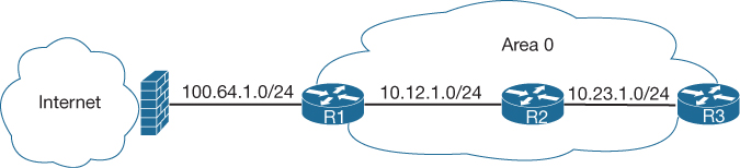
Figure 8-8 Default Route Topology
Example 8-11 provides the relevant configuration on R1. Notice that R1 has a static default route to the firewall (100.64.1.2) to satisfy the requirement of having the default route in the RIB.
Example 8-11 OSPF Default Information Origination Configuration
R1
ip route 0.0.0.0 0.0.0.0 100.64.1.2
!
router ospf 1
 network 10.0.0.0 0.255.255.255 area 0
 default-information originat
Example 8-12 provides the routing tables of R2 and R3. Notice that OSPF advertises the default route as an external OSPF route.
Example 8-12 Routing Tables for R2 and R3
R2# show ip route | begin Gateway
Gateway of last resort is 10.12.1.1 to network 0.0.0.0

O*E2  0.0.0.0/0 [110/1] via 10.12.1.1, 00:02:56, GigabitEthernet0/1
      10.0.0.0/8 is variably subnetted, 4 subnets, 2 masks
C        10.12.1.0/24 is directly connected, GigabitEthernet0/1
C        10.23.1.0/24 is directly connected, GigabitEthernet0/2
R3# show ip route | begin Gateway
Gateway of last resort is 10.23.1.2 to network 0.0.0.0
O*E2  0.0.0.0/0 [110/1] via 10.23.1.2, 00:01:47, GigabitEthernet0/1
      10.0.0.0/8 is variably subnetted, 3 subnets, 2 masks
O        10.12.1.0/24 [110/2] via 10.23.1.2, 00:05:20, GigabitEthernet0/1
C        10.23.1.0/24 is directly connected, GigabitEthernet0/
Common OSPF Optimizations
Almost every network requires tuning based on the equipment, technical requirements, or a variety of other factors. The following sections explain common concepts involved with the tuning of an OSPF network.
Link Costs
Interface cost is an essential component of Dijkstra’s SPF calculation because the shortest path metric is based on the cumulative interface cost (that is, metric) from the router to the destination. OSPF assigns the OSPF link cost (that is, metric) for an interface by using the formula in Figure 8-9.
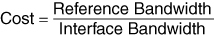
Figure 8-9 OSPF Interface Cost Formula
The default reference bandwidth is 100 Mbps. Table 8-8 provides the OSPF cost for common network interface types using the default reference bandwidth.
Table 8-8 OSPF Interface Costs Using Default Settings
Interface Type |
OSPF Cost |
T1 |
64 |
Ethernet |
10 |
FastEthernet |
1 |
GigabitEthernet |
1 |
10 GigabitEthernet |
1 |
Notice in Table 8-8 that there is no differentiation in the link cost associated with a FastEthernet interface and a 10 GigabitEthernet interface. Changing the reference bandwidth to a higher value allows for a differentiation of cost between higher-speed interfaces. Making the value too high could cause issues because low-bandwidth interfaces would not be distinguishable. The OSPF LSA metric field is 16 bits, and the interface cost cannot exceed 65,535.
Under the OSPF process, the command auto-cost reference-bandwidth bandwidth-in-mbps changes the reference bandwidth for all OSPF interfaces associated with that process. If the reference bandwidth is changed on one router, the reference bandwidth should be changed on all OSPF routers to ensure that SPF uses the same logic to prevent routing loops. It is a best practice to set the same reference bandwidth for all OSPF routers.
The OSPF cost can be set manually with the command ip ospf cost 1–65535 underneath the interface. While the interface cost is limited to 65,535 because of LSA field limitations, the path metric can exceed a 16-bit value (65,535) because all the link metrics are calculated locally.
Failure Detection
A secondary function of the OSPF hello packets is to ensure that adjacent OSPF neighbors are still healthy and available. OSPF sends hello packets at set intervals, based on the hello timer. OSPF uses a second timer called the OSPF dead interval timer, which defaults to four times the hello timer. Upon receipt of a hello packet from a neighboring router, the OSPF dead timer resets to the initial value and then starts to decrement again.
If a router does not receive a hello before the OSPF dead interval timer reaches 0, the neighbor state is changed to down. The OSPF router immediately sends out the appropriate LSA, reflecting the topology change, and the SPF algorithm processes on all routers within the area.
Hello Timer
The default OSPF hello timer interval varies based on the OSPF network type. OSPF allows modification to the hello timer interval with values between 1 and 65,535 seconds. Changing the hello timer interval modifies the default dead interval, too. The OSPF hello timer is modified with the interface configuration submode command ip ospf hello-interval 1–65535.
Dead Interval Timer
The dead interval timer can be changed to a value between 1 and 65,535 seconds. The OSPF dead interval timer can be changed with the command ip ospf dead-interval 1–65535 under the interface configuration sub mode.
Verifying OSPF Timers
The timers for an OSPF interfaces are shown with the command show ip ospf interface, as demonstrated in Example 8-13. Notice the highlighted hello and dead timers.
Example 8-13 OSPF Interface Timers
R1# show ip ospf interface | i Timer|line
Loopback0 is up, line protocol is up
GigabitEthernet0/2 is up, line protocol is up
  Timer intervals configured, Hello 10, Dead 40, Wait 40, Retransmit 5
GigabitEthernet0/1 is up, line protocol is up
  Timer intervals configured, Hello 10, Dead 40, Wait 40, Retransmit 5
DR Placement
The DR and BDR roles for a broadcast network consume CPU and memory on the host routers in order to maintain states with all the other routers for that segment. Placing the DR and BDR roles on routers with adequate resources is recommended.
The following sections explain the DR election process and how the DR role can be assigned to specific hardware.
Designated Router Elections
The DR/BDR election occurs during OSPF neighborship—specifically during the last phase of 2-Way neighbor state and just before the ExStart state. When a router enters the 2-Way state, it has already received a hello from the neighbor. If the hello packet includes a RID other than 0.0.0.0 for the DR or BDR, the new router assumes that the current routers are the actual DR and BDR.
Any router with OSPF priority of 1 to 255 on its OSPF interface attempts to become the DR. By default, all OSPF interfaces use a priority of 1. The routers place their RID and OSPF priorities in their OSPF hellos for that segment.
Routers then receive and examine OSPF hellos from neighboring routers. If a router identifies itself as being a more favorable router than the OSPF hellos it receives, it continues to send out hellos with its RID and priority listed. If the hello received is more favorable, the router updates its OSPF hello packet to use the more preferable RID in the DR field. OSPF deems a router more preferable if the priority for the interface is the highest for that segment. If the OSPF priority is the same, the higher RID is more favorable.
Once all the routers have agreed on the same DR, all routers for that segment become adjacent with the DR. Then the election for the BDR takes place. The election follows the same logic for the DR election, except that the DR does not add its RID to the BDR field of the hello packet.
The OSPF DR and BDR roles cannot be preempted after the DR/BDR election. Only upon the failure (or process restart of the DR or BDR) does the election start to replace the role that is missing.
The easiest way to determine the interface role is by viewing the OSPF interface with the command show ip ospf interface brief. Example 8-14 shows this command executed on R1 and R3 of the sample topology. Notice that R1’s Gi0/2 interface is the DR for the 10.1.1.0/24 network (as no other router is present), and R1’s Gi0/1 interface is DROTHER for the 10.123.4.0/24 segment. R3’s Gi0/1 interface is the BDR for the 10.123.4.0/24 network segment.
Example 8-14 OSPF Interface State
R1# show ip ospf interface brief
Interface    PID   Area            IP Address/Mask    Cost  State Nbrs F/C
Lo0          1     0               192.168.1.1/32     1     LOOP  0/0
Gi0/2        1     0               10.1.1.1/24        1     DR    0/0
Gi0/1        1     0               10.123.4.1/24      1     DROTH 2/3
R3# show ip ospf interface brief
Interface    PID   Area            IP Address/Mask    Cost  State Nbrs F/C
Lo0          1     0               192.168.3.3/32     1     LOOP  0/0
Gi0/1        1     0               10.123.4.3/24      1     BDR   3/3
Gi0/2        1     0               10.3.3.3/24        1     DR    0/0
The neighbor’s full adjacency field reflects the number of routers that have become adjacent on that network segment; the neighbors count field is the number of other OSPF routers on that segment. You might assume that all routers will become adjacent with each other, but that would defeat the purpose of using a DR. Only the DR and BDR become adjacent with routers on a network segment.
DR and BDR Placement
In Example 8-14, R4 won the DR election, and R3 won the BDR election because all the OSPF routers had the same OSPF priority, so the next decision point was the higher RID. The RIDs matched the Loopback 0 interface IP addresses, and R4’s loopback address is the highest on that segment; R3’s is the second highest.
Modifying a router’s RID for DR placement is a bad design strategy. A better technique involves modifying the interface priority to a higher value than the existing DR has. In our current topology, the DR role for the segment (10.123.4.0/24) requires that the priority change to a higher value than 1 (the existing DR’s priority) on the desired node. Remember that OSPF does not preempt the DR or BDR roles, and the OSPF process might need to be restarted on the current DR/BDR for the changes to take effect.
The priority can be set manually under the interface configuration with the command ip ospf priority 0–255 for IOS nodes. Setting an interface priority to 0 removes that interface from the DR/BDR election immediately. Raising the priority above the default value (1) makes that interface more favorable compared to interfaces with the default value.
Figure 8-10 provides a topology example to illustrate modification of DR/BDR placement in a network segment. R4 should never become the DR/BDR for the 10.123.4.0/24 segment, and R1 should always become the DR for the 10.123.4.0/24 segment.

Figure 8-10 OSPF Topology for DR/BDR Placement
To prevent R4 from entering into the DR/BDR election, the OSPF priority changes to 0. R1’s interface priority will change to a value higher than 1 to ensure that it always wins the DR election.
Example 8-15 provides the relevant configuration for R1 and R4. No configuration changes have occurred on R2 and R3.
Example 8-15 Configuring OSPF with DR Manipulation
R1# configure terminal
Enter configuration commands, one per line. End with CNTL/Z.
R1(config)# interface GigabitEthernet 0/1
R1(config-if)# ip ospf priority 100
R4# configure terminal
Enter configuration commands, one per line. End with CNTL/Z.
R4(config)# interface gigabitEthernet 0/1
R4(config-if)# ip ospf priority 0
21:52:54.479: %OSPF-5-ADJCHG: Process 1, Nbr 192.168.1.1 on GigabitEthernet0/1 from
LOADING to FULL, Loading Don
Notice that upon configuring the interface priority to 0 on R4, the neighbor state with R1 changed. When the interface DR priority changed to zero, R4 removed itself as DR, R3 was promoted from the BDR to the DR, and then R1 was elected to the BDR. Because R1 is now a BDR, any half-open neighborships were allowed to progress with establishing a complete neighborship with other routers.
Example 8-16 checks the status of the topology. R1 shows a priority of 100, and R4 shows a priority of 0. However, R1 is in the BDR position and not the DR role, as intended.
Example 8-16 Verifying DR Manipulation
R2# show ip ospf neighbor
Neighbor ID     Pri   State           Dead Time   Address      Interface
192.168.1.1     100   FULL/BDR        00:00:31    10.123.4.1   GigabitEthernet0/1
192.168.3.3       1   FULL/DR         00:00:33    10.123.4.3   GigabitEthernet0/1
192.168.4.4       0   2WAY/DROTHER    00:00:31    10.123.4.4   GigabitEthernet0/1
This example shows normal operation because the DR/BDR role does not support preemption. If all routers started as the same type, R1 would be the DR because of the wait timer in the initial OSPF DR election process. To complete the migration of the DR to R1, the OSPF process must be restarted on R3, as demonstrated in Example 8-17. After the process is restarted, the OSPF neighborship is checked again, and now R1 is the DR for the 10.123.4.0/24 network segment.
Example 8-17 Clearing the DR OSPF Process
R3# clear ip ospf process
Reset ALL OSPF processes? [no]: y
21:55:09.054: %OSPF-5-ADJCHG: Process 1, Nbr 192.168.1.1 on GigabitEthernet0/1
  from FULL to DOWN, Neighbor Down: Interface down or detache
21:55:09.055: %OSPF-5-ADJCHG: Process 1, Nbr 192.168.2.2 on GigabitEthernet0/1
  from FULL to DOWN, Neighbor Down: Interface down or detached
21:55:09.055: %OSPF-5-ADJCHG: Process 1, Nbr 192.168.4.4 on GigabitEthernet0/1
  from FULL to DOWN, Neighbor Down: Interface down or detached
R3# show ip ospf neighbor

Neighbor ID     Pri   State           Dead Time   Address      Interface
192.168.1.1     100   FULL/DR         00:00:37    10.123.4.1   GigabitEthernet0/1
192.168.2.2       1   FULL/DROTHER    00:00:34    10.123.4.2   GigabitEthernet0/1
192.168.4.4       0   FULL/DROTHER    00:00:35    10.123.4.4   GigabitEthernet0/1
OSPF Network Types
Different media can provide different characteristics or might limit the number of nodes allowed on a segment. Frame Relay and Ethernet are a common multi-access media, and because they support more than two nodes on a network segment, the need for a DR exists. Other network circuits, such as serial links (with HDLC or PPP encapsulation), do not require a DR, and having one would just waste router CPU cycles.
The default OSPF network type is set based on the media used for the connection and can be changed independently of the actual media type used. Cisco’s implementation of OSPF considers the various media and provides five OSPF network types, as listed in Table 8-9.
Table 8-9 OSPF Network Types
Type |
Description |
DR/BDR Field in OSPF Hellos |
Timers |
Broadcast |
Default setting on OSPF-enabled Ethernet links |
Yes |
Hello: 10 Wait: 40 Dead: 40 |
Non-broadcast |
Default setting on OSPF-enabled Frame Relay main interface or Frame Relay multipoint subinterfaces |
Yes |
Hello: 30 Wait: 120 Dead: 120 |
Point-to-point |
Default setting on OSPF-enabled Frame Relay point-to-point subinterfaces. |
No |
Hello: 10 Wait: 40 Dead: 40 |
Point-to-multipoint |
Not enabled by default on any interface type. Interface is advertised as a host route (/32) and sets the next-hop address to the outbound interface. Primarily used for hub-and-spoke topologies. |
No |
Hello: 30 Wait: 120 Dead: 120 |
Loopback |
Default setting on OSPF-enabled loopback interfaces. Interface is advertised as a host route (/32). |
N/A |
N/A |
The non-broadcast or point-to-multipoint network types are beyond the scope of the Enterprise Core exam, but the other OSPF network types are explained in the following sections.
Broadcast
Broadcast media such as Ethernet are better defined as broadcast multi-access to distinguish them from non-broadcast multi-access (NBMA) networks. Broadcast networks are multi-access in that they are capable of connecting more than two devices, and broadcasts sent out one interface are capable of reaching all interfaces attached to that segment.
The OSPF network type is set to broadcast by default for Ethernet interfaces. A DR is required for this OSPF network type because of the possibility that multiple nodes can exist on asegment, and LSA flooding needs to be controlled. The hello timer defaults to 10 seconds, as defined in RFC 2328.
The interface parameter command ip ospf network broadcast overrides the automatically configured setting and statically sets an interface as an OSPF broadcast network type.
Point-to-Point Networks
A network circuit that allows only two devices to communicate is considered a point-to-point (P2P) network. Because of the nature of the medium, point-to-point networks do not use Address Resolution Protocol (ARP), and broadcast traffic does not become the limiting factor.
The OSPF network type is set to point-to-point by default for serial interfaces (HDLC or PPP encapsulation), generic routing encapsulation (GRE) tunnels, and point-to-point Frame Relay subinterfaces. Only two nodes can exist on this type of network medium, so OSPF does not waste CPU cycles on DR functionality. The hello timer is set to 10 seconds on OSPF point-to-point network types.
Figure 8-11 shows a serial connection between R1 and R2.
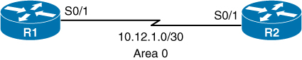
Figure 8-11 OSPF Topology with Serial Interfaces
Example 8-18 shows the relevant serial interface and OSPF configuration for R1 and R2. Notice that there are not any special commands placed in the configuration.
Example 8-18 Configuring R1 and R2 Serial and OSPF
R1
interface serial 0/1
  ip address 10.12.1.1 255.255.255.252
!
router ospf 1
   router-id 192.168.1.1
   network 0.0.0.0 255.255.255.255 area 0
R2
interface serial 0/1
  ip address 10.12.1.2 255.255.255.252
!
router ospf 1
   router-id 192.168.2.2
   network 0.0.0.0 255.255.255.255 area
Example 8-19 verifies that the OSPF network type is set to POINT_TO_POINT, indicating the OSPF point-to-point network type.
Example 8-19 Verifying the OSPF P2P Interfaces
R1# show ip ospf interface s0/1 | include Type
  Process ID 1, Router ID 192.168.1.1, Network Type POINT_TO_POINT, Cost: 64
R2# show ip ospf interface s0/1 | include Type
  Process ID 1, Router ID 192.168.2.2, Network Type POINT_TO_POINT, Cost: 64
Example 8-20 shows that point-to-point OSPF network types do not use a DR. Notice the hyphen (-) in the State field.
Example 8-20 Verifying OSPF Neighbors on P2P Interfaces
R1# show ip ospf neighbor

Neighbor ID     Pri   State           Dead Time   Address         Interface
192.168.2.2       0   FULL/  -        00:00:36    10.12.1.2      Serial0/1
Interfaces using an OSPF P2P network type form an OSPF adjacency more quickly because the DR election is bypassed, and there is no wait timer. Ethernet interfaces that are directly connected with only two OSPF speakers in the subnet could be changed to the OSPF point-to-point network type to form adjacencies more quickly and to simplify the SPF computation. The interface parameter command ip ospf network point-to-point sets an interface as an OSPF point-to-point network type.
Loopback Networks
The OSPF network type loopback is enabled by default for loopback interfaces and can be used only on loopback interfaces. The OSPF loopback network type states that the IP address is always advertised with a /32 prefix length, even if the IP address configured on the loopback interface does not have a /32 prefix length. It is possible to demonstrate this behavior by reusing Figure 8-11 and advertising a Loopback 0 interface. Example 8-21 provides the updated configuration. Notice that the network type for R2’s loopback interface is set to the OSPF point-to-point network type.
Example 8-21 OSPF Loopback Network Type
R1
interface Loopback0
    ip address 192.168.1.1 255.255.255.0
interface Serial 0/1
    ip address 10.12.1.1 255.255.255.252
!
router ospf 1
   router-id 192.168.1.1
   network 0.0.0.0 255.255.255.255 area 0
R2
interface Loopback0
    ip address 192.168.2.2 255.255.255.0
    ip ospf network point-to-point
interface Serial 0/0
    ip address 10.12.1.2 255.255.255.252
!
router ospf 1
   router-id 192.168.2.2
   network 0.0.0.0 255.255.255.255 area
The network types for the R1 and R2 loopback interfaces are checked to verify that they changed and are different, as demonstrated in Example 8-22.
Example 8-22 Displaying OSPF Network Type for Loopback Interfaces
R1# show ip ospf interface Loopback 0 | include Type
  Process ID 1, Router ID 192.168.1.1, Network Type LOOPBACK, Cost: 1
R2# show ip ospf interface Loopback 0 | include Type
Process ID 1, Router ID 192.168.2.2, Network Type POINT_TO_POINT, Cost:
Example 8-23 shows the R1 and R2 routing tables. Notice that R1’s loopback address is a /32 network, and R2’s loopback is a /24 network. Both loopbacks were configured with a /24 network; however, because R1’s Lo0 is an OSPF network type of loopback, it is advertised as a /32 network.
Example 8-23 OSPF Route Table for OSPF Loopback Network Types
R1# show ip route ospf
! Output omitted for brevity
Gateway of last resort is not set

O        192.168.2.0/24 [110/65] via 10.12.1.2, 00:02:49, Serial0/0
R2# show ip route ospf
! Output omitted for brevity
Gateway of last resort is not set
     192.168.1.0/32 is subnetted, 1 subnets
O        192.168.1.1 [110/65] via 10.12.1.1, 00:37:15, Serial0/0
Exam Preparation Tasks
As mentioned in the section “How to Use This Book” in the Introduction, you have a couple of choices for exam preparation: the exercises here, Chapter 30, “Final Preparation,” and the exam simulation questions in the Pearson Test Prep Software Online.
Review All Key Topics
Review the most important topics in the chapter, noted with the Key Topic icon in the outer margin of the page. Table 8-10 lists these key topics and the page number on which each is found.
Table 8-10 Key Topics for Chapter 8
Key Topic Element |
Description |
Page |
Paragraph |
OSPF backbone |
|
Section |
Inter-router communication |
|
OSPF Packet Types |
||
OSPF Neighbor States |
||
Paragraph |
Designated router |
|
Section |
OSPF network statement |
|
Section |
Interface specific enablement |
|
Section |
Passive interfaces |
|
Section |
Requirements for neighbor adjacency |
|
OSPF Interface Columns |
||
OSPF Neighbor State Fields |
||
Section |
Default route advertisement |
|
Section |
Link costs |
|
Section |
Failure detection |
|
Section |
Designated router elections |
|
OSPF Network Types |
Complete Tables and Lists from Memory
Print a copy of Appendix B, “Memory Tables” (found on the companion website), or at least the section for this chapter, and complete the tables and lists from memory. Appendix C, “Memory Tables Answer Key,” also on the companion website, includes completed tables and lists you can use to check your work.
Define Key Terms
Define the following key terms from this chapter and check your answers in the Glossary:
Use the Command Reference to Check Your Memory
Table 8-11 lists the important commands from this chapter. To test your memory, cover the right side of the table with a piece of paper, read the description on the left side, and see how much of the command you can remember.
Table 8-11 Command Reference
Task |
Command Syntax |
Initialize the OSPF process |
router ospf process-id |
Enable OSPF on network interfaces matching a specified network range for a specific OSPF area |
network ip-address wildcard-mask area area-id |
Enable OSPF on an explicit specific network interface for a specific OSPF area |
ip ospf process-id area area-id |
Configure a specific interface as passive |
passive interface-id |
Configure all interfaces as passive |
passive interface default |
Advertise a default route into OSPF |
default-information originate [always] [metric metric-value] [metric-type type-value] |
Modify the OSPF reference bandwidth for dynamic interface metric costing |
auto-cost reference-bandwidth bandwidth-in-mbps |
Statically set the OSPF metric for an interface |
ip ospf cost 1–65535 |
Configure the OSPF priority for a DR/BDR election |
ip ospf priority 0–255 |
Statically configure an interface as a broadcast OSPF network type |
ip ospf network broadcast |
Statically configure an interface as a point-to-point OSPF network type |
ip ospf network point-to-point |
Restart the OSPF process |
clear ip ospf process |
Display the OSPF interfaces on a router |
show ip ospf interface [brief | interface-id] |
Display the OSPF neighbors and their current states |
show ip ospf neighbor [detail] |
Display the OSPF routes that are installed in the RIB |
show ip route ospf |
References in This Chapter
RFC 2328, OSPF Version 2, by John Moy, http://www.ietf.org/rfc/rfc2328.txt, April 1998.
Edgeworth, Brad, Foss, Aaron, Garza Rios, Ramiro. IP Routing on Cisco IOS, IOS XE, and IOS XR. Indianapolis: Cisco Press: 2014.
Cisco IOS Software Configuration Guides. http://www.cisco.com.