Chapter 6
Differentiation and the Shape of Curves
IN THIS CHAPTER
![]() Locating extrema
Locating extrema
![]() Using the first and second derivative tests
Using the first and second derivative tests
![]() Interpreting concavity and points of inflection
Interpreting concavity and points of inflection
If you’ve read Chapters 4 and 5, you’re probably an expert at finding derivatives. Which is a good thing, because in this chapter you use derivatives to understand the shape of functions — where they rise, fall, max out and bottom out, how they curve, and so on.
A Calculus Road Trip
Imagine that you’re driving along the function in Figure 6-1 from left to right. Along your drive, there are several points of interest between a and l. All of them, except for the start and finish points, relate to the steepness of the road — in other words, its slope or derivative. I’m going to throw lots of new terms and definitions at you all at once here, but you shouldn’t have too much trouble because these ideas mostly involve commonsense notions like driving up or down an incline, or going over the crest of a hill.
- The function in Figure 6-1 has a derivative of zero at stationary points (level points) b, d, g, i, and k. At j, the derivative is undefined (a sharp turning point like j is a corner). These points where the derivative is either zero or undefined are the critical points of the function. The x-values of these critical points are the function’s critical numbers.
- All local maxes and mins — peaks and valleys — must occur at critical points. However, not all critical points are local maxes or mins. Point k, for instance, is a critical point but neither a max nor a min. Local maximums and minimums — or maxima and minima — are called, collectively, local extrema of the function. A single local max or min is a local extremum. Point g is the absolute maximum on the interval from a to l because it’s the highest point on the road from a to l. Point l is the absolute minimum. Note that g is also a local max, but l is not a local min because endpoints (and points of discontinuity) do not qualify as local extrema.
- The function is increasing whenever you’re going up, where the derivative is positive; it’s decreasing whenever you’re going down, where the derivative is negative. The function is also decreasing at point k, a horizontal inflection point, even though the slope and derivative are zero there. I realize that seems odd, but that’s how it works. At all horizontal inflection points, a function is either increasing or decreasing. At local extrema b, d, g, i, and j, the function is neither increasing nor decreasing.
- The function is concave up wherever it looks like a cup (rhymes with up) or a smile (or where it “holds water”) and concave down wherever it looks like a frown (rhymes with down; where it “spills water”). Wherever a function is concave up, its derivative is increasing; wherever a function is concave down, its derivative is decreasing. Inflection points c, e, h, and k are where the concavity switches from up to down or vice versa. Inflection points are also the steepest or least steep points in their immediate neighborhoods.
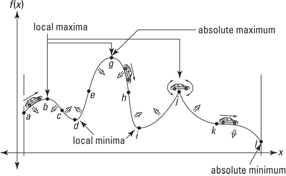
FIGURE 6-1: The graph of a function with several points of interest.
 Be careful with function sections that have a negative slope. Point c is the steepest point in its neighborhood because it has a bigger negative slope than any other nearby point. But remember, a big negative number is actually a small number, so the slope and derivative at c are actually the smallest of all the points in the neighborhood. From b to c the derivative of the function is decreasing (because it’s becoming a bigger negative). From c to d, it’s increasing (because it’s becoming a smaller negative).
Local Extrema
Now that you know what local extrema are, you need to know how to do the math to find them. Remember, all local extrema occur at critical points of a function — where the derivative is zero or undefined. So, the first step in finding a function’s local extrema is to find its critical numbers (the x-values of the critical points).
Finding the critical numbers
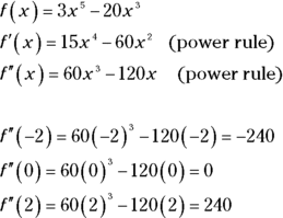
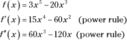
Find the critical numbers of ![]() . See Figure 6-2.
. See Figure 6-2.
- Find the first derivative of f using the power rule.
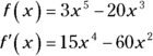
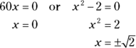
- Set the derivative equal to zero and solve for x.
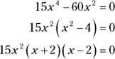
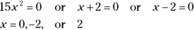

FIGURE 6-2: The graph of  .
.
These three x-values are critical numbers of f. Additional critical numbers could exist if the first derivative were undefined at some x-values, but because the derivative, ![]() , is defined for all input values, the above solution set, 0,
, is defined for all input values, the above solution set, 0, ![]() , and 2 is the complete list of critical numbers. Because the derivative of f equals zero at these three critical numbers, the curve has horizontal tangents at these numbers.
, and 2 is the complete list of critical numbers. Because the derivative of f equals zero at these three critical numbers, the curve has horizontal tangents at these numbers.
Now that you’ve got the list of critical numbers, you need to determine whether peaks or valleys or neither occur at those x-values by using either the First Derivative Test or the Second Derivative Test. (Of course, you can see where the peaks and valleys are by just looking at Figure 6-2, but you still have to learn the math.)
The First Derivative Test
The First Derivative Test is based on the Nobel-prize-caliber ideas that as you go over the top of a hill, first you go up and then you go down, and that when you drive into and out of a valley, you go down and then up. This calculus stuff is pretty amazing, isn’t it?
Take a number line and put down the critical numbers you found above: 0, ![]() , and 2. See Figure 6-3.
, and 2. See Figure 6-3.

FIGURE 6-3: The critical numbers of  .
.
This number line is now divided into four regions: to the left of ![]() , from
, from ![]() to 0, from 0 to 2, and to the right of 2. Pick a value from each region, plug it into the derivative, and note whether your result is positive or negative. Let’s use the numbers
to 0, from 0 to 2, and to the right of 2. Pick a value from each region, plug it into the derivative, and note whether your result is positive or negative. Let’s use the numbers ![]() ,
, ![]() , 1, and 3 to test the regions.
, 1, and 3 to test the regions.

These four results are, respectively, positive, negative, negative, or positive. Now, take your number line, mark each region with the appropriate positive or negative sign, and indicate whether the function is increasing (derivative is positive) or decreasing (derivative is negative). The result is a sign graph. See Figure 6-4.
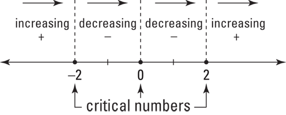
FIGURE 6-4: The sign graph for 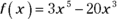 .
.
Figure 6-4 simply tells you what you already know from the graph of f — that the function goes up until ![]() , down from
, down from ![]() to 0, further down from 0 to 2, and up again from 2 on.
to 0, further down from 0 to 2, and up again from 2 on.
The function switches from increasing to decreasing at ![]() ; you go up to
; you go up to ![]() and then down. So at
and then down. So at ![]() you have a hill or a local maximum. Conversely, because the function switches from decreasing to increasing at 2, you have a valley there or a local minimum. And because the signs of the first derivative don’t switch at zero, there’s neither a min nor a max at that x-value (you get an inflection point when this happens).
you have a hill or a local maximum. Conversely, because the function switches from decreasing to increasing at 2, you have a valley there or a local minimum. And because the signs of the first derivative don’t switch at zero, there’s neither a min nor a max at that x-value (you get an inflection point when this happens).
The last step is to obtain the function values (heights) of these two local extrema by plugging the x-values into the original function:
The local max is at ![]() and the local min is at
and the local min is at ![]() .
.
The Second Derivative Test
The Second Derivative Test is based on two more prize-winning ideas: That at the crest of a hill, a road has a hump shape, so it’s curving down or concave down; and that at the bottom of a valley, a road is cup-shaped, so it’s curving up or concave up.
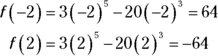
The concavity of a function at a point is given by its second derivative: A positive second derivative means the function is concave up, a negative second derivative means the function is concave down, and a second derivative of zero is inconclusive (the function could be concave up, concave down, or there could be an inflection point there). So, for our function f, all you have to do is find its second derivative and then plug in the critical numbers you found (![]() , 0, and 2) and note whether your results are positive, negative, or zero. To wit —
, 0, and 2) and note whether your results are positive, negative, or zero. To wit —
At ![]() , the second derivative is negative (
, the second derivative is negative (![]() ). This tells you that f is concave down where x equals
). This tells you that f is concave down where x equals ![]() , and therefore that there’s a local max at
, and therefore that there’s a local max at ![]() . The second derivative is positive (240) where x is 2, so f is concave up and thus there’s a local min at
. The second derivative is positive (240) where x is 2, so f is concave up and thus there’s a local min at ![]() . Because the second derivative equals zero at
. Because the second derivative equals zero at ![]() , the Second Derivative Test fails — it tells you nothing about the concavity at
, the Second Derivative Test fails — it tells you nothing about the concavity at ![]() or whether there’s a local min or max there. When this happens, you have to use the First Derivative Test.
or whether there’s a local min or max there. When this happens, you have to use the First Derivative Test.
Now go through both derivative tests one more time with another example. Find the local extrema of ![]() . See Figure 6-5.
. See Figure 6-5.

FIGURE 6-5: The graph of  .
.
- Find the first derivative of g.
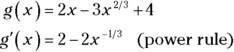
- Set the derivative equal to zero and solve.
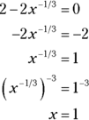
Thus 1 is a critical number.
-
Determine whether the first derivative is undefined for any x-values.
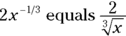 Now, because the cube root of zero is zero, if you plug in zero to
  , you’d have
  , which is undefined. So the derivative,
  is undefined at
  , and thus 0 is another critical number.
 -
Plot the critical numbers on a number line, and then use the First Derivative Test to figure out the sign of each region.
You can use
 , 0.5, and 2 as test numbers
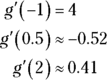
Figure 6-6 shows the sign graph.
Because the first derivative of g switches from positive to negative at 0, there’s a local max there. And because the first derivative switches from negative to positive at 1, there’s a local min at
 .
. - Plug the critical numbers into g to obtain the function values (the heights) of these two local extrema.
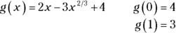

FIGURE 6-6: The sign graph of  .
.
So, there’s a local max at (0, 4) and a local min at (1, 3).
You could have used the Second Derivative Test instead of the First in Step 4. You’d need the second derivative of g, which is, as you know, the derivative of its first derivative:
Evaluate the second derivative at 1 (the critical number where ![]() ).
).
Because ![]() is positive, you know that g is concave up at
is positive, you know that g is concave up at ![]() and, therefore, that there’s a local min there. The Second Derivative Test is no help where the first derivative is undefined (where
and, therefore, that there’s a local min there. The Second Derivative Test is no help where the first derivative is undefined (where ![]() ), so you’ve got to use the First Derivative Test for that critical number.
), so you’ve got to use the First Derivative Test for that critical number.
Finding Absolute Extrema on a Closed Interval
Every function that’s continuous on a closed interval has an absolute maximum and an absolute minimum value in that interval — a highest and lowest point — though, as you see in the following example, there can be a tie for highest or lowest value.
 A closed interval like [2, 5] includes the endpoints 2 and 5. An open interval like (2, 5) excludes the endpoints.
Finding the absolute max and min is a snap. All you do is compute the critical numbers of the function in the given interval, determine the height of the function at each critical number, and then figure the height of the function at the two endpoints of the interval. The greatest of this set of heights is the absolute max; and the least is the absolute min. Example: Find the absolute max and min of ![]() in the closed interval
in the closed interval ![]() .
.
- Find the critical numbers of h in the open interval
 .
.
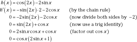

Thus, the zeros of
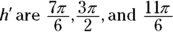 , and because
  is defined for all input numbers, this is the complete list of critical numbers.
 - Compute the function values (the heights) at each critical number.
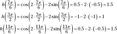
- Determine the function values at the endpoints of the interval.
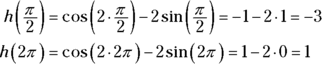
So, from Steps 2 and 3, you’ve found five heights: 1.5, 1, 1.5,
 , and 1. The largest number in this list, 1.5, is the absolute max; the smallest,
  , is the absolute min.
The absolute max occurs at two points: ![]() and
and ![]() . The absolute min occurs at one of the endpoints,
. The absolute min occurs at one of the endpoints, ![]() . Figure 6-7 shows the graph of h.
. Figure 6-7 shows the graph of h.

FIGURE 6-7: The graph of 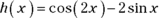 .
.
Finding Absolute Extrema over a Function’s Entire Domain
A function’s absolute max and absolute min over its entire domain are the highest and lowest values of the function anywhere it’s defined. A function can have an absolute max or min or both or neither. For example, the parabola ![]() has an absolute min at the point (0, 0) — the bottom of its cup shape — but no absolute max because it goes up forever to the left and the right. You could say that its absolute max is infinity if it weren’t for the fact that infinity is not a number and thus it doesn’t qualify as a maximum (ditto, of course, for negative infinity as a minimum).
has an absolute min at the point (0, 0) — the bottom of its cup shape — but no absolute max because it goes up forever to the left and the right. You could say that its absolute max is infinity if it weren’t for the fact that infinity is not a number and thus it doesn’t qualify as a maximum (ditto, of course, for negative infinity as a minimum).
The basic idea is this: Either a function will max out somewhere or it will go up forever to infinity. And the same idea applies to a min and going down to negative infinity.
To locate a function’s absolute max and min over its domain, find the height of the function at each of its critical numbers — just like in the previous section, except that here you consider all the critical numbers, not just those in a given interval. The highest of these values is the absolute max unless the function rises to positive infinity somewhere, in which case you say that it has no absolute max. The lowest of these values is the absolute min, unless the function goes down to negative infinity, in which case it has no absolute min.
If a function goes up or down infinitely, it does so at its extreme right or left or at a vertical asymptote. So, your last step (after evaluating all the critical points) is to evaluate ![]() and
and ![]() — the so-called end behavior of the function — and the limit of the function as x approaches each vertical asymptote from the left and from the right. If any of these limits equals positive infinity, then the function has no absolute max; if none equals positive infinity, then the absolute max is the function value at the highest of the critical points. And if any of these limits is negative infinity, then the function has no absolute min; if none of them equals negative infinity, then the absolute min is the function value at the lowest of the critical points.
— the so-called end behavior of the function — and the limit of the function as x approaches each vertical asymptote from the left and from the right. If any of these limits equals positive infinity, then the function has no absolute max; if none equals positive infinity, then the absolute max is the function value at the highest of the critical points. And if any of these limits is negative infinity, then the function has no absolute min; if none of them equals negative infinity, then the absolute min is the function value at the lowest of the critical points.
Figure 6-8 shows a couple functions where the above method won’t work. The function ![]() has no absolute max despite the fact that it doesn’t go up to infinity. Its max isn’t 4 because it never gets to 4, and its max can’t be anything less than 4, like 3.999, because it gets higher than that, say 3.9999. The function
has no absolute max despite the fact that it doesn’t go up to infinity. Its max isn’t 4 because it never gets to 4, and its max can’t be anything less than 4, like 3.999, because it gets higher than that, say 3.9999. The function ![]() has no absolute min despite the fact that it doesn’t go down to negative infinity. Going left,
has no absolute min despite the fact that it doesn’t go down to negative infinity. Going left, ![]() crawls along the horizontal asymptote at
crawls along the horizontal asymptote at ![]() . g gets lower and lower, but it never gets as low as zero, so neither zero nor any other number can be the absolute min.
. g gets lower and lower, but it never gets as low as zero, so neither zero nor any other number can be the absolute min.

FIGURE 6-8: Two functions with no absolute extrema.
Concavity and Inflection Points
Look back at the function ![]() in Figure 6-2. You used the three critical numbers of f,
in Figure 6-2. You used the three critical numbers of f, ![]() 0, and 2, to find the function’s local extrema:
0, and 2, to find the function’s local extrema: ![]() and
and ![]() . This section investigates what happens elsewhere on this function — specifically, where the function is concave up or down and where the concavity switches (the inflection points).
. This section investigates what happens elsewhere on this function — specifically, where the function is concave up or down and where the concavity switches (the inflection points).
The process for finding concavity and inflection points is analogous to using the First Derivative Test and the sign graph to find local extrema, except that now you use the second derivative.
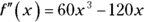
- Find the second derivative of f.
- Set the second derivative equal to zero and solve.
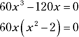
-
Determine whether the second derivative is undefined for any x-values.
 is defined for all real numbers, so there are no other x-values to add to the list from Step 2.
Steps 2 and 3 give you what you could call second derivative critical numbers of f because they are analogous to the critical numbers of f that you find using the first derivative. But, as far as I’m aware, this set of numbers has no special name. In any event, the important thing to know is that this list is made up of the zeros of
 plus any x-values where
  is undefined.
 -
Plot these numbers on a number line and test the regions with the second derivative.
Use
 1, and 2 as test numbers (Figure 6-9 shows the sign graph).
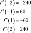
A positive sign on this sign graph tells you that the function is concave up in that interval; negative means concave down. The function has an inflection point (usually) at any x-value where the signs switch from positive to negative or vice versa.
Because the signs switch at
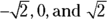 and because these three numbers are zeros of
  , inflection points occur at these x-values. But in a problem where the signs switch at a number where
  is undefined, you have to check one more thing before you can conclude that there’s an inflection point there. An inflection point exists at a given x-value only if there’s a tangent line to the function at that number. This is the case wherever the first derivative exists or where there’s a vertical tangent.
 - Plug these three x-values into f to obtain the function values of the three inflection points.

The square root of two equals about 1.4, so there are inflection points at about
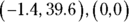 , and about
  .
.

FIGURE 6-9: A second derivative sign graph for  .
.
Graphs of Derivatives
You can learn a lot about functions and their derivatives by comparing the important features of their graphs. Let’s keep going with the same function ![]() ; travel along f from left to right (see Figure 6-10), pausing to observe its points of interest and what’s happening to the graph of
; travel along f from left to right (see Figure 6-10), pausing to observe its points of interest and what’s happening to the graph of ![]() at the same points. But first a (long) warning:
at the same points. But first a (long) warning:

FIGURE 6-10:  and its first derivative,
  .
.
Looking at the graph of ![]() in Figure 6-10, or the graph of any derivative, you may need to remind yourself frequently that “This is the derivative I’m looking at, not the function!” You’ve looked at so many graphs of functions over the years that when you start looking at graphs of derivatives, you can easily lapse into thinking of them as regular functions. You might, for instance, look at an interval that’s going up on the graph of a derivative and mistakenly conclude that the original function must also be going up in the same interval — an easy mistake to make. You know that the first derivative is the same thing as slope. So, when you see the graph of the first derivative going up, you may think, “Oh, the first derivative (the slope) is going up, and when the slope goes up that’s like going up a hill, so the original function must be rising.” This sounds reasonable because, loosely speaking, you can describe the front side of a hill as a slope that’s going up, increasing. But mathematically speaking, the front side of a hill has a positive slope, not necessarily an increasing slope. So, where a function is increasing, the graph of its derivative will be positive, but the derivative might be going up or down. Say you’re going up a hill. As you approach the top, you’re still going up, but the slope (the steepness) is going down. It might be 3, then 2, then 1, and then at the top the slope is zero. In such an interval, the graph of the function is increasing, but the graph of its derivative is decreasing. Got that?
in Figure 6-10, or the graph of any derivative, you may need to remind yourself frequently that “This is the derivative I’m looking at, not the function!” You’ve looked at so many graphs of functions over the years that when you start looking at graphs of derivatives, you can easily lapse into thinking of them as regular functions. You might, for instance, look at an interval that’s going up on the graph of a derivative and mistakenly conclude that the original function must also be going up in the same interval — an easy mistake to make. You know that the first derivative is the same thing as slope. So, when you see the graph of the first derivative going up, you may think, “Oh, the first derivative (the slope) is going up, and when the slope goes up that’s like going up a hill, so the original function must be rising.” This sounds reasonable because, loosely speaking, you can describe the front side of a hill as a slope that’s going up, increasing. But mathematically speaking, the front side of a hill has a positive slope, not necessarily an increasing slope. So, where a function is increasing, the graph of its derivative will be positive, but the derivative might be going up or down. Say you’re going up a hill. As you approach the top, you’re still going up, but the slope (the steepness) is going down. It might be 3, then 2, then 1, and then at the top the slope is zero. In such an interval, the graph of the function is increasing, but the graph of its derivative is decreasing. Got that?
Okay, let’s get back to f and its derivative, shown in Figure 6-10. Remember, before the warning we were traveling along f from left to right. Beginning on the left, f increases until the local max at ![]() . It’s going up, so its slope is positive, but f is getting less steep so its slope is decreasing — the slope decreases until it becomes zero at the peak. This corresponds to the graph of
. It’s going up, so its slope is positive, but f is getting less steep so its slope is decreasing — the slope decreases until it becomes zero at the peak. This corresponds to the graph of ![]() (the slope) which is positive (because it’s above the x-axis) but decreasing as it goes down to the point
(the slope) which is positive (because it’s above the x-axis) but decreasing as it goes down to the point ![]() .
.
 Ready for some rules about how the graph of a function compares to the graph of its derivative? Well, ready or not, here you go:
- An increasing interval on a function corresponds to an interval on the graph of its derivative that’s positive (or zero for one point if the function has a horizontal inflection point). In other words, a function’s increasing interval corresponds to a part of the derivative graph that’s above the x-axis (or that touches the axis for a single point in the case of a horizontal inflection point). See intervals A and F in Figure 6-10.
-
A local max on the graph of a function corresponds to a zero (or x-intercept) on an interval of the graph of its derivative that crosses the x-axis going down.
 When you look at points on a derivative graph, don’t forget that the y-coordinate of a point — like
  — on a graph of a first derivative tells you the slope of the original function, not its height. Think of the y-axis on a first derivative graph as the slope-axis or the m-axis.
 - A decreasing interval on a function corresponds to a negative interval on the graph of the derivative (or zero for one point if the function has a horizontal inflection point). The negative interval on the derivative graph is below the x-axis (or in the case of a horizontal inflection point, the derivative graph touches the x-axis at a single point). See intervals B, C, D, and E in Figure 6-10, where f goes down all the way to the local min at
 and where
  is negative — except for the point (0, 0) — until it gets to (2, 0).
 - A local min on the graph of a function corresponds to a zero (or x-intercept) on an interval of the graph of its derivative that crosses the x-axis going up.
Now retrace your steps and look at the concavity and inflection points of f in Figure 6-10. First, consider intervals A and B in the figure. Starting from the left again, the graph of f is concave down — a decreasing slope — until it gets to the inflection point at about ![]() . So, the graph of
. So, the graph of ![]() decreases until it bottoms out at about
decreases until it bottoms out at about ![]() . These coordinates tell you that the inflection point at
. These coordinates tell you that the inflection point at ![]() on f has a slope of
on f has a slope of ![]() . Note that the inflection point at
. Note that the inflection point at ![]() is the steepest point on that stretch of the function, but it has the smallest slope because its slope is a larger negative than the slope at any nearby point.
is the steepest point on that stretch of the function, but it has the smallest slope because its slope is a larger negative than the slope at any nearby point.
Between ![]() and the next inflection point at (0, 0), f is concave up, which means the same thing as an increasing slope. So the graph of
and the next inflection point at (0, 0), f is concave up, which means the same thing as an increasing slope. So the graph of ![]() increases from about
increases from about ![]() to where it hits a local max at (0, 0). See interval C in Figure 6-10.
to where it hits a local max at (0, 0). See interval C in Figure 6-10.
Time for a couple more rules:
- A concave down interval on the graph of a function corresponds to a decreasing interval on the graph of its derivative — intervals A, B, and D in Figure 6-10. And a concave up interval on the function corresponds to an increasing interval on the derivative — intervals C, E, and F.
- An inflection point on a function (except for a vertical inflection point where the derivative is undefined) corresponds to a local extremum on the graph of its derivative. An inflection point of minimum slope corresponds to a local min on the derivative graph; an inflection point of maximum slope corresponds to a local max on the derivative graph.
After (0, 0), f is concave down till the inflection point at about ![]() — this corresponds to the decreasing section of
— this corresponds to the decreasing section of ![]() from (0, 0) to its min at
from (0, 0) to its min at ![]() — interval D in Figure 6-10. Finally, f is concave up the rest of the way, which corresponds to the increasing section of
— interval D in Figure 6-10. Finally, f is concave up the rest of the way, which corresponds to the increasing section of ![]() beginning at
beginning at ![]() — intervals E and F in Figure 6-10.
— intervals E and F in Figure 6-10.
The Mean Value Theorem
You don’t need the Mean Value Theorem for much, but it’s a famous and important theorem, so you really should learn it. Look at Figure 6-11 and see if you can make sense of the mumbo jumbo beneath it.
![Graph depicting the mean value theorem, where f is continuous on the closed interval [a, b] and differentiable on the open interval (a, b).](http://images-20200215.ebookreading.net/2/5/5/9781119591207/9781119591207__calculus-essentials-for__9781119591207__images__9781119591207-fg0611.png)
FIGURE 6-11: An illustration of the Mean Value Theorem.
 The Mean Value Theorem: If f is continuous on the closed interval [a, b] and differentiable on the open interval (a, b), then there exists at least one number c in (a, b) such that
Okay, so here’s what the theorem means. The secant line connecting points ![]() and
and ![]() in Figure 6-11 has a slope given by the slope formula:
in Figure 6-11 has a slope given by the slope formula:
Note that this is the same as the right side of the equation in the mean value theorem. The derivative at a point is the same thing as the slope of the tangent line at that point, so the theorem just says that there must be at least one point between a and b where the slope of the tangent is the same as the slope of the secant line from a to b. The result is parallel lines like you see in Figure 6-11.