IN THIS CHAPTER

Discovering the simple algebra behind the calculus

Finding the derivatives of lines and curves

Tackling the tangent line problem and the difference quotient

Differential calculus is the mathematics of change and of infinitesimals. You might say it’s the mathematics of infinitesimal changes — changes that occur every gazillionth of a second.

Without differential calculus — if you’ve got only algebra, geometry, and trigonometry — you’re limited to the mathematics of things that either don’t change or that change or move at an unchanging rate. Remember those problems from algebra? One train leaves the station at 3 p.m. going west at 80 mph. Two hours later another train leaves going east at 50 mph… . You can handle such a problem with algebra because the speeds or rates are unchanging. Our world, however, isn’t one of unchanging rates — rates are in constant flux.

Think about putting men on the moon. Apollo 11 took off from a moving launch pad (the earth is both rotating on its axis and revolving around the sun). As the Apollo flew higher and higher, the friction caused by the atmosphere and the effect of the earth’s gravity were changing not just every second, not just every millionth of a second, but every infinitesimal fraction of a second. The spacecraft’s weight was also constantly changing as it burned fuel. All of these things influenced the rocket’s changing speed. On top of all that, the rocket had to hit a moving target, the moon. All of these things were changing, and their rates of change were changing. Say the rocket was going 1000 mph one second and 1020 mph a second later — during that one second, the rocket’s speed literally passed through the infinite number of different speeds between 1000 and 1020 mph. How can you do the math for these ephemeral things that change every infinitesimal part of a second? You can’t do it without differentiation.

Differential calculus is used for all sorts of terrestrial things as well. Modern economic theory, for example, relies on differentiation. In economics, everything is in constant flux. Prices go up and down, supply and demand fluctuate, and inflation is constantly changing. These things are constantly changing, and the ways they affect each other are constantly changing. You need calculus for this.

The Derivative: It’s Just Slope

Differentiation is the first of the two major ideas in calculus (the other is integration). Differentiation is the process of finding the derivative of a function like . The derivative is just a fancy calculus term for a simple idea you know from algebra: slope. Slope, as you know, is the fancy algebra term for steepness.

In differential calculus, you study differentiation, which is the process of deriving — that’s finding — derivatives. These are big words for a simple idea: finding the steepness or slope of a line or curve. Throw some of these terms around to impress your friends.

Consider Figure 4-1. A steepness of 1/2 means that as the stickman walks one foot to the right, he goes up 1/2 foot; where the steepness is 3, he goes up 3 feet as he walks 1 foot to the right. Where the steepness is zero, he’s at the top, going neither up nor down; and where the steepness is negative, he’s going down. A steepness of , for example, means that he goes down 2 feet for every foot he goes to the right.

The slope of a line

By now you should know that slope is what differentiation is all about. Consider the line . Plug 1 into x and y equals 5, which gives you the point located at (1, 5); plug 2 into x and y equals 7, giving you the point (2, 7); plug 3 into x and y equals 9, that’s the point (3, 9), and so on. Now let’s calculate the line’s slope (yes, I realize that tells me that the slope is 2; just humor me). Recall that

The rise is the vertical distance between two points, and the run is the horizontal distance between the two points. Now, take any two points on the line, say, (1, 5) and (6, 15), and figure the rise and the run. You rise up 10 from (1, 5) to (6, 15) because 5 plus 10 is 15. And you run across 5 from (1, 5) to (6, 15) because 1 plus 5 is 6. Next, divide to get the slope:

Here’s how you do the same problem using the slope formula:

Plug in the points (1, 5) and (6, 15):

The Derivative: It’s Just a Rate

Here’s another way to understand the idea of a derivative that’s even more fundamental than the concept of slope: A derivative is a rate. So why did I start the chapter with slope? Because slope is in some respects the easier of the two concepts, and slope is the idea you return to again and again in this book and any other calculus textbook as you look at the graphs of dozens of functions. But before you’ve got a slope, you’ve got a rate. A slope is, in a sense, a picture of a rate; the rate comes first, the picture of it comes second. Just like you can have a function before you see its graph, you can have a rate before you see it as a slope.

Calculus on the playground

Imagine Laurel and Hardy on a teeter-totter — see Figure 4-2.

Assuming Hardy weighs twice as much as Laurel, Hardy has to sit twice as close to the center as Laurel for them to balance. And for every inch that Hardy goes down, Laurel goes up two. So Laurel moves twice as much as Hardy. Voilà, you’ve got a derivative!

A derivative is simply a measure of how much one thing changes compared to another — and that’s a rate.

Laurel moves twice as much as Hardy, so you write

Loosely speaking, dL can be thought of as the change in Laurel’s position, and dH as the change in Hardy’s position. You can see that if Hardy goes down 10 inches, then dH is 10, and because dL equals 2 times dH, dL is 20 — so Laurel goes up 20 inches. Dividing both sides of this equation by dH gives you

And that’s the derivative of Laurel with respect to Hardy. (It’s read as, “dee L, dee H,” or as, “the derivative of L with respect to H.”) The fact that simply means Laurel is moving 2 times as much as Hardy. Laurel’s rate of movement is 2 inches per inch of Hardy’s movement.

Now let’s look at it from Hardy’s point of view. Hardy moves half as much as Laurel, so you can also write

Dividing by dL gives you

This is the derivative of Hardy with respect to Laurel, and it means Hardy moves inch for every inch Laurel moves. Thus, Hardy’s rate is inch per inch of Laurel’s movement. By the way, you can also get this derivative by taking , which is the same as , and flipping it upside down to get .

These rates of 2 inches per inch and inch per inch may seem odd because we often think of rates as referring to something per unit of time, like miles per hour. But a rate can be anything per anything. So, whenever you’ve got a this per that, you’ve got a rate; and if you’ve got a rate, you’ve got a derivative.

There’s no end to the different rates you might see: miles per gallon (for gas mileage), gallons per minute (for water draining out of a pool), output per employee (for a factory’s productivity), and so on. Rates can be constant or changing. In either case, every rate is a derivative, and every derivative is a rate.

The rate-slope connection

Rates and slopes have a simple connection. The previous rate examples can be graphed on an x-y coordinate system, where each rate appears as a slope. Laurel moving twice as much as Hardy can be represented by the following equation:

Figure 4-3 shows the graph of this function.

The inches on the H-axis indicate how far Hardy has moved up or down from the teeter-totter’s starting position; the inches on the L-axis show how far Laurel has moved up or down. The line goes up 2 inches for each inch it goes to the right, and its slope is thus , or 2. This is the visual depiction of , and it shows that Laurel’s position changes 2 times as much as Hardy’s.

One last comment. You know that . Well, you can think of dL as the rise and dH as the run. That ties everything together.

Don’t forget, a derivative is a slope, and a derivative is a rate.

The Derivative of a Curve

The previous sections in this chapter involve linear functions — straight lines with unchanging slopes. But if all functions and graphs were lines with unchanging slopes, there’d be no need for calculus. The derivative of the Laurel and Hardy function graphed previously is 2, but you don’t need calculus to determine the slope of a line. Calculus is the mathematics of change, so now is a good time to move on to parabolas, curves with changing slopes. Figure 4-4 is the graph of the parabola, .

Notice how the parabola gets steeper and steeper as you go to the right. You can see from the graph that at the point (2, 1), the slope is 1; at (4, 4), the slope is 2; at (6, 9), the slope is 3, and so on. It turns out that the derivative of this function equals (I show you how I got that in a minute). To find the slope of the curve at any point, you just plug the x-coordinate of the point into the derivative, , and you’ve got the slope. For instance, if you want the slope at the point (3, 2.25), plug 3 into the x, and the slope is times 3, or 1.5.

Here’s the calculus. You write

And you say,

The derivative of the function .

I promised to tell you how to derive this derivative of :

1. Take the power and put it in front of the coefficient.

   

2. Multiply.
   

3. Reduce the power by 1.

   In this example the 2 becomes a 1. So the derivative is

   

The Difference Quotient

Sound the trumpets! You come now to what is perhaps the cornerstone of differential calculus: the difference quotient, the bridge between limits and the derivative. (But you’re going to have to be patient here, because it’s going to take me a few pages to explain the logic behind the difference quotient before I can show you what it is.) Okay, so here goes. You know that a derivative is just a slope. You know all about the slope of a line, and in Figure 4-4, I gave you the slope of the parabola at several points and showed you the short-cut for finding the derivative — but I left out the important math in the middle. That math involves limits and the difference quotient, and takes us to the threshold of calculus. Hold on to your hat.

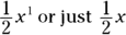
To compute a slope, you need two points to plug into the slope formula. For a line, this is easy. You just pick any two points on the line and plug them in. But say you want the slope of the parabola in Figure 4-5 at the point (2, 4).

You can see the line drawn tangent to the curve at (2, 4), and because the slope of the tangent line is the same as the slope of the parabola at (2, 4), all you need is the slope of the tangent line. But you don’t know the equation of the tangent line, so you can’t get the second point — in addition to (2, 4) — that you need for the slope formula. Here’s how the inventors of calculus got around this roadblock. Figure 4-5 also shows a secant line (a line intersecting a curve at two points) intersecting the parabola at (2, 4) and at (10, 100).

The slope of this secant line is given by the slope formula:

This secant line is quite a bit steeper than the tangent line, so the slope of the secant, 12, is higher than the slope you’re looking for.

Now add one more point at (6, 36) and draw another secant using that point and (2, 4) again. See Figure 4-6.

Calculate the slope of this second secant:

You can see that this secant line is a better approximation of the tangent line than the first secant. Now, imagine what would happen if you grabbed the point at (6, 36) and slid it down the parabola toward (2, 4), dragging the secant line along with it. Can you see that as the point gets closer and closer to (2, 4), the secant line gets closer and closer to the tangent line, and that the slope of this secant thus gets closer and closer to the slope of the tangent?

So, you can get the slope of the tangent if you take the limit of the slope of this moving secant. Let’s give the moving point the coordinates . As this point slides closer and closer to , namely (2, 4), the run — that’s — gets closer and closer to zero. So here’s the limit you need:

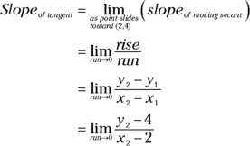
Watch what happens to this limit when you plug in three more points on the parabola that are closer and closer to (2, 4):

• When the point slides to (2.1, 4.41), the slope is 4.1. When the point slides to (2.01, 4.0401), the slope is 4.01. When the point slides to (2.001, 4.004001), the slope is 4.001.

Sure looks like the slope is headed toward 4.

As with all limit problems, the variable in this problem, the run, approaches but never actually gets to zero. If it got to zero — which would happen if you slid the point you grabbed along the parabola until it was actually on top of (2, 4) — you’d have a slope of , which is undefined. But, of course, that’s precisely the slope you want — the slope of the line when the point does land on top of (2, 4). Herein lies the beauty of the limit process. With this limit, you get the exact slope of the tangent line even though the limit function,, generates slopes of secant lines.

Here again is the equation for the slope of the tangent line:

And the slope of the tangent line is — yes — the derivative.

The derivative of a function at some number , written , is the slope of the tangent line to f drawn at c.

The slope fraction is expressed with algebra terminology. Now let’s rewrite it to give it that highfalutin calculus look. But first, finally, the definition you’ve been waiting for:

Definition of the Difference Quotient: There’s a calculus term for the general slope fraction, or , when you write it in the fancy calculus way. A fraction is a quotient, right? And both and are differences, right? So, voilà, it’s called the difference quotient. Here it is:

In the next two pages I show you how morphs into the difference quotient.

Okay, let’s lay out this morphing process. First, the run, (in this example, ), is called — don’t ask me why — h. Next, because and the run equals h, equals . You then write as and as . Making all the substitutions gives you the derivative of at :

is simply the shrinking stair step you can see in Figure 4-6 as the point slides down the parabola toward (2, 4).

Figure 4-7 is like Figure 4-6 except that instead of exact points like (6, 36) and (10, 100), the sliding point has the general coordinates of and the rise and the run are expressed in terms of h.

Doing the math gives you the slope of the tangent line at (2, 4):

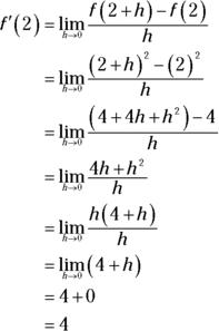
So the slope is 4. (By the way, it’s just a coincidence that the slope at (2, 4) happens to be the same as the y-coordinate of the point.)

Definition of the Derivative: If you replace the point in the above limit equation with the general point , you get the general definition of the derivative as a function of x:

So at last you see that the derivative is defined as the limit of the difference quotient.

Now work out this limit and get the derivative for the parabola .

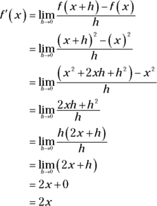
Thus for this parabola, the derivative — that’s the slope of the tangent line — equals 2x. Plug any number into x, and you get the slope of the parabola at that x-value! Try it.

Average and Instantaneous Rate

Returning once again to the connection between slopes and rates, a slope is just the visual depiction of a rate: The slope, , just tells you the rate at which y changes compared to x. If, for example, y is the number of miles and x is the number of hours, you get the familiar rate of miles per hour.

Each secant line in Figure 4-6 has a slope given by the formula . That slope is the average rate over the interval from . If y is in miles and x is in hours, you get the average speed in miles per hour during the time interval from .

When you take the limit and get the slope of the tangent line, you get the instantaneous rate at the point . Again, if y is in miles and x is in hours, you get the instantaneous speed at the point in time, . Because the slope of the tangent line is the derivative, this gives us another definition of the derivative.

The derivative of a function at some x-value is the instantaneous rate of change of f with respect to x at that value.

Three Cases Where the Derivative Does Not Exist

By now you certainly know that the derivative of a function at a given point is the slope of the tangent line at that point. So, if you can’t draw a tangent line, there’s no derivative — that happens in two cases. In the third case, there’s a tangent line, but its slope and the derivative are undefined:

1. There’s no tangent line and thus no derivative at any type of discontinuity: infinite, removable, or jump. Continuity is, therefore, a necessary condition for differentiability. It’s not, however, a sufficient condition as the next two cases show. Dig that logician-speak.
2. There’s no tangent line and thus no derivative at a sharp corner on a function (or at a cusp, a really pointy, sharp turn). See function f in Figure 4-8.
3. Where a function has a vertical inflection point (see function g), the slope is undefined and thus the derivative fails to exist.