Chapter 1
Calculus: No Big Deal
IN THIS CHAPTER
![]() Calculus — it’s just souped-up regular math
Calculus — it’s just souped-up regular math
![]() Zooming in is the key
Zooming in is the key
![]() Delving into the derivative: It’s a rate or a slope
Delving into the derivative: It’s a rate or a slope
![]() Investigating the integral — addition for experts
Investigating the integral — addition for experts
In this chapter, I answer the question “What is calculus?” in plain English and give you real-world examples of how it’s used. Then I introduce you to the two big ideas in calculus: differentiation and integration. Finally, I explain why calculus works. After reading this chapter, you will understand what calculus is all about.
So What Is Calculus Already?
Calculus is basically just very advanced algebra and geometry. In one sense, it’s not even a new subject — it takes the ordinary rules of algebra and geometry and tweaks them so that they can be used on more complicated problems. (The rub, of course, is that darn other sense in which it is a new and more difficult subject.)
Look at Figure 1-1. On the left is a man pushing a crate up a straight incline. On the right, the man is pushing the same crate up a curving incline. The problem, in both cases, is to determine the amount of energy required to push the crate to the top. You can do the problem on the left with regular math. For the one on the right, you need calculus (if you don’t know the physics shortcuts).

FIGURE 1-1: The difference between regular math and calculus: In a word, it’s the curve.
For the straight incline, the man pushes with an unchanging force, and the crate goes up the incline at an unchanging speed. With some simple physics formulas and regular math (including algebra and trig), you can compute how many calories of energy are required to push the crate up the incline. Note that the amount of energy expended each second remains the same.
For the curving incline, on the other hand, things are constantly changing. The steepness of the incline is changing — and it’s not like it’s one steepness for the first 3 feet and then a different steepness for the next 3 — it’s constantly changing. And the man pushes with a constantly changing force — the steeper the incline, the harder the push. As a result, the amount of energy expended is also changing, not just every second or thousandth of a second, but constantly, from one moment to the next. That’s what makes it a calculus problem. It should come as no surprise to you, then, that calculus is called “the mathematics of change.” Calculus takes the regular rules of math and applies them to fluid, evolving problems.
For the curving incline problem, the physics formulas remain the same, and the algebra and trig you use stay the same. The difference is that — in contrast to the straight incline problem, which you can sort of do in a single shot — you’ve got to break up the curving incline problem into small chunks and do each chunk separately. Figure 1-2 shows a small portion of the curving incline blown up to several times its size.

FIGURE 1-2: Zooming in on the curve — voilà, it’s straight (almost).
When you zoom in far enough, the small length of the curving incline becomes practically straight. Then you can solve that small chunk just like the straight incline problem. Each small chunk can be solved the same way, and then you just add up all the chunks.
That’s calculus in a nutshell. It takes a problem that can’t be done with regular math because things are constantly changing — the changing quantities show up on a graph as curves — it zooms in on the curve till it becomes straight, and then it finishes off the problem with regular math.
What makes calculus such a fantastic achievement is that it does what seems impossible: it zooms in infinitely. As a matter of fact, everything in calculus involves infinity in one way or another, because if something is constantly changing, it’s changing infinitely often from each infinitesimal moment to the next.
Real-World Examples of Calculus
So, with regular math you can do the straight incline problem; with calculus you can do the curving incline problem. With regular math you can determine the length of a buried cable that runs diagonally from one corner of a park to the other (remember the Pythagorean Theorem?). With calculus you can determine the length of a cable hung between two towers that has the shape of a catenary (which is different, by the way, from a simple circular arc or a parabola). Knowing the exact length is of obvious importance to a power company planning hundreds of miles of new electric cable.
You can calculate the area of the flat roof of a home with regular math. With calculus you can compute the area of a complicated, nonspherical shape like the dome of the Minneapolis Metrodome. Architects need to know the dome’s area to determine the cost of materials and to figure the weight of the dome (with and without snow on it). The weight, of course, is needed for planning the strength of the supporting structure.
With regular math and simple physics, you can calculate how much a quarterback must lead a pass receiver if the receiver runs in a straight line and at a constant speed. But when NASA, in 1975, calculated the necessary “lead” for aiming the Viking I at Mars, it needed calculus because both the Earth and Mars travel on elliptical orbits, and the speeds of both are constantly changing — not to mention the fact that on its way to Mars, the spacecraft was affected by the different and constantly changing gravitational pulls of the Earth, moon, Mars, the sun. See Figure 1-3.

FIGURE 1-3: B.C.E. (Before the Calculus Era) and C.E. (the Calculus Era).
Differentiation
Differentiation is the first big idea in calculus. It’s the process of finding a derivative of a curve. And a derivative is just the fancy calculus term for a curve’s slope or steepness.
In algebra, you learned the slope of a line is equal to the ratio of the rise to the run. In other words, ![]() . In Figure 1-4, the rise is half as long as the run, so segment AB has a slope of 1/2. On a curve, the slope is constantly changing, so you need calculus to determine its slope.
. In Figure 1-4, the rise is half as long as the run, so segment AB has a slope of 1/2. On a curve, the slope is constantly changing, so you need calculus to determine its slope.

FIGURE 1-4: Calculating the slope of a curve isn’t as simple as rise over run.
The slope of segment AB is the same at every point from A to B. But the steepness of the curve is changing between A and B. At A, the curve is less steep than the segment, and at B the curve is steeper than the segment. So what do you do if you want the exact slope at, say, point C? You just zoom in. See Figure 1-5.

FIGURE 1-5: Zooming in on the curve.
When you zoom in far enough — actually infinitely far — the little piece of the curve becomes straight, and you can figure the slope the old-fashioned way. That’s how differentiation works.
Integration
Integration, the second big idea in calculus, is basically just fancy addition. Integration is the process of cutting up an area into tiny sections, figuring out their areas, and then adding them up to get the whole area. Figure 1-6 shows two area problems — one that you can do with geometry and one where you need calculus.

FIGURE 1-6: If you can’t determine the area on the left, hang up your calculator.
The shaded area on the left is a simple rectangle, so its area, of course, equals length times width. But you can’t figure the area on the right with regular geometry because there’s no area formula for this funny shape. So what do you do? Why, zoom in, of course. Figure 1-7 shows the top portion of a narrow strip of the weird shape blown up to several times its size.

FIGURE 1-7: For the umpteenth time: When you zoom in, curves become straight.
When you zoom in, the curve becomes practically straight, and the further you zoom in, the straighter it gets — with integration, you actually zoom in infinitely close, sort of. You end up with the shape on the right in Figure 1-7, an ordinary trapezoid — or a triangle sitting on top of a rectangle. Because you can compute the areas of rectangles, triangles, and trapezoids with ordinary geometry, you can get the area of this and all the other thin strips and then add up all these areas to get the total area. That’s integration.
Why Calculus Works
The mathematics of calculus works because curves are locally straight; in other words, they’re straight at the microscopic level. The earth is round, but to us it looks flat because we’re sort of at the microscopic level when compared to the size of the earth. Calculus works because when you zoom in and curves become straight, you can use regular algebra and geometry with them. This zooming-in process is achieved through the mathematics of limits.
Limits: Math microscopes
The mathematics of limits is the microscope that zooms in on a curve. Say you want the exact slope or steepness of the parabola ![]() at the point (1, 1). See Figure 1-8.
at the point (1, 1). See Figure 1-8.

FIGURE 1-8: The parabola  with a tangent line at (1, 1).
With the slope formula from algebra, you can figure the slope of the line between (1, 1) and (2, 4) — you go over 1 and up 3, so the slope is 3/1, or 3. But you can see in Figure 1-8 that this line is steeper than the tangent line at (1, 1) that shows the parabola’s steepness at that specific point. The limit process sort of lets you slide the point that starts at (2, 4) down toward (1, 1) till it’s a thousandth of an inch away, then a millionth, then a billionth, and so on down to the microscopic level. If you do the math, the slopes between (1, 1) and your moving point would look something like 2.001, 2.000001, 2.000000001, and so on. And with the almost magical mathematics of limits, you can conclude that the slope at (1, 1) is precisely 2, even though the sliding point never reaches (1, 1). (If it did, you’d only have one point left and you need two separate points to use the slope formula.) The mathematics of limits is all based on this zooming-in process, and it works, again, because the further you zoom in, the straighter the curve gets.
What happens when you zoom in
Figure 1-9 shows three diagrams of one curve and three things you might like to know about the curve: 1) the exact slope or steepness at point C, 2) the area under the curve between A and B, and 3) the exact length of the curve from A to B. You can’t answer these questions with regular math because the regular math formulas for slope, area, and length work for straight lines (and simple curves like circles), but not for weird curves like this one.

FIGURE 1-9: One curve — three questions.
The first row of Figure 1-10 shows a magnified detail from the three diagrams of the curve in Figure 1-9. The second row shows further magnification. Each magnification makes the curves straighter and straighter and closer and closer to the diagonal line. This process is continued indefinitely.
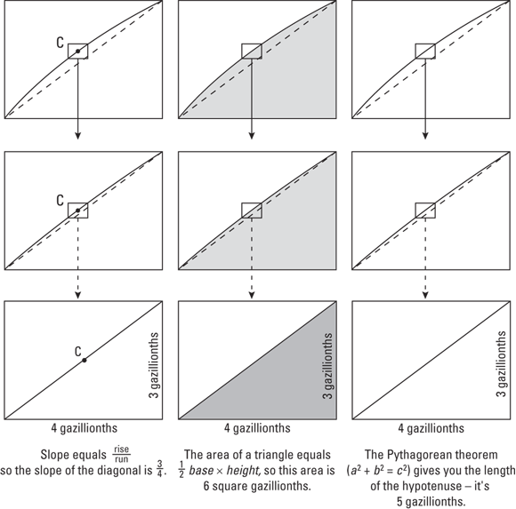
FIGURE 1-10: Zooming in to the sub, sub, sub … subatomic level.
Finally, the bottom row of Figure 1-10 shows the result after an “infinite” number of magnifications — sort of. You can think of the lengths 3 and 4 in the bottom row of rectangles as 3 and 4 millionths of an inch, no, make that 3 and 4 billionths of an inch, no, trillionths, no, gazillionths… .
After zooming in “forever,” the curve is perfectly straight, and now regular algebra and geometry formulas work.
For the diagram on the left in Figure 1-10, you can now use the regular slope formula from algebra to find the slope at point C. It’s exactly 3/4 — that’s the answer to the first question in Figure 1-9. This is how differentiation works.
For the diagram in the middle, the regular triangle formula from geometry gives an area of 6. So to get the total shaded area in Figure 1-9, you add the area of the thin rectangle under this triangle (the thin strip in Figure 1-9 shows the basic idea), repeat this process for all the other narrow strips, and then just add up all the little areas. This is how regular integration works.
For the diagram on the right, geometry’s Pythagorean theorem gives you a length of 5. Then to find the total length of the curve from A to B in Figure 1-9, you do the same thing for the other minute sections of the curve and then add up all the little lengths. This is how you calculate arc length (another integration problem).
Well, there you have it. Calculus uses the limit process to zoom in on a curve till it’s straight. After it’s straight, the rules of regular-old math apply. Calculus thus gives ordinary algebra and geometry the power to handle complicated problems involving changing quantities (which on a graph show up as curves). This explains why calculus has so many practical uses, because if there’s something you sure can count on — in addition to death and taxes — it’s that things are always changing.