Chapter 11
Using the Integral to Solve Problems
IN THIS CHAPTER
![]() Adding up the area between curves
Adding up the area between curves
![]() Figuring out volumes of weird shapes
Figuring out volumes of weird shapes
![]() Finding arc length
Finding arc length
As I say in Chapter 8, integration is basically adding up small pieces of something to get the total for the whole thing — really small pieces, actually, infinitely small pieces. Thus, the integral
tells you to add up all the little pieces of distance traveled during the 15-second interval from 5 to 20 seconds to get the total distance traveled during that interval. In all problems, the little piece after the integration symbol is always an expression in x (or other variable). For the above integral, for instance, the little piece of distance might be given by, say, ![]() . Then the definite integral
. Then the definite integral
would give you the total distance traveled. Your main challenge in this chapter is simply to come up with the algebraic expression for the little pieces you’re adding up. Before we begin the adding-up problems, I want to cover a couple other integration topics.
The Mean Value Theorem for Integrals and Average Value
The best way to understand the Mean Value Theorem for Integrals is with a diagram — look at Figure 11-1.

FIGURE 11-1: A visual “proof” of the mean value theorem for integrals.
The graph on the left in Figure 11-1 shows a rectangle whose area is clearly less than the area under the curve between 2 and 5. This rectangle has a height equal to the lowest point on the curve in the interval from 2 to 5. The middle graph shows a rectangle whose height equals the highest point on the curve. Its area is clearly greater than the area under the curve. By now you’re thinking, “Isn’t there a rectangle taller than the short one and shorter than the tall one whose area is the same as the area under the curve?” Of course. And this rectangle obviously crosses the curve somewhere in the interval. This so-called “mean value rectangle,” shown on the right, basically sums up the Mean Value Theorem for Integrals. It’s really just common sense. But here’s the mumbo jumbo.
 The Mean Value Theorem for Integrals: If
 ![]() is a continuous function on the closed interval [a, b], then there exists a number c in the closed interval such that
is a continuous function on the closed interval [a, b], then there exists a number c in the closed interval such that
The theorem basically just guarantees the existence of the mean value rectangle.
The area of the mean value rectangle — which is the same as the area under the curve — equals length times width, or base times height, right? So, if you divide its area, ![]() , by its base,
, by its base, ![]() , you get its height,
, you get its height, ![]() . This height is the average value of the function over the interval in question.
. This height is the average value of the function over the interval in question.
 Average Value: The average value of a function
 ![]() over a closed interval [a, b] is
over a closed interval [a, b] is
which is the height of the mean value rectangle.
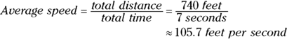
Here’s an example: What’s the average speed of a car between ![]() seconds and
seconds and ![]() seconds whose speed in feet per second is given by the function
seconds whose speed in feet per second is given by the function ![]() ? According to the definition of average value, this average speed is given by
? According to the definition of average value, this average speed is given by ![]() .
.
- Determine the area under the curve between 9 and 16.
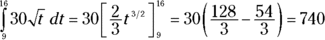
This area, by the way, is the total distance traveled from 9 to 16 seconds. Do you see why? Consider the mean value rectangle to answer this question. Its height is a speed (because the function values, or heights, are speeds) and its base is an amount of time, so its area is speed times time which equals distance.
- Divide this area, total distance, by the time interval from 9 to 16, namely 7.
The definition of average value tells you to multiply the total area by
 , which in this problem is
  , or
, or  . But because dividing by 7 is the same as multiplying by
  , you can divide like I do in this step. It makes more sense to think about these problems in terms of division: area equals base times height, so the height of the mean value rectangle equals its area divided by its base.
The Area between Two Curves
This is the first of seven topics in this chapter where your task is to come up with an expression for a little bit of something and then add up the bits by integrating. For this first problem type, the little bit is a narrow rectangle that sits on one curve and goes up to another. Here’s an example: Find the area between ![]() and
and ![]() from
from ![]() to
to ![]() . See Figure 11-2.
. See Figure 11-2.

FIGURE 11-2: The area between  and
and  from
from  to
to  .
.
To get the height of the representative rectangle in Figure 11-2, subtract the y-coordinate of its bottom from the y-coordinate of its top — that’s ![]() . Its base is the infinitesimal dx. So, because area equals height times base,
. Its base is the infinitesimal dx. So, because area equals height times base,
Now add up the areas of all rectangles from 0 to 1 by integrating:
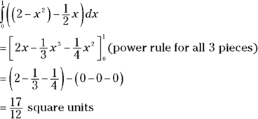
To make things a little more twisted, in the next problem the curves cross (see Figure 11-3). When this happens, you have to split the total shaded area into two separate regions before integrating. Find the area between ![]() and
and ![]() from
from ![]() to
to ![]() .
.
-
Determine where the curves cross.
They cross at (1, 1), so you’ve got two separate regions — one from 0 to 1 and another from 1 to 2.
-
Figure the area of the region on the left.
For this region,
 is above
  . So the height of a representative rectangle is
  , its area is height times base, or
  , and the area of the region is, therefore,
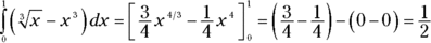
-
Figure the area of the region on the right.
Now,
 is above
  , so the height of a rectangle is
  and thus you’ve got
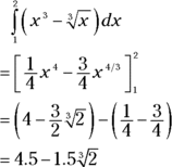
- Add up the areas of the two regions to get total area.

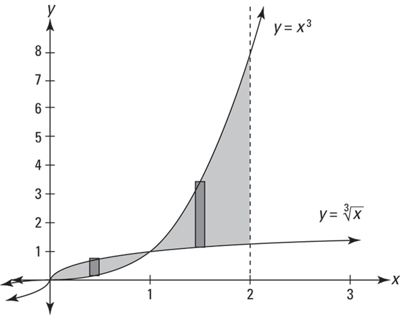
FIGURE 11-3: Who’s on top?
Volumes of Weird Solids
Integration enables you to calculate the volumes of shapes that you can’t get with basic geometry formulas.
The meat-slicer method
This metaphor is actually quite accurate. Picture a hunk of meat being cut into very thin slices on one of those deli meat slicers. That’s the basic idea here. You slice up a three-dimensional shape, then add up the volumes of the slices to determine the total volume.
Here’s a problem: What’s the volume of the solid whose length runs along the x-axis from 0 to ![]() and whose cross sections perpendicular to the x-axis are equilateral triangles such that the midpoints of their bases lie on the x-axis and their top vertices are on the curve
and whose cross sections perpendicular to the x-axis are equilateral triangles such that the midpoints of their bases lie on the x-axis and their top vertices are on the curve ![]() ? Is that a mouthful or what? This problem is almost harder to describe and to picture than it is to do. Take a look at this thing in Figure 11-4.
? Is that a mouthful or what? This problem is almost harder to describe and to picture than it is to do. Take a look at this thing in Figure 11-4.

FIGURE 11-4: One weird hunk of pastrami.
So what’s the volume?
-
Determine the area of any old cross section.
Each cross section is an equilateral triangle with a height of
 . If you do the geometry, you’ll see that its base is
  times its height, or
  (Hint: Half of an equilateral triangle is a
  triangle). So, the triangle’s area, given by
  is
is 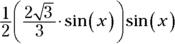 , or
, or  .
. -
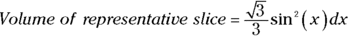
Find the volume of a representative slice.
The volume of a slice is just its cross-sectional area times its infinitesimal thickness, dx. So you’ve got its volume:
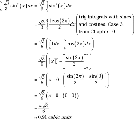
- Add up the volumes of the slices from 0 to
 by integrating.
The disk method
This technique is a special case of the meat slicer method that you use when the cross-sections are all circles. Find the volume of the solid — between ![]() and
and ![]() — generated by rotating the curve
— generated by rotating the curve ![]() about the x-axis. See Figure 11-5.
about the x-axis. See Figure 11-5.
-
Determine the area of any old cross section or representative disk.
Each cross section is a circle with a radius of
 . So, its area is given by the formula for the area of a circle,
  . Plugging
  into r gives you
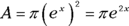
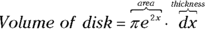
- Tack on a dx to get the volume of an infinitely thin representative disk.
- Add up the volumes of the disks from 2 to 3 by integrating.

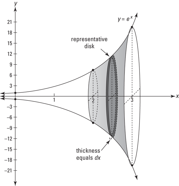
FIGURE 11-5: A sideways stack of disks.
The washer method
The only difference between the washer method and the disk method is that now each slice has a hole in its middle that you have to subtract. Take the area bounded by ![]() and
and ![]() , and generate a solid by revolving that area about the x-axis. See Figure 11-6.
, and generate a solid by revolving that area about the x-axis. See Figure 11-6.

FIGURE 11-6: A sideways stack of washers — just add up the volumes of all the washers.
So what’s the volume of this bowl-like shape?
-
Determine where the two curves intersect.
It should take very little trial and error to see that
 and
and  intersect at
  and
and  . So the solid in question spans the interval on the x-axis from 0 to 1.
 -
Figure the area of a thin cross-sectional washer.
Each slice has the shape of a washer — see Figure 11-7 — so its area equals the area of the entire circle minus the area of the hole.
The area of the circle minus the hole is
 , where R is the outer radius (the big radius) and r is the radius of the hole (the little radius). For this problem, the outer radius is
  and the radius of the hole is
  , so that gives you
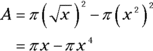
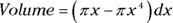
- Multiply this area by the thickness, dx, to get the volume of a representative washer.
- Add up the volumes of the even-thinner-than-paper-thin washers from 0 to 1 by integrating.
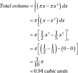
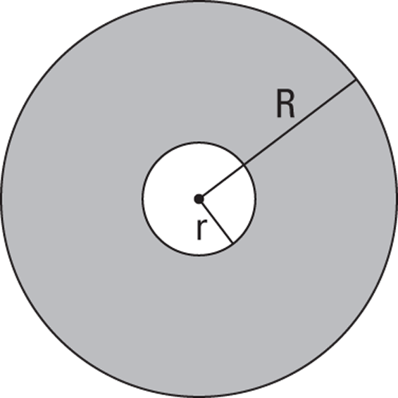
FIGURE 11-7: The shaded area equals  : The whole minus the hole — get it?
The matryoshka doll method
Now you’re going to cut up a solid into thin concentric cylinders and then add up the volumes of all the cylinders. It’s kinda like how those nested Russian (matryoshka) dolls fit inside each other. Or imagine a soup can that somehow has many paper labels, each one covering the one beneath it. Or picture one of those clothes de-linters with the sticky papers you peel off. Each soup can label or piece of sticky paper is a cylindrical shell — before you tear it off, of course. After you tear it off, it’s an ordinary rectangle.
Here’s a problem: A solid is generated by taking the area bounded by the x-axis, the lines ![]() ,
, ![]() , and
, and ![]() , and then revolving it about the y-axis. What’s its volume? See Figure 11-8.
, and then revolving it about the y-axis. What’s its volume? See Figure 11-8.
-
Determine the area of a representative cylindrical shell.
When picturing a representative shell, focus on one that’s in no place in particular. Figure 11-8 shows such a generic shell. Its radius is unknown, x, and its height is the height of the curve at x, namely
 . If, instead, you use a special shell like the outermost shell with a radius of 3, you’re more likely to make the mistake of thinking that a representative shell has some known radius like 3 or a known height like
  . Both the radius and the height are unknown. (This advice also applies to disk and washer problems.)
Each representative shell, like the soup can label or the sticky sheet from a de-linter, is just a rectangle whose area is, of course, length times width. The rectangular soup can label goes all the way around the can, so its length is the circumference of the can, namely
 ; the width of the label is the height of the can. So now you’ve got the general formula for the area of a representative shell:
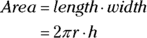
For the current problem, you plug in x for the radius and
 for the height, giving you the area of a representative shell:
- Multiply the area by the thickness of the shell, dx, to get its volume.

- Add up the volumes of all the shells from 2 to 3 by integrating.


FIGURE 11-8: A shape sort of like the Roman Coliseum and one of its representative shells.
 With the meat-slicer, disk, and washer methods, it’s usually pretty obvious what the limits of integration should be (recall that the limits of integration are, for example, the 1 and 5 in
 ![]() ). With cylindrical shells, however, it’s not always as clear. A tip: You integrate from the right edge of the smallest cylinder to the right edge of the biggest cylinder (like from 2 to 3 in the previous problem). And note that you never integrate from the left edge to the right edge of the biggest cylinder (like from
). With cylindrical shells, however, it’s not always as clear. A tip: You integrate from the right edge of the smallest cylinder to the right edge of the biggest cylinder (like from 2 to 3 in the previous problem). And note that you never integrate from the left edge to the right edge of the biggest cylinder (like from ![]() to 3).
to 3).
Arc Length
So far in this chapter, you’ve added up the areas of thin rectangles to get total area, and the volumes of thin slices or thin cylinders to get total volume. Now, you’re going to add up minute lengths along a curve, an “arc,” to get the whole length. The idea is to divide a length of curve into small sections, figure the length of each, and then add them all up. Figure 11-9 shows how each section of a curve is approximated by the hypotenuse of a tiny right triangle.

FIGURE 11-9: The Pythagorean Theorem,  , is the key to the arc length formula.
You can imagine that as you zoom in further and further, dividing the curve into more and more sections, the minute sections get straighter and straighter and the hypotenuses become better and better approximations of the curve. So, all you have to do is add up all the hypotenuses along the curve between your start and finish points. The lengths of the legs of each infinitesimal triangle are dx and dy, and thus the length of the hypotenuse — given by the Pythagorean Theorem — is
To add up all the hypotenuses from a to b along the curve, you just integrate:
A little tweaking and you have the formula for arc length. First, factor out a ![]() under the square root and simplify:
under the square root and simplify:

Now you take the square root of ![]() — that’s dx, of course — bring it outside the radical, and, voilà, you’ve got the formula.
— that’s dx, of course — bring it outside the radical, and, voilà, you’ve got the formula.
Arc Length: The arc length along a curve, ![]() , from a to b, is given by the following integral:
, from a to b, is given by the following integral:
The expression inside this integral is simply the length of a representative hypotenuse.
Try this: What’s the length along ![]() from
from ![]() to
to ![]() ?
?
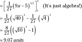
- Take the derivative of your function.
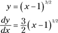
- Plug this into the formula and integrate.
(See how I got that? It’s the guess-and-check integration technique with the reverse power rule. The 4/9 is the tweak amount you need because of the coefficient 9/4.)
Improper Integrals
Definite integrals are improper when they go infinitely far up, down, right, or left. They go up or down infinitely far in problems like ![]() that have one or more vertical asymptotes. They go infinitely far to the right or left in problems like
that have one or more vertical asymptotes. They go infinitely far to the right or left in problems like ![]() or
or ![]() , where one or both of the limits of integration is infinite. It would make sense to use the term infinite instead of improper to describe these integrals, except that many of these “infinite” integrals have finite area. More about this in a minute.
, where one or both of the limits of integration is infinite. It would make sense to use the term infinite instead of improper to describe these integrals, except that many of these “infinite” integrals have finite area. More about this in a minute.
You solve both types of improper integrals by turning them into limit problems. Take a look at some examples.
Improper integrals with vertical asymptotes
A vertical asymptote may be at the edge of the area in question or in the middle of it.
A vertical asymptote at one of the limits of integration
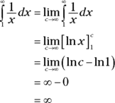
What’s the area under ![]() from 0 to 1? This function is undefined at x = 0, and it has a vertical asymptote there. So you’ve got to turn the definite integral into a limit:
from 0 to 1? This function is undefined at x = 0, and it has a vertical asymptote there. So you’ve got to turn the definite integral into a limit:
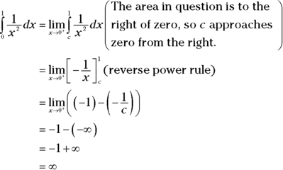
This area is infinite, which probably doesn’t surprise you because the curve goes up to infinity. But hold on to your hat — the next function also goes up to infinity at ![]() , but its area is finite!
, but its area is finite!
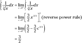
Find the area under ![]() from 0 to 1. This function is also undefined at
from 0 to 1. This function is also undefined at ![]() , so the solution process is the same as in the previous example.
, so the solution process is the same as in the previous example.
Convergence and Divergence: You say that an improper integral converges if the limit exists, that is, if the limit equals a finite number like in the second example. Otherwise, an improper integral is said to diverge — like in the first example. When an improper integral diverges, the area in question (or part of it) usually equals ![]() .
.
A vertical asymptote between the limits of integration
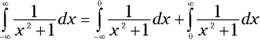
If the undefined point of the integrand is somewhere in between the limits of integration, you split the integral in two — at the undefined point — then turn each integral into a limit and go from there. Evaluate ![]() . This integrand is undefined at
. This integrand is undefined at ![]() .
.
- Split the integral in two at the undefined point.

-
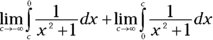
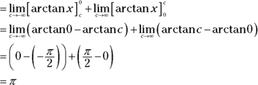
Turn each integral into a limit and evaluate.
For the
 integral, the area is to the left of zero, so c approaches zero from the left. For the
  integral, the area is to the right of zero, so c approaches zero from the right.
 If you fail to notice that an integral has an undefined point between the limits of integration, and you integrate the ordinary way, you may get the wrong answer. The above problem,
 ![]() , happens to work out right if you do it the ordinary way. However, if you do
, happens to work out right if you do it the ordinary way. However, if you do ![]() the ordinary way, not only do you get it wrong, you get the absurd answer of negative 2, even though the function is positive from
the ordinary way, not only do you get it wrong, you get the absurd answer of negative 2, even though the function is positive from ![]() . Don’t risk it.
. Don’t risk it.
If either part of the split-up integral diverges, the original integral diverges. You can’t get, say, ![]() for one part and
for one part and ![]() for the other part and add them up to get zero.
for the other part and add them up to get zero.
Improper integrals with infinite limits of integration
You do these improper integrals by turning them into limits where c approaches infinity or negative infinity. Here are two examples: ![]() and
and ![]() .
.
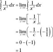
So this improper integral converges. In the next integral, the denominator is smaller — x instead of ![]() — and thus the fraction is bigger, so you’d expect
— and thus the fraction is bigger, so you’d expect ![]() to be bigger than
to be bigger than ![]() , which it is. But it’s not just bigger, it’s way, way bigger.
, which it is. But it’s not just bigger, it’s way, way bigger.
This improper integral diverges.
When both of the limits of integration are infinite, you split the integral in two and turn each part into a limit. Splitting up the integral at x = 0 is convenient because zero’s an easy number to deal with, but you can split it up anywhere. Zero may also seem like a good choice because it looks like it’s in the middle between ![]() . But that’s an illusion because there is no middle between
. But that’s an illusion because there is no middle between ![]() , or you could say that any point on the x-axis is the middle.
, or you could say that any point on the x-axis is the middle.
Here’s an example: ![]()
- Split the integral in two.
- Turn each part into a limit.
- Evaluate each part and add up the results.
If either “half” integral diverges, the whole diverges.