Chapter 8
Introduction to Integration
IN THIS CHAPTER
![]() Integrating — adding it all up
Integrating — adding it all up
![]() Approximating areas
Approximating areas
![]() Using the definite integral to get exact areas
Using the definite integral to get exact areas
If you’re still reading, I presume you survived differentiation (Chapters 4–7). Now you begin the second major calculus topic: integration. Just as two simple ideas lie at the heart of differentiation — rate (like miles per hour) and the slope of a curve — integration can also be understood in terms of two simple ideas: adding up small pieces of something and the area under a curve.
Integration: Just Fancy Addition
Say you want to determine the volume of the lamp’s base in Figure 8-1. Because no formula for the volume of such a weird shape exists, you can’t calculate the volume directly. You can, however, calculate the volume with integration. Imagine that the base is cut up into thin, horizontal slices, as shown on the right in Figure 8-1.

FIGURE 8-1: A lamp with a curvy base and the base cut into thin horizontal slices.
Do you see how each slice is shaped like a thin pancake? Now, because there is a formula for the volume of a pancake (a pancake is just a very short cylinder), you can determine the total volume of the base by simply calculating the volume of each pancake-shaped slice and then adding up the volumes. That’s integration in a nutshell.
What makes integration one of the great achievements in the history of mathematics is that — to stay with the lamp example — it gives you the exact volume of the lamp’s base by sort of cutting it into an infinite number of infinitely thin slices. If you cut the lamp into fewer than an infinite number of slices, you can get only a very good approximation of the volume because each slice will have a weird, curved edge which would cause a small error.
Integration has an elegant symbol: ![]() . You’ve probably seen it before. You can think of the integration symbol as an elongated S for “sum up.” So, for our lamp problem, you can write
. You’ve probably seen it before. You can think of the integration symbol as an elongated S for “sum up.” So, for our lamp problem, you can write
where dB means a little bit of the base — actually an infinitely small piece. So the equation just means that if you sum up all the little pieces of the base from the bottom to the top, the result is B, the volume of the whole base.
This is a bit oversimplified — I can hear the siren of the math police now — but it’s a good way to think about integration. By the way, thinking of dB as a little or infinitesimal piece of B is an idea you saw before with differentiation (see Chapter 4), where the derivative or slope, ![]() , is equal to the ratio of a little bit of y to a little bit of x, as you shrink the slope stair step down to an infinitesimal size — see Figure 8-2.
, is equal to the ratio of a little bit of y to a little bit of x, as you shrink the slope stair step down to an infinitesimal size — see Figure 8-2.

FIGURE 8-2: In the limit, 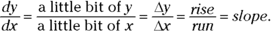
So, whenever you see something like
it just means that you add up all the little pieces of the mumbo jumbo from a to b to get the total of all of the mumbo jumbo from a to b. Or you might see something like
which means add up the little pieces of distance traveled between 0 and 20 seconds to get the total distance traveled in that time span.
To sum up — that’s a pun! — the mathematical expression to the right of the integration symbol always stands for a little bit of something, and integrating such an expression means to add up all the little pieces between some starting point and some ending point.
Finding the Area under a Curve
The most fundamental meaning of integration is to add up. And when you depict integration on a graph, you can see the adding up process as a summing up of little bits of area to arrive at the total area under a curve. Consider Figure 8-3.
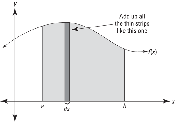
FIGURE 8-3: Integrating f(x) from a to b means finding the area under the curve between a and b.
The shaded area in Figure 8-3 can be calculated with the following integral:
Look at the thin rectangle in Figure 8-3. It has a height of ![]() and a width of dx (a little bit of x), so its area (length × width, of course) is given by
and a width of dx (a little bit of x), so its area (length × width, of course) is given by ![]() . The above integral tells you to add up the areas of all the narrow rectangular strips between a and b under the curve
. The above integral tells you to add up the areas of all the narrow rectangular strips between a and b under the curve ![]() . As the strips get narrower and narrower, you get a better and better estimate of the area. The power of integration lies in the fact that it gives you the exact area by sort of adding up an infinite number of infinitely thin rectangles.
. As the strips get narrower and narrower, you get a better and better estimate of the area. The power of integration lies in the fact that it gives you the exact area by sort of adding up an infinite number of infinitely thin rectangles.
If you’re doing a problem where both the x and y axes are labeled in a unit of length, say, feet, then each thin rectangle measures so many feet by so many feet, and its area — length × width — is some number of square feet. In this case, when you integrate to get the total area under the curve between a and b, your final answer will be an amount of — what else? — area. But you can use this adding-up-areas-of-rectangles scheme to add up tiny bits of anything — distance, volume, or energy, for example. In other words, the area under the curve doesn’t have to stand for an actual area.
If, for example, the units on the x-axis are hours and the y-axis is labeled in miles per hour, then, because rate × time = distance, the area of each rectangle represents an amount of distance, and the total area gives you the total distance traveled during the given time interval. Or if the x-axis is labeled in hours and the y-axis in kilowatts of electrical power — in which case the curve gives power usage as a function of time — then the area of each rectangular strip (kilowatts × hours) represents a number of kilowatt-hours of energy. In that case, the total area under the curve gives you the total number of kilowatt-hours of energy consumption between two points in time.
Dealing with negative area
In the examples involving volume, distance, and energy (see previous two sections), you’re adding up positive bits of something. This is common with practical problems because you can’t, say, have a negative volume of water or use a negative number of kilowatt-hours. However, you will sometimes integrate functions that go into the negatives — that’s below the x-axis. Here’s what you do.
 When using integration to calculate area, area below the x-axis counts as negative area. The total area between a and b for some curve
 ![]() — given by the integral
— given by the integral ![]() — is really a net area where the total area below the x-axis (and above the curve) is subtracted from the total area above the x-axis (and below the curve).
— is really a net area where the total area below the x-axis (and above the curve) is subtracted from the total area above the x-axis (and below the curve).
Approximating Area
Before explaining how to calculate exact areas, I want to show you how to approximate areas. The approximation method is useful not only because it lays the groundwork for the exact method — integration — but because for some curves, integration is impossible, and an approximation of area is the best you can do.
Approximating area with left sums
Say you want the exact area under the curve ![]() between 0 and 3. See the shaded area on the graph on the left in Figure 8-4.
between 0 and 3. See the shaded area on the graph on the left in Figure 8-4.
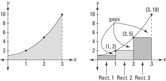
FIGURE 8-4: The exact area under  between 0 and 3 (left) is approximated by the area of three rectangles (right).
You can get a rough estimate of the area by drawing three rectangles under the curve, as shown on the right in Figure 8-4, and then adding up their areas.
The rectangles in Figure 8-4 represent a so-called left sum because the upper left corner of each rectangle touches the curve. Each rectangle has a width of 1 and the height of each is given by the height of the function at the rectangle’s left edge. So, rectangle number 1 has a height of ![]() ; its area (
; its area (![]() ) is thus
) is thus ![]() , or 1. Rectangle 2 has a height of
, or 1. Rectangle 2 has a height of ![]() , so its area is
, so its area is ![]() , or 2. And rectangle 3 has a height of
, or 2. And rectangle 3 has a height of ![]() , so its area is
, so its area is ![]() , or 5. Adding the areas gives you
, or 5. Adding the areas gives you ![]() , or 8. This is an underestimate of the total area under the curve because of the gaps between the rectangles and the curve.
, or 8. This is an underestimate of the total area under the curve because of the gaps between the rectangles and the curve.
For a better estimate, double the number of rectangles to six. Figure 8-5 shows six “left” rectangles under the curve and also how they begin to fill up the three gaps you see in Figure 8-4.
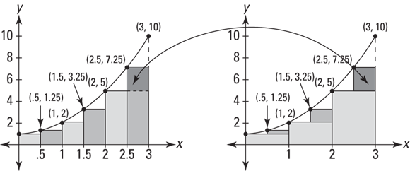
FIGURE 8-5: Six “left” rectangles approximate the area under  .
.
See the three small, darker shaded rectangles in the graph on the right in Figure 8-5? They sit on top of the three rectangles from Figure 8-4, and they represent how much the area estimate has improved by using six rectangles instead of three.
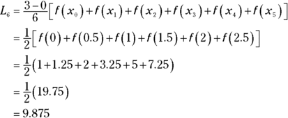
Now total up the areas of the six rectangles. Each has a width of 0.5 and the heights are ![]() and so on. I’ll spare you the math. Here’s the total:
and so on. I’ll spare you the math. Here’s the total: ![]() . This is a better estimate, but it’s still an underestimate because of the six small gaps you can see on the left graph in Figure 8-5.
. This is a better estimate, but it’s still an underestimate because of the six small gaps you can see on the left graph in Figure 8-5.
Table 8-1 shows the area estimates given by 3, 6, 12, 24, 48, 96, 192, and 384 rectangles. You don’t have to double the rectangles each time — you can use any number of rectangles you want. I just like the doubling scheme because, with each doubling, the gaps are plugged up more and more in the way shown in Figure 8-5.
TABLE 8-1 Estimates of the Area under ![]() Given by Increasing Numbers of “Left” Rectangles
Given by Increasing Numbers of “Left” Rectangles
Number of Rectangles |
Area Estimate |
|
3 6 12 24 48 96 192 384 |
8 9.875 ~10.906 ~11.445 ~11.721 ~11.860 ~11.930 ~11.965 |
 The Left Rectangle Rule: You can approximate the exact area under a curve between a and b,
 ![]() , with a sum of left rectangles given by the following formula. In general, the more rectangles, the better the estimate.
, with a sum of left rectangles given by the following formula. In general, the more rectangles, the better the estimate.
Where n is the number of rectangles, ![]() is the width of each one, and the function values are the heights of the rectangles.
is the width of each one, and the function values are the heights of the rectangles.
Look back to the six rectangles shown in Figure 8-5. The width of each rectangle equals the length of the total span from 0 to 3 (which of course is ![]() , or 3) divided by the number of rectangles, 6. That’s what the
, or 3) divided by the number of rectangles, 6. That’s what the ![]() does in the formula.
does in the formula.
What about those xs with the subscripts? The x-coordinate of the left edge of rectangle 1 in Figure 8-5 is ![]() , the right edge of rectangle 1 (the same as the left edge of rectangle 2) is at
, the right edge of rectangle 1 (the same as the left edge of rectangle 2) is at ![]() , the right edge of rectangle 2 is at
, the right edge of rectangle 2 is at ![]() , the right edge of rectangle 3 is at
, the right edge of rectangle 3 is at ![]() , and so on up to the right edge of rectangle 6, at
, and so on up to the right edge of rectangle 6, at ![]() . For the six rectangles in Figure 8-5,
. For the six rectangles in Figure 8-5, ![]() is 0,
is 0, ![]() is 0.5,
is 0.5, ![]() is 1,
is 1, ![]() is 1.5,
is 1.5, ![]() is 2,
is 2, ![]() is 2.5, and
is 2.5, and ![]() is 3. The heights of the six left rectangles in Figure 8-5 occur at their left edges, which are at
is 3. The heights of the six left rectangles in Figure 8-5 occur at their left edges, which are at ![]() through
through ![]() . You don’t use the right edge of the last rectangle,
. You don’t use the right edge of the last rectangle, ![]() , in a left sum. That’s why the list of function values in the formula stops at
, in a left sum. That’s why the list of function values in the formula stops at ![]() .
.
Here’s how to use the formula for the six rectangles in Figure 8-5:
Had I distributed the width of 1/2 to each of the heights after the third line in that solution, you’d see the sum of the areas of the rectangles — seen just before Figure 8-5. The formula uses the shortcut of first adding up the heights and then multiplying by the width.
Approximating area with right sums
Now let’s estimate the same area under ![]() from 0 to 3 with right rectangles. This method works just like the left sum method except that each rectangle is drawn so that its right upper corner touches the curve. See Figure 8-6.
from 0 to 3 with right rectangles. This method works just like the left sum method except that each rectangle is drawn so that its right upper corner touches the curve. See Figure 8-6.

FIGURE 8-6: Three right rectangles used to approximate the area under  .
.
The heights of the three rectangles in Figure 8-6 are given by the function values at their right edges: ![]() , and
, and ![]() . Each rectangle has a width of 1, so the areas are 2, 5, and 10, which total 17. Table 8-2 shows the improving estimates you get with more and more right rectangles.
. Each rectangle has a width of 1, so the areas are 2, 5, and 10, which total 17. Table 8-2 shows the improving estimates you get with more and more right rectangles.
TABLE 8-2 Estimates of the Area under ![]() Given by Increasing Numbers of “Right” Rectangles
Given by Increasing Numbers of “Right” Rectangles
Number of Rectangles |
Area Estimate |
|
3 6 12 24 48 96 192 384 |
17 14.375 ~13.156 ~12.570 ~12.283 ~12.141 ~12.070 ~12.035 |
The Right Rectangle Rule: You can approximate the exact area under a curve between a and b, ![]() , with a sum of right rectangles given by the following formula. In general, the more rectangles, the better the estimate.
, with a sum of right rectangles given by the following formula. In general, the more rectangles, the better the estimate.
where n is the number of rectangles, ![]() is the width of each, and the function values are the heights of the rectangles.
is the width of each, and the function values are the heights of the rectangles.
If you compare this formula to the one for a left rectangle sum, you get the complete picture about those subscripts. The two formulas are the same except for one thing. Look at the sums of the function values in both formulas. The right sum formula has one value, ![]() , that the left sum formula doesn’t have, and the left sum formula has one value,
, that the left sum formula doesn’t have, and the left sum formula has one value, ![]() , that the right sum formula doesn’t have. All the function values between those two appear in both formulas. You can get a handle on this by comparing the three left rectangles from Figure 8-4 to the three right rectangles from Figure 8-6. Their areas and totals, which we calculated earlier, are
, that the right sum formula doesn’t have. All the function values between those two appear in both formulas. You can get a handle on this by comparing the three left rectangles from Figure 8-4 to the three right rectangles from Figure 8-6. Their areas and totals, which we calculated earlier, are
Three left rectangles:
Three right rectangles:
The sums of the areas are the same except for the left-most left rectangle and the right-most right rectangle. Both sums include the rectangles with areas 2 and 5. Look at how the rectangles are constructed — the second and third rectangles in Figure 8-4 are the same as the first and second rectangles in Figure 8-6.
Approximating area with midpoint sums
A third way to approximate areas with rectangles is to make each rectangle cross the curve at the midpoint of its top side. A midpoint sum is a much better estimate of area than either a left or a right sum. Figure 8-7 shows why.
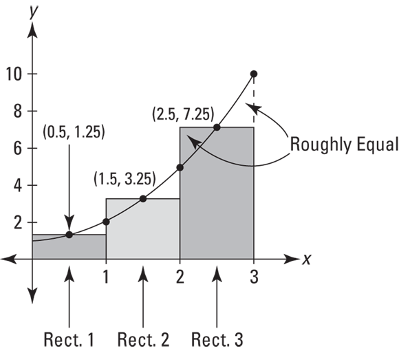
FIGURE 8-7: Three midpoint rectangles give you a much better estimate of the area under  .
.
You can see in Figure 8-7 that the part of each rectangle that’s above the curve looks about the same size as the gap between the rectangle and the curve. A midpoint sum produces such a good estimate because these two errors roughly cancel out each other.
For the three rectangles in Figure 8-8, the widths are 1 and the heights are ![]() ,
, ![]() , and
, and ![]() . The total area comes to 11.75. Table 8-3 lists the midpoint sums for the same number of rectangles used in Tables 8-1 and 8-2.
. The total area comes to 11.75. Table 8-3 lists the midpoint sums for the same number of rectangles used in Tables 8-1 and 8-2.
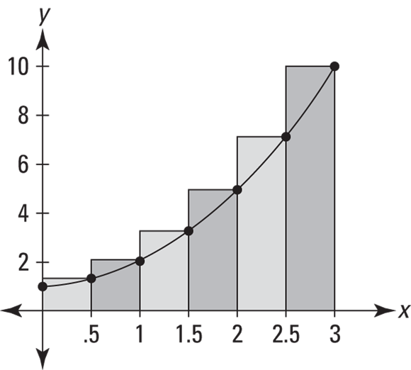
FIGURE 8-8: Six right rectangles approximate the area under  between 0 and 3.
TABLE 8-3 Estimates of the Area under ![]() Given by Increasing Numbers of “Midpoint” Rectangles
Given by Increasing Numbers of “Midpoint” Rectangles
Number of Rectangles |
Area Estimate |
|
3 6 12 24 48 96 192 384 |
11.75 11.9375 ~11.9844 ~11.9961 ~11.9990 ~11.9998 ~11.9999 ~11.99998 |
Sorry to give away the ending, but you’ll soon see that the exact area is 12. And to see how much faster the midpoint approximations approach the exact answer of 12 than the left or right approximations, compare the three tables. The error with 6 midpoint rectangles is about the same as the error with 192 left or right rectangles!
The Midpoint Rule: You can approximate the exact area under a curve between a and b, ![]() , with a sum of midpoint rectangles given by the following formula. In general, the more rectangles, the better the estimate.
, with a sum of midpoint rectangles given by the following formula. In general, the more rectangles, the better the estimate.
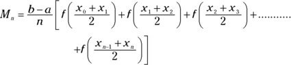
where n is the number of rectangles, ![]() is the width of each, and the function values are the heights of the rectangles.
is the width of each, and the function values are the heights of the rectangles.
The left, right, and midpoint sums are called Riemann sums after the great German mathematician G. F. B. Riemann (1826–66).
Summation Notation
For adding up long series of numbers like the rectangle areas in a left, right, or midpoint sum, summation or sigma notation is handy.
Summing up the basics
Say you wanted to add up the first 100 multiples of 5 — that’s from 5 to 500. You could write out the sum like this:
But with sigma notation, the sum is much more condensed.
This notation just tells you to plug 1 in for the i in 5i, then plug 2 into the i in 5i, then 3, then 4, all the way up to 100. Then you add up the results. So that’s ![]() plus
plus ![]() plus
plus ![]() , and so on, up to
, and so on, up to ![]() . It’s the same thing as writing out the sum the long way. By the way, the letter i has no significance. You can write the sum with a j,
. It’s the same thing as writing out the sum the long way. By the way, the letter i has no significance. You can write the sum with a j, ![]() , or any other letter you like.
, or any other letter you like.
Here’s one more. If you want to add up ![]()
![]() , you can write the sum with sigma notation as follows:
, you can write the sum with sigma notation as follows:
Writing Riemann sums with sigma notation
You can use sigma notation to write out the right-rectangle sum for the curve ![]() from the “Approximating Area” sections. Recall the formula for a right sum from the “Approximating area with right sums” section:
from the “Approximating Area” sections. Recall the formula for a right sum from the “Approximating area with right sums” section:
Here’s the same formula written with sigma notation:
Now work this out for the six right rectangles in Figure 8-8. You’re figuring the area under ![]() between 0 and 3 with six rectangles, so the width of each,
between 0 and 3 with six rectangles, so the width of each, ![]() . So now you’ve got
. So now you’ve got
Now, because the width of each rectangle is ![]() , the right edges of the six rectangles fall on the first six multiples of
, the right edges of the six rectangles fall on the first six multiples of ![]() : 0.5, 1, 1.5, 2, 2.5, and 3. These numbers are the x-coordinates of the six points
: 0.5, 1, 1.5, 2, 2.5, and 3. These numbers are the x-coordinates of the six points ![]() through
through ![]() ; they can be generated by the expression
; they can be generated by the expression ![]() , where i equals 1 through 6. You can check that this works by plugging 1 in for i in
, where i equals 1 through 6. You can check that this works by plugging 1 in for i in ![]() , then 2, then 3, up to 6. So now you can replace the
, then 2, then 3, up to 6. So now you can replace the ![]() in the formula with
in the formula with ![]() , giving you
, giving you
Our function, ![]() so
so ![]() , and so now you can write
, and so now you can write
If you plug 1 into i, then 2, 3, up to 6 and do the math, you get the sum of the areas of the rectangles in Figure 8-8. This sigma notation is just a fancy way of writing the sum of the six rectangles.
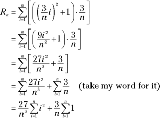
Are we having fun? Hold on, it gets worse. Now you’re going to write out the general sum for an unknown number (n) of right rectangles. The total span of the area in question is 3, right? You divide this span by the number of rectangles to get the width of each rectangle. With 6 rectangles, the width of each is ![]() ; with n rectangles, the width of each is
; with n rectangles, the width of each is ![]() . And the right edges of the n rectangles are generated by
. And the right edges of the n rectangles are generated by ![]() , for i equals 1 through n. That gives you
, for i equals 1 through n. That gives you
Or, because ![]() ,
,
For this last step, you pull the ![]() and the
and the ![]() through the summation signs — you’re allowed to pull out anything except for a function of i, the so-called index of summation. Also, the second summation in the last step has just a 1 after it and no i. So there’s nowhere to plug in the values of i. No worries — all you do is add up n 1s, which equals n (I do this in a minute).
through the summation signs — you’re allowed to pull out anything except for a function of i, the so-called index of summation. Also, the second summation in the last step has just a 1 after it and no i. So there’s nowhere to plug in the values of i. No worries — all you do is add up n 1s, which equals n (I do this in a minute).
With sleight of hand, you’re now going to turn the previous Riemann sum into a formula in terms of n. The sum of the first n square numbers, ![]() , equals
, equals ![]() (a formula you might want to memorize). So, you can substitute that expression for
(a formula you might want to memorize). So, you can substitute that expression for ![]() in the last line of the sigma notation solution, and at the same time substitute n for
in the last line of the sigma notation solution, and at the same time substitute n for ![]() :
:
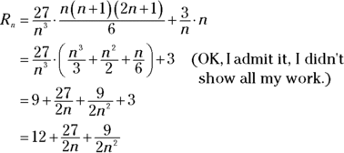
The end. Finally! This is the formula for the area of n right rectangles between 0 and 3 under the function ![]() . You can use this formula to produce the results given in Table 8-2. But once you’ve got such a formula, it’d be kind of pointless to produce a table of approximate areas, because you can use the formula to determine the exact area. I get to that in the next section.
. You can use this formula to produce the results given in Table 8-2. But once you’ve got such a formula, it’d be kind of pointless to produce a table of approximate areas, because you can use the formula to determine the exact area. I get to that in the next section.
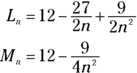
But first, here are the formulas for n left rectangles and n midpoint rectangles between 0 and 3 under the function ![]() . These formulas generate the area approximations in Tables 8-1 and 8-3.
. These formulas generate the area approximations in Tables 8-1 and 8-3.
Finding Exact Area with the Definite Integral
As you saw with the left, right, and midpoint rectangles in the “Approximating Area” sections, the more rectangles you have, the better the approximation. So, “all” you have to do to get the exact area under a curve is to use an infinite number of rectangles. Now, you can’t really do that, but with the fantastic invention of limits, this is sort of what happens. Here’s the definition of the definite integral that’s used to compute exact areas.
The Definite Integral (“simple” definition): The exact area under a curve between a and b is given by the definite integral, which is defined as the limit of a Riemann sum:
Is that a thing of beauty or what? The summation above is identical to the formula for n right rectangles, ![]() , from a few pages back. The only difference is that you take the limit of that formula as the number of rectangles approaches infinity.
, from a few pages back. The only difference is that you take the limit of that formula as the number of rectangles approaches infinity.
This definition of the definite integral is a simple version based on the right rectangle formula. I’ll skip the more complicated real-McCoy definition because you’ll never need to use it. All Riemann sums have the same limit — it doesn’t matter what type of rectangles you use — so you might as well use this right-rectangle definition.
Here, finally, is the exact area under ![]() between 0 and 3:
between 0 and 3:
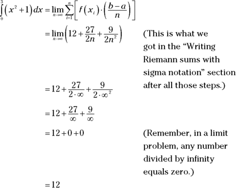
Big surprise.