Chapter 9
Integration: Backwards Differentiation
IN THIS CHAPTER
![]() Antidifferentiating — putting ’er in reverse
Antidifferentiating — putting ’er in reverse
![]() Using the area function
Using the area function
![]() Getting familiar with the Fundamental Theorem of Calculus
Getting familiar with the Fundamental Theorem of Calculus
Chapter 8 shows you the hard way to calculate the area under a curve using the formal definition of integration — the limit of a Riemann sum. In this chapter, I do it the easy way, taking advantage of one of the most important discoveries in mathematics — that integration is just differentiation in reverse.
Antidifferentiation: Reverse Differentiation
Antidifferentiation is just differentiation backwards. The derivative of sin x is cos x, so the antiderivative of cos x is sin x; the derivative of ![]() is
is ![]() , so the antiderivative of
, so the antiderivative of ![]() is
is ![]() — you just go backwards … with one twist: The derivative of
— you just go backwards … with one twist: The derivative of ![]() is also
is also ![]() , as is the derivative of
, as is the derivative of ![]() . Any function of the form
. Any function of the form ![]() , where C is any number, has a derivative of
, where C is any number, has a derivative of ![]() . So, every such function is an antiderivative of
. So, every such function is an antiderivative of ![]() .
.
 The Indefinite Integral: The indefinite integral of a function
 ![]() , written as
, written as ![]() , is the family of all antiderivatives of the function. For example, because the derivative of
, is the family of all antiderivatives of the function. For example, because the derivative of ![]() is
is ![]() , the indefinite integral of
, the indefinite integral of ![]() is
is ![]() , and you write
, and you write
You may recognize this integration symbol, ![]() , from the definite integral in Chapter 8. The definite integral symbol, however, contains two little numbers like
, from the definite integral in Chapter 8. The definite integral symbol, however, contains two little numbers like ![]() that tell you to compute the area of a function between the two numbers, called the limits of integration. The naked version of the symbol,
that tell you to compute the area of a function between the two numbers, called the limits of integration. The naked version of the symbol, ![]() , indicates an indefinite integral or an antiderivative. This chapter is about the intimate connection between these two symbols.
, indicates an indefinite integral or an antiderivative. This chapter is about the intimate connection between these two symbols.
Figure 9-1 shows the family of antiderivatives of the parabola ![]() , namely
, namely ![]() . Note that this family of curves has an infinite number of curves. They go up and down forever and are infinitely dense. The vertical gap of 2 units between each curve in Figure 9-1 is just a visual aid.
. Note that this family of curves has an infinite number of curves. They go up and down forever and are infinitely dense. The vertical gap of 2 units between each curve in Figure 9-1 is just a visual aid.

FIGURE 9-1: The family of curves  . All these functions have the same derivative,
  .
.
The top curve on the graph is ![]() ; the one below it is
; the one below it is ![]() ; the bottom one is
; the bottom one is ![]() . By the power rule, these three functions, as well as all the others in this family of functions, have a derivative of
. By the power rule, these three functions, as well as all the others in this family of functions, have a derivative of ![]() . Now consider the slope of each of the curves where x equals 1 (see the tangent lines drawn on the curves). The derivative of each curve is
. Now consider the slope of each of the curves where x equals 1 (see the tangent lines drawn on the curves). The derivative of each curve is ![]() , so when x equals 1, the slope of each curve is
, so when x equals 1, the slope of each curve is ![]() , or 3. Thus, all these little tangent lines are parallel. No matter what x-value you pick, tangent lines like this would be parallel. This is the visual way to understand why each of these curves has the same derivative, and, thus, why each curve is an antiderivative of the same function.
, or 3. Thus, all these little tangent lines are parallel. No matter what x-value you pick, tangent lines like this would be parallel. This is the visual way to understand why each of these curves has the same derivative, and, thus, why each curve is an antiderivative of the same function.
The Annoying Area Function
This topic is pretty tricky. Put on your thinking cap. Say you’ve got any old function, ![]() . Imagine that at some t-value, call it s, you draw a fixed vertical line. See Figure 9-2.
. Imagine that at some t-value, call it s, you draw a fixed vertical line. See Figure 9-2.

FIGURE 9-2: Area under f between s and x is swept out by the moving line at x.
Then you take a movable vertical line, starting at the same point, s (for starting point), and drag it to the right, sweeping out a larger and larger area under the curve. This area is a function of x, the position of the moving line. In symbols, you write
Note that t is the input variable in ![]() instead of x because x is already taken — it’s the input variable in
instead of x because x is already taken — it’s the input variable in ![]() . The subscript f in
. The subscript f in ![]() indicates that
indicates that ![]() is the area function for the particular curve f or
is the area function for the particular curve f or ![]() . The dt is a little increment along the t-axis — actually an infinitesimally small increment.
. The dt is a little increment along the t-axis — actually an infinitesimally small increment.
Here’s a simple example to make sure you’ve got a handle how an area function works. Say you’ve got the simple function, ![]() — that’s a horizontal line at
— that’s a horizontal line at ![]() . If you sweep out area beginning at
. If you sweep out area beginning at ![]() , you get the following area function:
, you get the following area function:
You can see that the area swept out from 3 to 4 is 10 because, in dragging the line from 3 to 4, you sweep out a rectangle with a width of 1 and a height of 10, which has an area of 1 times 10, or 10. See Figure 9-3.

FIGURE 9-3: Area under  between 3 and x is swept out by the moving vertical line at x.
So, ![]() , the area swept out as you hit 4, equals 10.
, the area swept out as you hit 4, equals 10. ![]() equals 20 because when you drag the line to 5, you’ve swept out a rectangle with a width of 2 and height of 10, which has an area of 2 times 10, or 20.
equals 20 because when you drag the line to 5, you’ve swept out a rectangle with a width of 2 and height of 10, which has an area of 2 times 10, or 20. ![]() equals 30, and so on.
equals 30, and so on.
Now, imagine that you drag the line across at a rate of one unit per second. You start at ![]() , and you hit 4 at 1 second, 5 at 2 seconds, 6 at 3 seconds, and so on. How much area are you sweeping out per second? Ten square units per second because each second you sweep out another 1-by-10 rectangle. Notice — this is huge — that because the width of each rectangle you sweep out is 1, the area of each rectangle — given by height times width — is the same as its height because anything times 1 equals itself.
, and you hit 4 at 1 second, 5 at 2 seconds, 6 at 3 seconds, and so on. How much area are you sweeping out per second? Ten square units per second because each second you sweep out another 1-by-10 rectangle. Notice — this is huge — that because the width of each rectangle you sweep out is 1, the area of each rectangle — given by height times width — is the same as its height because anything times 1 equals itself.
Okay, are you sitting down? You’ve reached another one of the big Ah ha! moments in the history of mathematics. Recall that a derivative is a rate. So, because the rate at which the previous area function grows is 10 square units per second, you can say its derivative equals 10. Thus, you can write
Here’s the critical thing: This rate or derivative of 10 is the same as the original function ![]() because as you go across 1 unit, you sweep out a rectangle that has an area of 10, the height of the function.
because as you go across 1 unit, you sweep out a rectangle that has an area of 10, the height of the function.
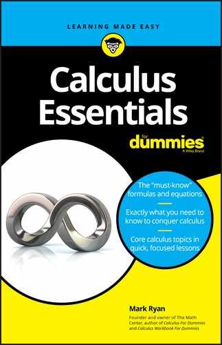
This works for any function, not just horizontal lines. Look at the function ![]() and its area function
and its area function ![]() that sweeps out area beginning at
that sweeps out area beginning at ![]() in Figure 9-4.
in Figure 9-4.
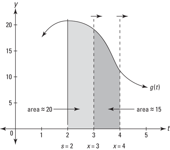
FIGURE 9-4: Area under g between 2 and x is swept out by the moving vertical line at x.
You can see that ![]() is about 20 because the area swept out between 2 and 3 has a width of 1 and the curved top of the “rectangle” has an average height of about 20. So, during this interval, the rate of growth of
is about 20 because the area swept out between 2 and 3 has a width of 1 and the curved top of the “rectangle” has an average height of about 20. So, during this interval, the rate of growth of ![]() is about 20 square units per second. Between 3 and 4, you sweep out about 15 square units of area because that’s roughly the average height of
is about 20 square units per second. Between 3 and 4, you sweep out about 15 square units of area because that’s roughly the average height of ![]() between 3 and 4. So, during second number two — the interval from
between 3 and 4. So, during second number two — the interval from ![]() to
to ![]() — the rate of growth of
— the rate of growth of ![]() is about 15.
is about 15.
The rate of area being swept out under a curve by an area function at a given x-value is equal to the height of the curve at that x-value.
The Fundamental Theorem
Sound the trumpets! Now that you’ve seen the connection between the rate of growth of an area function and the height of the given curve, you’re ready for what some say is one of the most important theorems in the history of mathematics:
The Fundamental Theorem of Calculus: Given an area function ![]() that sweeps out area under
that sweeps out area under ![]() ,
,
the rate at which area is being swept out is equal to the height of the original function. So, because the rate is the derivative, the derivative of the area function equals the original function:
Because ![]() , you can also write the above equation as follows:
, you can also write the above equation as follows:
Now, because the derivative of ![]() is
is ![]() ,
, ![]() is by definition an antiderivative of
is by definition an antiderivative of ![]() . Check out how this works by returning to the simple function from the previous section,
. Check out how this works by returning to the simple function from the previous section, ![]() , and its area function,
, and its area function, ![]() .
.
According to the Fundamental Theorem, ![]() . Thus
. Thus ![]() must be an antiderivative of 10; in other words,
must be an antiderivative of 10; in other words, ![]() is a function whose derivative is 10. Because any function of the form
is a function whose derivative is 10. Because any function of the form ![]() , where C is a number, has a derivative of 10, the antiderivative of 10 is
, where C is a number, has a derivative of 10, the antiderivative of 10 is ![]() . The particular number C depends on your choice of s, the point where you start sweeping out area. For a particular choice of s, the area function will be the one function (out of all the functions in the family of curves
. The particular number C depends on your choice of s, the point where you start sweeping out area. For a particular choice of s, the area function will be the one function (out of all the functions in the family of curves ![]() ) that crosses the x-axis at s. To figure out C, set the antiderivative equal to zero, plug the value of s into x, and solve for C.
) that crosses the x-axis at s. To figure out C, set the antiderivative equal to zero, plug the value of s into x, and solve for C.
For this function with an antiderivative of ![]() , if you start sweeping out area at, say,
, if you start sweeping out area at, say, ![]() , then
, then ![]() , so
, so ![]() , and thus
, and thus ![]() , or just 10x. If instead you start sweeping out area at
, or just 10x. If instead you start sweeping out area at ![]() and define a new area function,
and define a new area function, ![]() , then
, then ![]() , so C equals 20 and
, so C equals 20 and ![]() is thus
is thus ![]() . This area function is 20 more than
. This area function is 20 more than ![]() , which starts at
, which starts at ![]() , because if you start at
, because if you start at ![]() , you’ve already swept out an area of 20 by the time you get to zero.
, you’ve already swept out an area of 20 by the time you get to zero.
And if you start sweeping out area at ![]() ,
, ![]() , so
, so ![]() and the area function is
and the area function is ![]() . This function is 30 less than on
. This function is 30 less than on ![]() because with
because with ![]() , you lose the 3-by-10 rectangle between 0 and 3 that
, you lose the 3-by-10 rectangle between 0 and 3 that ![]() has.
has.
 The area swept out under the horizontal line
 ![]() , from some number s to x, is given by an antiderivative of 10, namely
, from some number s to x, is given by an antiderivative of 10, namely ![]() , where the value of C depends on where you start sweeping out area.
, where the value of C depends on where you start sweeping out area.
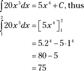
For the next example, look again at the parabola ![]() , our friend from Chapter 8, and the discussion of Riemann sums. Flip back to Figure 8-5. Now you can finally compute the exact area (from 0 to 3) in that graph the easy way.
, our friend from Chapter 8, and the discussion of Riemann sums. Flip back to Figure 8-5. Now you can finally compute the exact area (from 0 to 3) in that graph the easy way.
The area function for sweeping out area under ![]() is
is ![]() . By the Fundamental Theorem,
. By the Fundamental Theorem, ![]() , and so
, and so ![]() is an antiderivative of
is an antiderivative of ![]() . Any function of the form
. Any function of the form ![]() has a derivative of
has a derivative of ![]() (try it), so that’s the antiderivative. For Figure 8-5, you want to sweep out area beginning at 0, so
(try it), so that’s the antiderivative. For Figure 8-5, you want to sweep out area beginning at 0, so ![]() . Plug 0 into the antiderivative and solve for C:
. Plug 0 into the antiderivative and solve for C: ![]() , so
, so ![]() , and thus
, and thus
The area swept out from 0 to 3 — which we did the hard way in Chapter 8 by computing the limit of a Riemann sum — is simply ![]() :
:
That was much less work than doing it the hard way. And after you know the area function that starts at zero, ![]() , it’s a snap to figure the area of other sections under the parabola that don’t start at zero. Say you want the area under the parabola between 2 and 3. You can compute it by subtracting the area between 0 and 2 from the area between 0 and 3. You just figured the area between 0 and 3 — that’s 12. And the area between 0 and 2 is
, it’s a snap to figure the area of other sections under the parabola that don’t start at zero. Say you want the area under the parabola between 2 and 3. You can compute it by subtracting the area between 0 and 2 from the area between 0 and 3. You just figured the area between 0 and 3 — that’s 12. And the area between 0 and 2 is ![]() . So the area between 2 and 3 is
. So the area between 2 and 3 is ![]() , or
, or ![]() . This subtraction method brings us to the next topic — the second version of the Fundamental Theorem.
. This subtraction method brings us to the next topic — the second version of the Fundamental Theorem.
Fundamental Theorem: Take Two
Now we finally arrive at the super-duper shortcut integration theorem. But first a warning… .
 When using an area function, the first version of the Fundamental Theorem of Calculus, or its second version, areas below the x-axis count as negative areas.
The Fundamental Theorem of Calculus (shortcut version): Let F be any antiderivative of the function f; then
This theorem gives you the super shortcut for computing a definite integral like ![]() , the area under the parabola
, the area under the parabola ![]() between 2 and 3. As I show in the previous section, you can get this area by subtracting the area between 0 and 2 from the area between 0 and 3, but to do that you need to know that the particular area function sweeping out area beginning at zero,
between 2 and 3. As I show in the previous section, you can get this area by subtracting the area between 0 and 2 from the area between 0 and 3, but to do that you need to know that the particular area function sweeping out area beginning at zero, ![]() , is
, is ![]() (with a C value of zero).
(with a C value of zero).
The beauty of the shortcut theorem is that you don’t have to even use an area function like ![]() . You just find any antiderivative,
. You just find any antiderivative, ![]() , of your function, and do the subtraction,
, of your function, and do the subtraction, ![]() . The simplest antiderivative to use is the one where
. The simplest antiderivative to use is the one where ![]() . So here’s how you use the theorem to find the area under our parabola from 2 to 3.
. So here’s how you use the theorem to find the area under our parabola from 2 to 3. ![]() is an antiderivative of
is an antiderivative of ![]() so, by the theorem,
so, by the theorem,
![]() can be written as
can be written as ![]() , and thus,
, and thus,

Granted, this is the same computation I did in the previous section using the area function with ![]() , but that’s only because for the
, but that’s only because for the ![]() function, when s is zero, C is also zero. It’s sort of a coincidence, and it’s not true for all functions. But regardless of the function, the shortcut works, and you don’t have to worry about area functions or s or C. All you do is
function, when s is zero, C is also zero. It’s sort of a coincidence, and it’s not true for all functions. But regardless of the function, the shortcut works, and you don’t have to worry about area functions or s or C. All you do is ![]() .
.
Here’s another example: What’s the area under ![]() between
between ![]() and
and ![]() ? The derivative of
? The derivative of ![]() is
is ![]() , so
, so ![]() is an antiderivative of
is an antiderivative of ![]() , and thus
, and thus

What could be simpler? And if one big shortcut wasn’t enough to make your day, Table 9-1 lists some rules about definite integrals that can make your life much easier.
TABLE 9-1 Five Easy Rules for Definite Integrals
|
1) |
|
|
2) |
|
|
3) |
|
|
4) |
|
|
5) |
|
Antiderivatives: Basic Techniques
This section gives some basic techniques for antiderivatives.
Reverse rules
The easiest antiderivatives are ones that are the reverse of derivative rules you already know. These are automatic, one-step antiderivatives with the exception of the reverse power rule, which is only slightly harder.
No-brainer reverse rules
You know that the derivative of sin x is cos x, so reversing that tells you that an antiderivative of cos x is sin x. What could be simpler? But don’t forget that all functions of the form sin ![]() are antiderivatives of cos x. In symbols, you write
are antiderivatives of cos x. In symbols, you write

Table 9-2 lists the reverse rules for antiderivatives.
TABLE 9-2 Basic Antiderivative Formulas
|
1) |
|
||
|
2) |
|
3) |
|
|
4) |
|
5) |
|
|
6) |
|
7) |
|
|
8) |
|
9) |
|
|
10) |
|
11) |
|
|
12) |
|
13) |
|
|
14) |
| ||
The slightly more difficult reverse power rule
By the power rule, you know that

Here’s the simple method for reversing the power rule. Use ![]() for your function. Recall that the power rule says to
for your function. Recall that the power rule says to
- Bring the power in front where it will multiply the rest of the derivative.

- Reduce the power by one and simplify.

To reverse this process, reverse the order of the two steps and reverse the math within each step. Here’s how it works:
-
Increase the power by one.
The 3 becomes a 4.

- Divide by the new power and simplify.
And thus you write
 .
.
 Especially when you’re new to antidifferentiation, it’s a good idea to test your antiderivatives by differentiating them — you can ignore the C. If you get back to your original function, you know your antiderivative is correct.
With the antiderivative you just found and the second version of the Fundamental Theorem, you can determine the area under ![]() between, say, 1 and 2:
between, say, 1 and 2:
Guess and check
The guess-and-check method works when the integrand (that’s the expression after the integral symbol not counting the dx, and it’s the thing you want to antidifferentiate) is close to a function that you know the reverse rule for. For example, say you want the antiderivative of ![]() . Well, you know that the derivative of sine is cosine. Reversing that tells you that the antiderivative of cosine is sine. So you might think that the antiderivative of
. Well, you know that the derivative of sine is cosine. Reversing that tells you that the antiderivative of cosine is sine. So you might think that the antiderivative of ![]() is
is ![]() . That’s your guess. Now check it by differentiating it to see if you get the original function,
. That’s your guess. Now check it by differentiating it to see if you get the original function, ![]() :
:
This result is very close to the original function, except for that extra coefficient of 2. In other words, the answer is 2 times as much as what you want. Because you want half that result, try an antiderivative that’s half of your first guess: ![]() . Check this second guess by differentiating it, and you get the desired result.
. Check this second guess by differentiating it, and you get the desired result.
Here’s another example. What’s the antiderivative of ![]() ?
?
-
Guess the antiderivative.
This looks sort of like a power rule problem, so try the reverse power rule. The antiderivative of
 is
is  by the reverse power rule, so your guess is
  .
. - Check your guess by differentiating it.
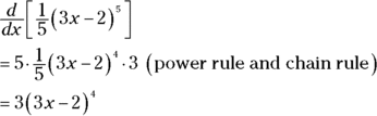
-
Tweak your first guess.
Your result,
 , is three times too much, so make your second guess a third of your first guess — that’s
  , or
, or  .
. - Check your second guess by differentiating it.
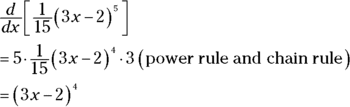
This checks. You’re done. The antiderivative of
 is
is 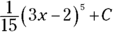
The two previous examples show that guess and check works well when the function you want to antidifferentiate has an argument like 3x or ![]() (where x is raised to the first power) instead of a plain old x. (Recall that in a function like
(where x is raised to the first power) instead of a plain old x. (Recall that in a function like ![]() , the 5x is called the argument.) In this case, you just tweak your guess by the reciprocal of the coefficient of x — the 3 in
, the 5x is called the argument.) In this case, you just tweak your guess by the reciprocal of the coefficient of x — the 3 in ![]() , for example (the 2 in
, for example (the 2 in ![]() has no effect on your answer). In fact, for these easy problems, you don’t really have to guess and check. You can immediately see how to tweak your guess. It becomes sort of a one-step process. If the function’s argument is more complicated than
has no effect on your answer). In fact, for these easy problems, you don’t really have to guess and check. You can immediately see how to tweak your guess. It becomes sort of a one-step process. If the function’s argument is more complicated than ![]() — like the
— like the ![]() in
in ![]() — you have to try the next method, substitution.
— you have to try the next method, substitution.
Substitution
In the previous section, you can see why the first guess in each case didn’t work. When you differentiate the guess, the chain rule produces an extra constant: 2 in the first example, 3 in the second. You then tweak the guesses with 1/2 and 1/3 to compensate for the extra constant.
Now say you want the antiderivative of ![]() and you guess that it is
and you guess that it is ![]() . Watch what happens when you differentiate
. Watch what happens when you differentiate ![]() to check it.
to check it.
Here the chain rule produces an extra 2x — because the derivative of ![]() is 2x — but if you try to compensate for this by attaching a
is 2x — but if you try to compensate for this by attaching a ![]() to your guess, it won’t work. Try it.
to your guess, it won’t work. Try it.
So, guessing and checking doesn’t work for antidifferentiating ![]() — actually no method works for this simple-looking integrand (not all functions have antiderivatives) — but your attempt at differentiation here reveals a new class of functions that you can antidifferentiate. Because the derivative of
— actually no method works for this simple-looking integrand (not all functions have antiderivatives) — but your attempt at differentiation here reveals a new class of functions that you can antidifferentiate. Because the derivative of ![]() is
is ![]() , the antiderivative of
, the antiderivative of ![]() must be
must be ![]() . This function,
. This function, ![]() , is the type of function you antidifferentiate with the substitution method.
, is the type of function you antidifferentiate with the substitution method.
The substitution method works when the integrand contains a function and the derivative of the function’s argument — in other words, when it contains that extra thing produced by the chain rule — or something just like it except for a constant. And the integrand must not contain anything else.
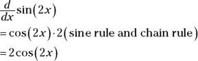
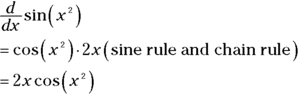
The derivative of ![]() is
is ![]() by the
by the ![]() rule and the chain rule. So, the antiderivative of
rule and the chain rule. So, the antiderivative of ![]() is
is ![]() . And if you were asked to find the antiderivative of
. And if you were asked to find the antiderivative of ![]() , you would know that the substitution method would work because this expression contains
, you would know that the substitution method would work because this expression contains ![]() , which is the derivative of the argument of
, which is the derivative of the argument of ![]() , namely
, namely ![]() .
.
You may be wondering why this is called the substitution method. I show you why in a minute. But first, I want to point out that you don’t always have to use the step-by-step method. Assuming you understand why the antiderivative of ![]() is
is ![]() , you may encounter problems where you can just see the antiderivative without doing any work. But whether or not you can just see the answers to problems like this one, the substitution method is a good one to learn because, for one thing, it has many uses in calculus and other areas of mathematics, and for another, your teacher may require that you know it and use it. So here’s how to find the antiderivative of
, you may encounter problems where you can just see the antiderivative without doing any work. But whether or not you can just see the answers to problems like this one, the substitution method is a good one to learn because, for one thing, it has many uses in calculus and other areas of mathematics, and for another, your teacher may require that you know it and use it. So here’s how to find the antiderivative of ![]() with substitution.
with substitution.
-
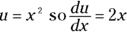
Set u equal to the argument of the main function.
The argument of
 is
is  , so you set u equal to
  .
. - Take the derivative of u with respect to x.
- Solve for dx.
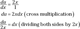
-
Make the substitutions.
In
 , u takes the place of
  and
and  takes the place of dx. So now you’ve got
  . The two 2xs cancel, giving you
  .
. - Antidifferentiate using the simple reverse rule.
-
Substitute
 back in for u — coming full circle.
u equals
 , so
, so  goes in for the u:
That’s it. So
 .
.
If the original problem had been ![]() instead of
instead of ![]() , you follow the same steps except that in Step 4, after making the substitution, you arrive at
, you follow the same steps except that in Step 4, after making the substitution, you arrive at ![]() . The xs still cancel — that’s the important thing — but after canceling you get
. The xs still cancel — that’s the important thing — but after canceling you get ![]() , which has that extra
, which has that extra ![]() in it. No worries. Just pull the
in it. No worries. Just pull the ![]() through the
through the ![]() giving you
giving you ![]() . Now you finish this problem just as you did above in Steps 5 and 6, except for the extra
. Now you finish this problem just as you did above in Steps 5 and 6, except for the extra ![]() .
.

Because C is any old constant, ![]() is still any old constant, so you can get rid of the
is still any old constant, so you can get rid of the ![]() in front of the C. That may seem somewhat unmathematical, but it’s right. Thus, your final answer is
in front of the C. That may seem somewhat unmathematical, but it’s right. Thus, your final answer is ![]() . You should check this by differentiating it.
. You should check this by differentiating it.
Here are a few examples of antiderivatives you can do with the substitution method so you can learn how to spot them.
-
The derivative of
 is
is  , but you don’t have to pay any attention to the 3 in
  or the 4 in the integrand. Because the integrand contains
  , and because it doesn’t contain any other extra stuff, substitution works. Try it.
 -

The integrand contains a function,
 , as well as the derivative of its argument, tan x — which is
  . Because the integrand doesn’t contain any other extra stuff (except for the 10, which doesn’t matter), substitution works. Do it.
 -

Because the integrand contains the derivative of sin x, namely cos x, and no other stuff except for the 2/3, substitution works. Go for it.
You can do the three problems just listed with a method that combines substitution and guess and check (as long as your teacher doesn’t insist that you show the six-step substitution solution). Try using this combo method to antidifferentiate the first example, ![]() . First confirm that the integral fits the pattern for substitution — it does, as seen in the first checklist item. This confirmation is the only part substitution plays in the combo method. Now finish the problem with guess and check.
. First confirm that the integral fits the pattern for substitution — it does, as seen in the first checklist item. This confirmation is the only part substitution plays in the combo method. Now finish the problem with guess and check.
-
Make your guess.
The antiderivative of cosine is sine, so a good guess for the antiderivative of
 is
is  .
. - Check your guess by differentiating it.

-
Tweak your guess.
Your result from Step 2,
 , is 3/4 of what you want,
  , so make your guess 4/3 bigger (note that 4/3 is the reciprocal of 3/4). Your second guess is thus
  .
. -
Check this second guess by differentiating it.
Oh, heck, skip this — your answer’s got to work.