Three functions with one limit

Consider the function in Figure 2-1. When we say that the limit of as x approaches 2 is 5, written as , we mean that as x gets closer and closer to 2 from the left and the right, gets closer and closer to a height of 5. (As far as I know, the number 2 in this example doesn’t have a formal name, but I call it the x-number.) Look at Table 2-1.

In Table 2-1, y is approaching 5 as x approaches 2 from both the left and the right, and thus the limit is 5. But why all the fuss with the numbers in the table? Why not just plug the number 2 into and obtain the answer of 5? In fact, if all functions were continuous (without gaps) as in Figure 2-1, you could just plug in the x-number to get the answer, and limit problems would basically be pointless.

We need limits in calculus because of functions like the ones in Figure 2-1 that have holes. g is identical to f except for the hole at (2, 5) and the point at (2, 3). h is identical to f except for the hole at (2, 5).

Imagine what the table of input and output values would look like for g and h. Can you see that the values would be identical to the values in Table 2-1 for f? For both g and h, as x gets closer and closer to 2 from the left and the right, y gets closer and closer to a height of 5. For all three functions, the limit as x approaches 2 is 5.

This brings us to a critical point: When determining the limit of a function as x approaches, say, 2, the value of the function when is totally irrelevant. Consider the three functions where : equals 5, is 3, and doesn’t exist (is undefined). But, again, those three results are irrelevant and don’t affect the answer to the limit problem.

In a limit problem, x gets closer and closer to the x-number but technically never gets there, and what happens to the function when x equals the x-number has no effect on the answer to the limit problem (though for continuous functions like f the function value equals the limit answer and it can thus be used to compute the limit answer).

One-sided limits

One-sided limits work like regular, two-sided limits except that x approaches the x-number from just the left or just the right. To indicate a one-sided limit, you put a superscript subtraction sign on the x-number when x approaches the x-number from the left or a superscript addition sign when x approaches it from the right:

Look at Figure 2-2. The answer to the regular limit problem, , is that the limit does not exist because as x approaches 3 from the left and the right, is not zeroing in on the same height.

However, both one-sided limits do exist. As x approaches 3 from the left, p zeros in on a height of 6, and when x approaches 3 from the right, p zeros in on a height of 2. As with regular limits, the value of has no effect on the answer to either of these one-sided limit problems. Thus,

Limits and vertical asymptotes

A rational function like has vertical asymptotes at and . Remember asymptotes? They’re imaginary lines that a function gets closer and closer to as it goes up, down, left, or right toward infinity. f is shown in Figure 2-3.

Consider the limit of f as x approaches 3. As x approaches 3 from the left, f goes up to infinity; and as x approaches 3 from the right, f goes down to negative infinity. Sometimes it’s informative to indicate this by writing,

But it’s also correct to say that both of the above limits do not exist because infinity is not a real number. And if you’re asked to determine the regular, two-sided limit, , you have to say that it does not exist because the limits from the left and from the right are unequal.

Limits and horizontal asymptotes

Up till now, I’ve been looking at limits where x approaches a regular, finite number. But x can also approach infinity or negative infinity. Limits at infinity exist when a function has a horizontal asymptote. For example, the function in Figure 2-3 has a horizontal asymptote at , which the function crawls along as it goes toward infinity to the right and negative infinity to the left. (Going left, the function crosses the horizontal asymptote at and then gradually comes down toward the asymptote.) The limits equal the height of the horizontal asymptote and are written as

Instantaneous speed

Say you decide to drop a ball out of your second-story window. Here’s the formula that tells you how far the ball has dropped after a given number of seconds (ignoring air resistance):

(where h is the height the ball has fallen, in feet, and t is the amount of time since the ball was dropped, in seconds)

If you plug 1 into t, h is 16; so the ball falls 16 feet during the first second. During the first 2 seconds, it falls a total of , or 64 feet, and so on. Now, what if you wanted to determine the ball’s speed exactly 1 second after you dropped it? You can start by whipping out this trusty ol’ formula:

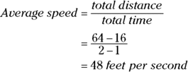
Using the rate, or speed formula, you can easily figure out the ball’s average speed during the 2nd second of its fall. Because it dropped 16 feet after 1 second and a total of 64 feet after 2 seconds, it fell , or 48 feet from second to seconds. The following formula gives you the average speed:

But this isn’t the answer you want because the ball falls faster and faster as it drops, and you want to know its speed exactly 1 second after you drop it. The ball speeds up between 1 and 2 seconds, so this average speed of 48 feet per second during the 2nd second is certain to be faster than the ball’s instantaneous speed at the end of the 1st second. For a better approximation, calculate the average speed between second and seconds. After 1.5 seconds, the ball has fallen , or 36 feet, so from to , it falls , or 20 feet. Its average speed is thus

If you continue this process for elapsed times of a quarter of a second, a tenth, a hundredth, and so on, you arrive at average speeds shown in Table 2-2.

As t gets closer and closer to 1 second, the average speeds appear to get closer and closer to 32 feet per second.

Here’s the formula I used to generate the numbers in Table 2-2. It gives you the average speed between 1 second and t seconds. Figure 2-4 shows the graph of this function.

This graph is identical to the graph of the line except for the hole at (1, 32). There’s a hole there because if you plug 1 into t in the average speed function, you get

which is undefined. And why did you get ? Because you’re trying to determine an average speed — which equals total distance divided by elapsed time — from to . But from to is, of course, no time, and “during” this point in time, the ball doesn’t travel any distance, so you get as the average speed from to .

Obviously, there’s a problem here. Hold on to your hat — you’ve arrived at one of the big “Ah ha!” moments in the development of differential calculus.

Instantaneous speed is defined as the limit of the average speed as the elapsed time approaches zero.

The fact that the elapsed time never gets to zero doesn’t affect the precision of the answer to this limit problem — the answer is exactly 32 feet per second, the height of the hole in Figure 2-4. Remarkably, limits let you calculate precise, instantaneous speed at a single point in time by taking the limit of a function that’s based on an elapsed time, a period between two points of time.

The hole exception

The hole exception is the only exception to the rule that continuity and limits go hand in hand, but it’s a huge exception. And, I have to admit, it’s a bit odd for me to say that continuity and limits usually go hand in hand and to talk about this exception because the exception is the whole point. When you come right down to it, the exception is more important than the rule. Consider the two functions in Figure 2-6.

These functions have gaps at and are obviously not continuous there, but they do have limits as x approaches 2. In each case, the limit equals the height of the hole.

An infinitesimal hole in a function is the only place a function can have a limit where it is not continuous.

So both functions in Figure 2-6 have the same limit as x approaches 2; the limit is 4, and the facts that and that is undefined are irrelevant. For both functions, as x zeroes in on 2 from either side, the height of the function zeroes in on the height of the hole — that’s the limit.

The limit at a hole is the height of the hole.

In the earlier “Instantaneous speed” section, I tried to calculate the average speed during zero elapsed time and got . Because is undefined, the result was a hole in the function. Function holes often come about from the impossibility of dividing zero by zero. It’s these functions where the limit process is critical, and such functions are at the heart of the meaning of a derivative, and derivatives are at the heart of differential calculus.

A derivative always involves the undefined fraction and always involves the limit of a function with a hole. (All the limits in Chapter 4 — where the derivative is formally defined — are limits of functions with holes.)