Chapter 8. Chemical Reactivity
Reactive chemical hazards have resulted in many accidents in industrial operations and laboratories. Preventing reactive chemical accidents requires the following steps, which are discussed in this chapter:
1. Background understanding. This includes case histories and important definitions. Case histories provide an understanding of the consequences, frequency, and breadth of reactive chemical accidents. Definitions provide a common fundamental basis for understanding. This is presented in Section 8-1 and supplemented with Chapter 14, “Case Histories.”
2. Commitment, awareness, and identification of reactive chemical hazards. This is achieved through proper management and the application of several methods to identify reactive chemical hazards. This is discussed in Section 8-2.
3. Characterization of reactive chemical hazards. A calorimeter is typically used to acquire reaction data, and a fundamental model is used to estimate important parameters to characterize the reaction. This is described in Section 8-3.
4. Control of reactive chemical hazards. This includes application of inherent, passive, active, and procedural design principles. This is discussed in Section 8-4 and supplemented by additional material in Chapters 9, “Introduction to Reliefs”; 10, “Relief Sizing”; and 13, “Safety Procedures and Designs.”
8-1. Background Understanding
In October 2002, the U.S. Chemical Safety and Hazard Investigation Board (CSB) issued a report on reactive chemical hazards.1 They analyzed 167 serious accidents in the U.S. involving reactive chemicals from January 1980 through June 2001. Forty-eight of these accidents resulted in a total of 108 fatalities. These accidents resulted in an average of five fatalities per year. They concluded that reactive chemical incidents are a significant safety problem. They recommended that awareness of chemical reactive hazards be improved for both chemical companies and other companies that use chemicals. They also suggested that additional resources be provided so that that these hazards can be identified and controlled.
On December 19, 2007, an explosion occurred at T2 Laboratories in Jacksonville, Florida. Four people were killed and 32 injured due to the explosion. The facility was producing a chemical product to be used as a gasoline octane additive. The explosion was caused by the bursting of a large reactor vessel due to a runaway reaction. A runaway reaction occurs when the process is unable to remove adequate heat from the reactor to control the temperature. The reactor temperature subsequently increases, resulting in a higher reaction rate and an even faster rate of heat generation. Large commercial reactors can achieve heating rates of several hundred degrees Celsius per minute during a runaway.
The CSB investigated the T2 Laboratories accident and found that the company engineers did not recognize the runaway hazards associated with this chemistry and process and were unable to provide adequate controls and safeguards to prevent the accident. They found that, even though the engineers were degreed chemical engineers, they did not have any instruction on reactive hazards. The CSB recommended adding reactive hazard awareness to chemical engineering curriculum requirements.
A chemical reactivity hazard is “a situation with the potential for an uncontrolled chemical reaction that can result directly or indirectly in serious harm to people, property or the environment.”2 The resulting reaction may be very violent, releasing large quantities of heat and possibly large quantities of toxic, corrosive, or flammable gases or solids. If this reaction is confined in a container, the pressure within the container may increase very quickly, eventually exceeding the pressure capability of the container, resulting in an explosion. The reaction may occur with a single chemical, called a self-reacting chemical (e.g., monomer), or with another chemical, called either a chemical interaction or incompatibility.
Note that the hazard is due to the potential for a chemical reaction. Something else must occur for this hazard to result in an accident. However, as long as reactive chemicals are stored and used in a facility, the reactive chemical hazard is always present.
One of the difficulties with reactive chemicals hazards is that they are difficult to predict and identify. Common materials that we use routinely by themselves with negligible hazard may react violently when mixed with other common materials, or react violently when the temperature or pressure is changed.
Chemical reactivity occurs in chemical plants due to the following scenarios:
1. Chemicals reacting by design, for example, in your process reactor, to produce a desired product.
2. Chemicals reacting by accident, for example, due to an upset in the process, loss of containment, etc.
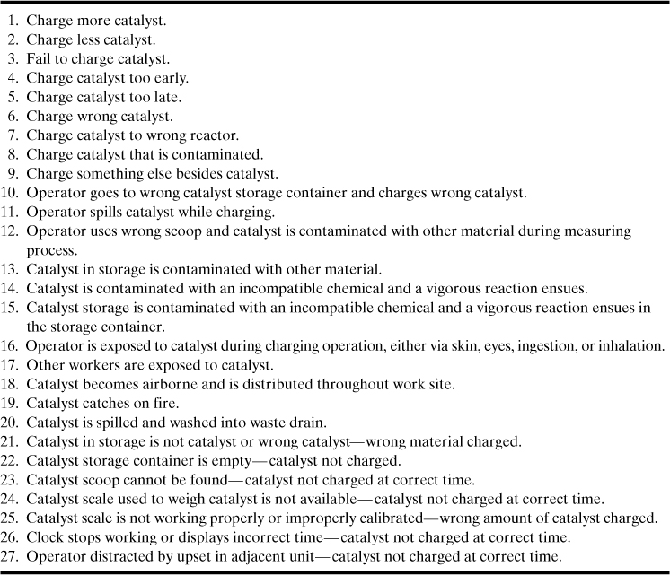
Human factors are also important in reactive chemical incidents. Suppose an operator is given the task to “Charge 10 kg of catalyst to reactor B at 3:00 pm” Table 8-1 lists some of the ways in which this operator may fail to perform this task properly. As can be seen, many failure modes are possible, and this is only one instruction in a sequence of possibly hundreds of steps.
Table 8-1. Possible Failure Modes for the Single Instruction “Charge 10 kg of Catalyst to Reactor B at 3:00 PM”
8-2. Commitment, Awareness, and Identification of Reactive Chemical Hazards
The first step in this process is to commit to manage reactive chemical hazards properly. This requires commitment from all employees, especially management, to properly identify and manage these hazards throughout the entire life cycle of a process. This includes laboratory research and development; pilot plant studies; and plant design, construction, operation, maintenance, expansion, and decommissioning.
Figure 8-1 is a flowchart useful for preliminary screening for reactive chemicals hazards. Figure 8-1 contains seven questions to help identify reactive chemical hazards.
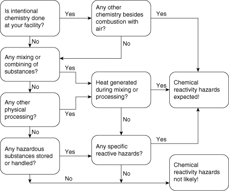
Figure 8-1. Screening flowchart for reactive chemical hazards. An answer of “yes” at any decision point moves more toward reactive chemisty. See Section 8.2 for more details. Source: R. W. Johnson, S.W. Rudy, and S. D. Unwin, Essential Practices for Managing Chemical Reactivity Hazards (New York: AIChE Center for Chemical Process Safety, 2003.)
1. Is intentional chemistry performed at your facility? In most cases this is easy to determine. The bottom line is: Are the products that come out of your facility in a different molecular configuration from the raw materials? A precise answer to this question is required prior to moving forward in the flowchart.
2. Is there any mixing or combining of different substances? If substances are mixed or combined, or even dissolved in a liquid or water, then it is possible that a reaction, either intended or unintended, may occur.
3. Does any other physical processing of substances occur in your facility? This could include size reduction, heating/drying, absorption, distillation, screening, storage, warehousing, repackaging, and shipping and receiving.
4. Are there any hazardous substances stored or handled at your facility? The Materials Safety Data Sheet (MSDS) is a good source of information here.
5. Is combustion with air the only chemistry intended at your facility? This includes combustion of common fuels such as natural gas, propane, fuel oil, etc. Combustion is a special reactive hazard that is handled by separate codes and standards and is not addressed here.
6. Is any heat generated during the mixing, phase separation, or physical processing of substances? Heat generation when chemicals are mixed is a prime indication that a reaction is taking place. Note that many chemicals do not release much heat during the reaction, so even if limited heat is released, a chemical reaction may still be occurring. There are also some physical heat effects, such as absorption or mechanical mixing, that can cause heat generation. This heat release, even though not caused by chemical reaction, may increase the temperature and cause a chemical reaction to occur.
7. Are there any specific reaction hazards that occur? Specific reaction hazards are shown in Table 8-2 with detailed lists of chemical categories and chemicals provided in Appendix F. Functional groups that are typically associated with reactive chemistry are shown in Table 8-3.
Table 8-2. Specific Reactive Chemical Hazardsa
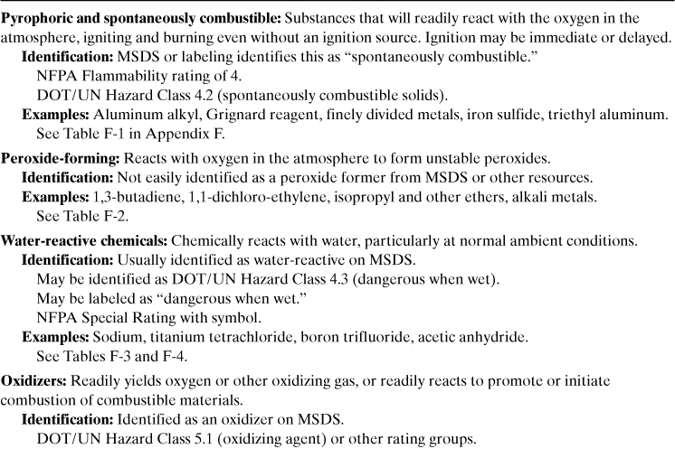
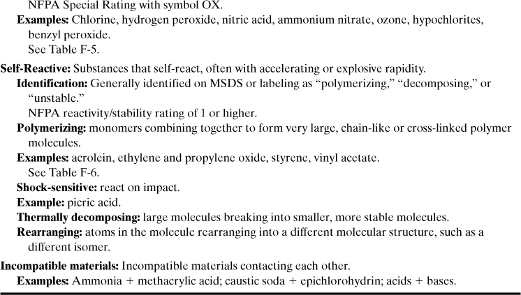
a See Johnson et al., Essential Practices for Managing Chemical Reactivity Hazards, for additional detail on these classifications, as well as Appendix F for more detailed lists of these materials.
Table 8-3. Reactive Functional Groupsa
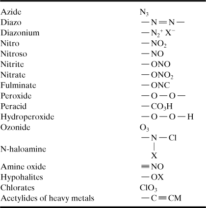
a Conrad Schuerch, “Safe Practice in the Chemistry Laboratory: A Safety Manual,” in Safety in the Chemical Laboratory, v. 3, Norman V. Steere, ed. (Easton, PA: Division of Chemical Education, American Chemical Society, 1974), pp. 22–25.
One of the most difficult reactive chemical hazards to characterize is incompatible chemicals, shown at the bottom of Table 8-2. Common materials that we use routinely and safely by themselves may become highly reactive when mixed. These materials may react very quickly, possibly producing large amounts of heat and gas. The gas may be toxic or flammable.
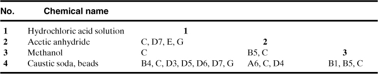
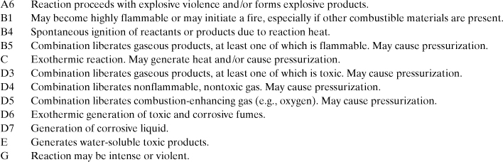
The easiest way to show graphically the various interactions between chemicals is a chemical compatibility matrix, as shown in Table 8-4. The chemicals are listed on the left-hand side of the table. The chemicals selected may be all of the chemicals in a facility, or the chemicals that may come in contact with each other during routine or emergency situations. Clearly, listing all the chemicals provides a conservative result, but may result in a large and unwieldy matrix.
Table 8-4. Chemical Compatibility Matrix and Hazards for Example 8-1, as Predicted by CRW 2.02
Individual Chemical Hazards and Functional Groups
Each table entry in the chemical compatibility matrix shows the interaction between two chemicals in the table. Thus, the table entry just to the right of acetic anhydride represents the binary interaction between acetic anhydride and hydrochloric acid solution.
The chemical compatibility matrix only considers binary interactions between two chemicals. Binary interactions would be expected during routine operations, while combinations of several chemicals may occur during emergency situations. However, once the hazards are identified using the binary interactions of all chemicals, additional hazards due to combinations of more than two chemicals are unlikely.
Once the chemicals are identified, the binary interactions are filled in. Information for these interactions can be obtained from a variety of sources, as shown in Table 8-5. Perhaps the easiest source to use is the Chemical Reactivity Worksheet (CRW).3 This worksheet is provided free of charge by the Office of Emergency Management of the U.S. Environmental Protection Agency, the Emergency Response Division of the National Oceanic and Atmospheric Administration (NOAA), and the AIChE Center for Chemical Process Safety. The software contains a library of 5000 common chemicals and mixtures and considers 43 different organic and inorganic reactive groups. CRW also provides information on the hazards associated with specific chemicals and also the reactive group(s) associated with those chemicals, as shown at the bottom of Table 8-4. CRW tends to be conservative on its predictions of binary interactions so the results must be carefully interpreted.
Table 8-5. Sources of Information on Chemical Reactivity Hazards
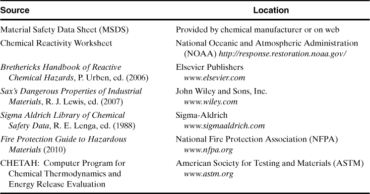
Another source of information on reactive chemicals is a program called CHETAH. CHETAH stands for Chemical Thermodynamics and Energy Release Evaluation. This program is able to predict the reactive chemical hazards using functional groups. CHETAH was originally developed by Dow Chemical and is very useful as an initial screening tool for reactive chemical hazards.
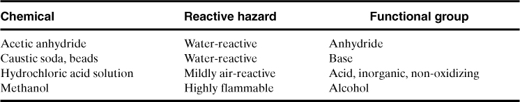
A laboratory contains the following chemicals: hydrochloric acid solution, acetic anhydride, methanol, and caustic soda (NaOH) beads. Draw a chemical compatibility matrix for these chemicals. What are the major hazards associated with these chemicals?
The chemicals are entered into the Chemical Reactivity Worksheet (CRW) software and the chemical compatibility matrix is shown in Table 8-4. Table 8-4 also lists the major hazard and reactive group associated with each chemical.
From Table 8-4 it is clear that the mixing of any of these chemicals will result in a hazardous situation! All of these chemicals must be stored separately, and management systems must be enforced to ensure that accidental mixing does not occur.
Since each combination in the matrix contains the letter C, it is clear that an exothermic reaction is expected with the mixing of any pair of chemicals. Three combinations (hydrochloric acid + caustic soda; acetic anhydride + methanol; methanol + caustic soda) liberate a gaseous product, at least one of which is flammable. Two combinations (hydrochloric acid + acetic anhydride; hydrochloric acid + caustic soda) result in an intense or violent reaction. One combination (acetic anhydride + caustic soda) results in a reaction with explosive violence and/or forms explosive products. Other hazards are listed in Table 8-4.
From the individual hazards table at the bottom of Table 8-4, two of the chemicals (acetic anhydride and caustic soda) are water-reactive, one chemical (hydrochloric acid solution) is mildly air-reactive, and methanol is flammable. The prediction of air reactivity with the hydrochloric acid solution is probably a bit conservative.
All personnel using these chemicals in the laboratory must be aware of both the individual chemical hazards and the reactive hazards that result when these chemicals are mixed.
8-3. Characterization of Reactive Chemical Hazards Using Calorimeters
Chemical plants produce products using a variety of complex reactive chemistries. It is essential that the behavior of these reactions be well characterized prior to using these chemicals in large commercial reactors. Calorimeter analysis is important to understand both the desired reactions and also undesired reactions.
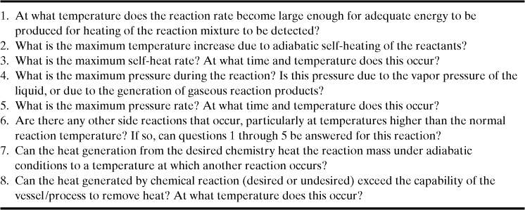
Some of the important questions that must be asked in order to characterize reactive chemicals are shown in Table 8-6. The answers to these questions are necessary to design control systems to remove heat from the reaction to prevent a runaway; to design safety systems, such as a reactor relief, to protect the reactor from the effects of high pressure (see Chapters 9 and 10); and to understand the rate at which these processes occur. The answers must be provided at conditions as close as possible to actual process conditions.
Table 8-6. Important Questions for the Characterization of Reactive Chemicals
For exothermic reactions, heat is lost through the walls of the reactor vessel to the surroundings. The higher these heat losses, the lower the temperature inside the reactor. Conversely, the lower the heat losses, the higher the temperature within the reactor. We can thus conclude that we will reach the highest reaction temperatures and highest self-heating rates when the reactor has no heat losses, that is, adiabatic.
The heat losses through the walls of the reactor are proportional to the surface area of the reactor vessel. As the vessel becomes larger, the surface-to-volume ratio becomes smaller and the heat losses through the walls have a smaller effect. Thus, as the vessel becomes larger, the behavior of the vessel approaches adiabatic behavior.
Many chemical plant personnel believe that a large reactor will self-heat at a rate that is a lot slower than a much smaller vessel. In reality the reverse is true: A larger reactor vessel will approach adiabatic conditions and the self-heat rates will be a lot faster.
As discussed above, heat removal rates do not scale linearly with increased reactor volume. This scaling problem has been the cause of many incidents. Reactions tested in the laboratory or pilot plant frequently showed slow self-heat rates that were controlled easily using ice baths or small cooling coils. However, when these reactions were scaled up to large commercial reactors, sometimes having volumes of 20,000 gallons or more, the self-heat rates were sometimes orders of magnitude higher, resulting in an uncontrollable temperature increase and explosion of the reaction vessel. Large commercial reactors with energetic chemicals such as acrylic acid, ethylene or propylene oxide, and many others can achieve self-heat rates as high as hundreds of degrees Celsius per minute!
Introduction to Reactive Hazards Calorimetry
The idea behind the calorimeter is to safely use small quantities of material in the laboratory to answer the questions shown in Table 8-6. Most of the calorimeters discussed in this chapter have test volumes from a few ml to as high as 150 ml. Larger test volumes more closely match industrial reactors but also increase the hazards associated with the laboratory test.
The calorimeter technology presented here was developed mostly in the 1970s. Much of the early development was done by Dow Chemical4,5,6 although numerous researchers have made significant contributions since then.
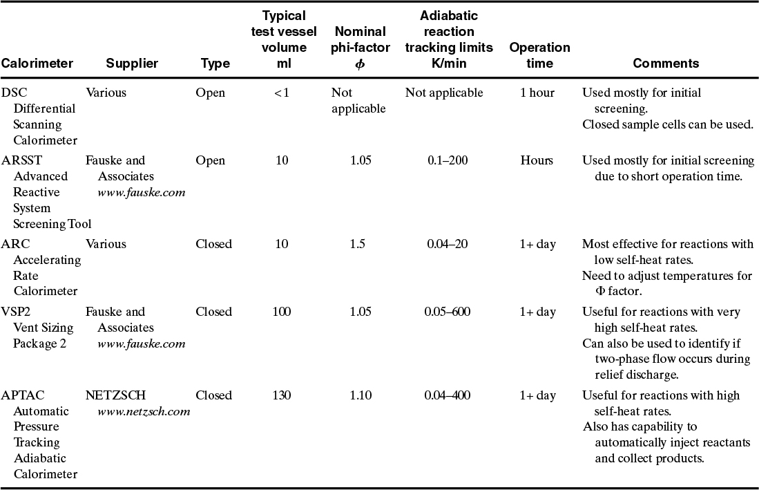
Table 8-7 summarizes the commonly used calorimeters that are available for reactive chemicals testing. All of the calorimeters hold the sample in a small sample cell. All of the calorimeters have a means to heat the test sample and measure the temperature of the sample as a function of time. Most also have the capability to measure the pressure inside the closed sample cell.
Table 8-7. Types of Calorimeters Most Commonly Used to Study Reactive Chemicals
It is important that the calorimeter be as close as experimentally possible to adiabatic behavior in order to ensure that the results are representative of a large reactor. The adiabatic conditions will also ensure the “worst-case” results, i.e.: highest temperature and pressure and highest self-heat rates and pressure rates.
All of the calorimeters have two modes of operation. The most common mode, called the thermal scan mode, is to heat the sample at a constant temperature rate (for example, 2°C per minute) until the reaction rate becomes large enough for adequate energy to be produced for the calorimeter to detect the reaction heating. This is called the thermal scan mode. Two of the calorimeters in Table 8-7—DSC and Advanced Reactive System Screening Tool (ARSST)—continue to heat beyond this temperature. All of the other calorimeters stop the heating once the reaction heating is detected and then switched to an adiabatic state by matching the outside temperature to the sample temperature.
The other mode of heating is to heat the sample up to a fixed temperature and then wait for a specified time to see if any reaction self-heating is detected. If self-heating is detected, the calorimeter is placed immediately in adiabatic mode. If no self-heating is detected after a specific time, the temperature is again incremented and the process is repeated. This is called the heat-wait-search mode.
Several calorimeters—the Accelerating Rate Calorimeter (ARC), Vent Sizing Package (VSP2), and Automatic Pressure Tracking Adiabatic Calorimeter (APTAC)—have the capability to do both heating modes during the same run.
The thermal scan mode is most often used for reactive chemicals studies. The heat-wait-search mode is used for chemicals that have a long induction time, meaning they take a long time to react.
In adiabatic mode, the calorimeter attempts to adjust the heaters outside the sample cell to match the temperature inside the sample cell. This ensures that there is no heat flow from the sample cell to the surroundings, resulting in adiabatic behavior.
The calorimeters are classified as either open or closed. An open calorimeter is one in which the sample cell is either open to the atmosphere or open to a large containment vessel. Two calorimeters in Table 8-7—the DSC and ARSST—are classified as open. For the traditional DSC, the sample cell is completely open to the atmosphere, and no pressure data are collected. Some DSCs have been modified to use sealed capillary tubes or sealed high-pressure metal holders. For the ARSST, the small sample cell (10 ml) is open to a much larger (350 ml) containment vessel. A pressure gauge is attached to the containment vessel, but only qualitative pressure data are collected from this gauge. The ARSST containment vessel is also pressurized with nitrogen during most runs to prevent the liquid sample from boiling so that higher reaction temperatures can be reached.
Since the ARC is a closed system, this calorimeter can also be used to determine the vapor pressure of the liquid mixture. This is done by first evacuating the ARC and then adding the test sample. The pressure measured by the ARC is then the vapor pressure; this can be measured as a function of temperature.
It is fairly easy to insulate a small sample cell to approach near adiabatic conditions. However, the sample cell must be capable of withstanding reaction pressures that may be as high as hundreds of atmospheres. The easiest approach to achieve high-pressure capability is to use a thick-walled vessel capable of withstanding the pressure. The problem with this is that the thick walls of the sample cell will absorb heat from the test sample, resulting in less than adiabatic conditions. The presence of a vessel that absorbs heat increases the thermal inertia of the test device and reduces both the maximum temperature and also the maximum temperature rate.
The thermal inertia of the apparatus is represented by a phi-factor, defined by
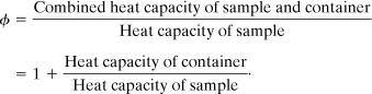
Clearly, a phi-factor as close as possible to 1 represents less thermal inertia. Most large commercial reactors have a phi-factor of about 1.1.
Table 8-7 lists the phi-factors for the most common calorimeters. The ARC uses a thick-walled vessel to contain the reaction pressure; it has a high phi-factor as a result. The ARSST uses a thin-walled glass sample cell that is open to the containment vessel. Since this glass vessel contains only the test sample and does not need to withstand the pressure developed by the reaction, it has a low phi-factor.
The VSP2 and the APTAC use a unique control method to reduce the phi-factor. Both of these calorimeters use thin-walled containers to reduce the heat capacity of the sample cell. Figure 8-2 shows a schematic of the VSP2 calorimeter. The sample is contained in a closed, thin-walled test cell, which is held in a containment vessel. The control system measures the pressure inside the test cell and also the pressure inside the containment vessel. The control system is able to rapidly adjust the pressure inside the containment vessel to match the pressure inside the test cell. The pressure difference between the inside of the test cell and the containment device is kept as low as possible, usually less than 20 psi. As a result, the thin-walled sample cell does not rupture.
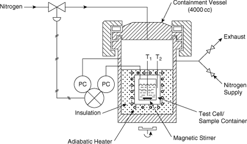
Figure 8-2. Vent Sizing Package (VSP2) showing the control system to equalize the pressure between the sample cell and the containment vessel.
The adiabatic reaction tracking limits shown in Table 8-7 relate to the lower rate at which the self-heating is detected and the upper reaction rate that the calorimeter can follow.
The operation time in Table 8-7 is an approximate idea of how long it takes to do a single, standard run on the apparatus. Some of the calorimeters (DSC and ARSST) have short run times; these calorimeters are useful for doing numerous screening studies to get an initial idea of the reactive nature of the material before moving to a more capable, but longer operation time, calorimeter.
The Differential Scanning Calorimeter (DSC) consists of two small sample cells, one containing the unknown sample and the other containing a reference material. The two samples are heated and the DSC measures the difference in heat required to maintain the two samples at the same temperature during this heating. This apparatus can be used to determine the heat capacity of the unknown sample, the temperature at which a phase change occurs, the heat required for the phase change, and also the heat changes due to a reaction. For a traditional DSC the trays are open to the atmosphere, so this type of calorimeter is classified as an open type, as shown in Table 8-7. The DSC can also be modified to use sealed glass capillary tubes or small metal containers. The DSC is mostly used for quick screening studies to identify if a reactive hazard is present and to get an initial idea of the temperatures at which the reaction occurs. The traditional DSC does not provide any pressure information since the pans are open. If sealed glass capillary tubes are used, limited pressure information can be obtained from the pressure at which the tube ruptures.
Figures 8-3 and 8-4 show typical temperature and pressure scans for an APTAC device. In Figure 8-3 the sample is heated at a constant temperature rate until an exotherm is detected as shown. The calorimeter then switches to adiabatic mode. In adiabatic mode, the calorimeter measures the temperature of the sample and attempts to match the external temperature to the sample temperature. This ensures near-adiabatic behavior. During adiabatic mode, the sample self-heats by the energy released by the reaction. Eventually, the reactants are all consumed and the reaction terminates. Self-heating stops at this point and the temperature remains constant. At the end of the run, the calorimeter heating is turned off and the sample cools.
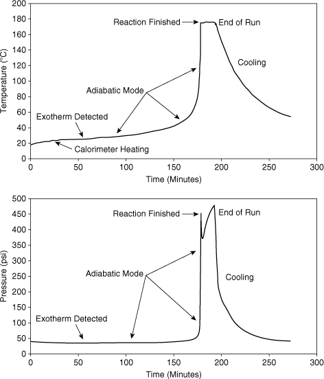
Figure 8-3. APTAC data for the reaction of methanol and acetic anhydride.
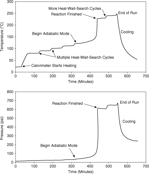
Figure 8-4. APTAC data for the thermal decomposition of di-tert-butyl peroxide.
The plot at the bottom of Figure 8-3 shows the pressure scan for this APTAC run. The pressure increase is due to the vapor pressure of the liquid sample. This pressure increases exponentially with temperature. The decrease and then increase in pressure after the reaction is finished would merit additional study—it might be due to the decomposition of one of the reaction products.
Figure 8-4 shows a calorimeter run using the heat-wait-search mode. The sample is incrementally heated using a user-defined temperature step, and then the calorimeter waits for a specified time, looking for any reaction heating. Several heat-wait-search cycles are required before an exotherm is detected and the calorimeter goes into adiabatic mode. At the completion of the reaction, the calorimeter goes back into the heat-wait-search mode, looking for additional reactions at higher temperatures.
Another mode of calorimeter operation is to inject a chemical at a specified temperature. It is also possible to heat the calorimeter with chemical A in the sample container, and then inject chemical B at a specified temperature. Both of these methods will result in an injection endotherm as the cold liquid is injected, but the calorimeter will quickly recover.
The calorimeter selected for a particular study depends on the nature of the reactive material. Many companies do screening studies using the DSC or ARSST and then, depending on the screening results, move to a more capable calorimeter. If a very slow reaction is expected, then the ARC has the best ability to detect very low heating rates. If the reaction has a very high self-heat rate, then the VSP2 or APTAC is the calorimeter of choice.
Theoretical Analysis of Calorimeter Data
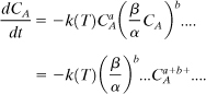
Assume that we have a reaction occurring in a closed, well-stirred reaction test cell. Assume a general reaction of the form
We can then write a mole balance on reactant A as follows:
where
C is the concentration (moles/volume),
k(T) is the temperature-dependent rate coefficient (concentration1–n/time), and
a, b ... are the reaction orders with respect to each species.
The rate coefficient k(T) is given by the Arrhenius equation Ae–Ea/RgT, where A is the pre-exponential factor and Ea is the activation energy.
Equation 8-3 can be written for each species for the reaction shown in Equation 8-2.
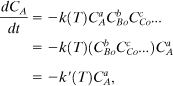
If the reactants are initially added to the reaction test cell in their stoichiometric ratios, then the concentrations will remain at those ratios throughout the reaction. Then
and similarly for all of the other species. Substituting into Equation 8-3,
We can then write an equation for the concentration of species A in terms of an overall reaction order n = a + b + ... and define a new rate coefficient k′. Then
This approach only works if all of the species are stoichiometric.
Another approach is to have all the reactants, except one, be in excess. In this case the excess reactant concentrations can be assumed to be approximately constant during the reaction. Suppose that all the reactants, except species A, are in excess. Then
where CBo is the initial concentration of species B. This approach is useful for determining the reaction order with respect to an individual species.
Consider now a situation where the reaction order is not known. Assume that the reaction can be represented by an overall nth-order reaction of the following form:
We can define a reaction conversion x in terms of the initial concentration Co:
Note that when C = Co, x = 0 and when C = 0, x = 1.
Substituting Equation 8-9 into Equation 8-8,
Dividing both sides of Equation 8-10 by ![]() ,
,
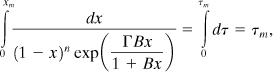
Now define a dimensionless time τ as
and Equation 8-11 simplifies to
Up to this point all our equations are cast with respect to the concentration within our reaction vessel. Unfortunately, the concentration is very difficult to measure, particularly when the reaction is very fast and the concentrations are changing very rapidly. On-line instruments to measure the concentration directly are still very limited. A more direct approach would be to withdraw a very small sample from the reactor and cool and quench the reaction instantaneously to get a representative result. Withdrawing the sample would also have an impact on the test sample since we are removing mass and energy from the vessel. Thus, measuring the concentration in real time is very difficult to do.
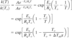
The easiest system parameter to measure is the temperature. This can be done easily with a thermocouple and can be done very rapidly in real time. We can relate the temperature to the conversion by assuming that the conversion is proportional to the entire temperature change during the reaction. This gives us the following equation:
where
To is the initial reaction temperature, also called the reaction onset temperature,
TF is the final reaction temperature when the reaction is completed, and
ΔTad is the adiabatic temperature change during the reaction.
Equation 8-14 contains two important assumptions. These are
1. The reaction is characterized by an initial and final temperature, and these temperatures can be determined experimentally with a fair amount of precision.
2. The heat capacity of the test sample is constant during the reaction.
Assumption 1 is perhaps the more important. The initial or onset temperature must be the temperature at which the reaction rate becomes large enough for adequate energy to be produced for heating of the reaction mixture to be detected by a thermocouple. This temperature has been misinterpreted by many investigators in the past. Some investigators have incorrectly concluded that if a reactive material is stored below the initial or onset temperature, then that reactive mixture will not react. This is totally incorrect, since the reaction proceeds at a finite, albeit often undetectable rate, even below the onset temperature. Different calorimeters will also give different initial or onset temperatures since this is a function of the temperature measurement sensitivity of the calorimeter. The initial or onset temperature is used only to relate the concentration of the reactant to the temperature of the reactor, and nothing more.
Assumption 2 will fail if the heat capacity of the products is significantly different from the heat capacity of the reactants. Fortunately, the heat capacities for most liquid materials are about the same. If the reactants are mostly liquids and a significant fraction of the products are gases, then this assumption may fail. This assumption is approximately true if one or more of the reactants are in excess or the system contains a solvent in high concentration, resulting in a nearly constant liquid heat capacity.
The kinetic term in Equation 8-13 can be expanded as follows:

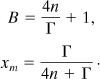
Now define B as the dimensionless adiabatic temperature rise and Γ as the dimensionless activation energy, given by the following equations:
Then Equation 8-13 reduces to the following dimensionless equation:
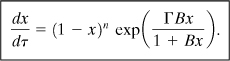
If the dimensionless adiabatic temperature rise B, is small, that is, less than about 0.4, then Equation 8-19 simplifies to
Equations 8-19 and 8-20 contain the following very important assumptions:
1. The reaction vessel is well mixed. This means that the temperature and concentration gradients in the liquid sample are small.
2. The physical properties—heat capacity and heat of reaction—of the sample are constant.
3. The heat released by the reaction is proportional to the conversion.
4. The reaction conversion x is directly proportional to the temperature increase during the reaction.
By converting our dimensional equations into dimensionless form we reduce the equations to their simplest form, thus allowing easy algebraic manipulation of the equations. We also identify the least number of dimensionless parameters required to describe our system. In this case there are three parameters: reaction order n, dimensionless adiabatic temperature rise B, and dimensionless activation energy Γ. Finally, the equations are easier to solve numerically since all variables are scaled, typically between 0 and 1.
The problem with using a dimensionless approach is that the dimensionless parameters and variables are difficult to interpret physically. Also, some effort might be required to convert from dimensional variables to dimensionless variables.
The reaction order, n, has typical values between 0 and 2. The reaction order is almost always greater than 1 and fractional orders are likely. The dimensionless adiabatic temperature rise, B, has typical values from 0 to about 2. The dimensionless activation energy, Γ, can have values ranging from about 5 to 50 or higher depending on the activation energy.
Our dimensionless Equations 8-19 and 8-20 depend on a number of dimensional parameters. These includes onset temperature To, final temperature TF, activation energy Ea, and the value of the Arrhenius equation at the onset temperature k(To). Note that the onset and final temperatures are implicitly related to the Arrhenius reaction rate equation and cannot be specified independently.
Equations 8-19 and 8-20 can be easily integrated. This can be done using a spreadsheet and the trapezoid rule, or a mathematical package. A spreadsheet using the trapezoid rule might require a small step size; this should be checked to ensure that the results are converged.
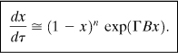
Figures 8-5 and 8-6 show the results for the integration of Equation 8-19. The conversion is plotted versus the dimensionless time. The time scale is logarithmic to show a much larger range. Figure 8-5 shows how increasing the dimensionless adiabatic temperature rise B results in a reaction that occurs over a shorter time period with a steeper slope. Figure 8-6 shows how increasing the dimensionless activation energy Γ also results in a reaction that occurs over a shorter time period and a steeper slope. For the case with Γ = 20, the conversion responds very quickly.
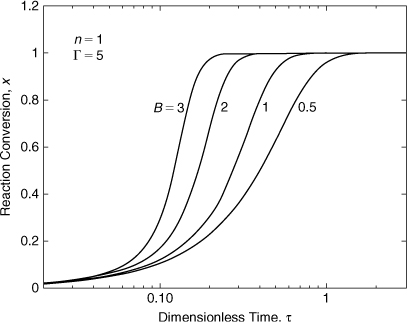
Figure 8-5. Equation 8-20 solved for increasing dimensionless adiabatic temperature rise B.
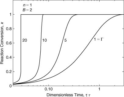
Figure 8-6. Equation 8-20 solved for increasing dimensionless activation energy Γ.
One of the important questions in Table 8-6 is the maximum self-heat rate and the time at which this occurs. The maximum self-heat rate is important for designing heat transfer equipment to remove the heat of reaction—larger self-heat rates require larger heat transfer equipment. Some chemicals, such as ethylene oxide and acrylic acid, will self-heat at rates of several hundred degrees Celsius per minute. The time at which the maximum self-heat rate occurs is also important for designing heat transfer equipment as well as for emergency response procedures.
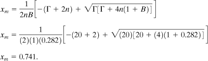
The maximum self-heat rate can be found by differentiating Equation 8-19 with respect to the dimensionless time τ and then setting the result to zero to find the maximum. This equation can be solved for the conversion xm at which the maximum self-heat rate occurs. After a lot of algebra, the following equation is obtained:
where xm is the conversion at the maximum rate. The maximum rate is then found by substituting xm into Equation 8-19.
Figure 8-7 is a plot of Equation 8-21 for a first-order reaction. As Γ increases, an asymptotic function is approached. This function is close to the Γ = 64 curve shown. Also, there is a maximum xm for each curve. The maximum xm increases as Γ increases and also occurs at lower B values. Each curve intersects the x axis.
Figure 8-7. Conversion at maximum self-heat rate for a first-order reaction. The vertical line on each curve represents the maximum value.
Equation 8-21 can be differentiated one more time with respect to B to find the maximum value of xm. After a fair amount of algebra, the maximum value is found to occur at
The intersection of the curves on Figure 8-7 with the x axis means that the maximum selfheat rate occurs at the onset temperature, that is, when τ = 0. The value of B at this intersection can be found from Equation 8-21 by setting xm = 0 and solving for B. The result is
The time to the maximum self-heat rate is found by separating variables in Equation 8-19 and integrating. The result is
where τm is the dimensionless time at which the maximum rate occurs. Note that this time is relative to the onset temperature.
Equation 8-24 can be solved numerically for τm. The results are shown in Figures 8-8 and 8-9 for two different ranges of Γ. Each curve has a maximum, shown by the vertical tick mark. This maximum occurs at lower Γ values as the dimensionless adiabatic temperature rise B increases. This maximum must be solved for numerically—an algebraic solution is not possible.
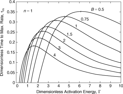
Figure 8-8. Time to maximum self-heat rate for a first-order reaction—low Γ range. The vertical lines on each curve represent the maximum value.
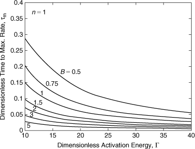
Figure 8-9. Time to maximum self-heat rate for a first-order reaction—high Γ range.
A chemical reactor currently has a temperature of 400 K. Given the calorimetry data provided below, calculate:
a. The current conversion.
b. The current self-heat rate.
c. The time since the onset temperature.
d. The time to the maximum self-heat rate.
e. The maximum self-heat rate.
Calorimeter data:
From the calorimetry data provided:
a. The current conversion is found from Equation 8-14:
b. The current self-heat rate is calculated using Equation 8-19:
This must be converted to dimensional time. From Equation 8-12,
and using the definition of the conversion given by Equation 8-14:
And it follows for n = 1,
The dimensionless time since the onset temperature is found by integrating Equation 8-19. This can be done easily using either a spreadsheet or a numerical package. The results are shown in Figure 8-10. From Figure 8-10, at a conversion of 0.217 the dimensionless time is 0.141. The dimensionless time can be converted to actual time using Equation 8-25. For a first-order reaction, n = 1 and
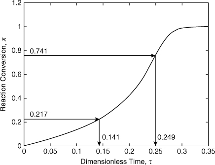
Figure 8-10. Conversion plot for Example 8-2.
This is the time since the onset temperature.
c. The conversion at the maximum rate is given by Equation 8-21. Substituting the known values:
From the numerical solution, Figure 8-10, the dimensionless time at this conversion is 0.249. The actual time is
This is with respect to the time the onset temperature is reached. The time from the current reaction state (x = 0.217) to the time at the maximum rate is
73.9 min – 41.8 min = 32.1 min
Thus, the reaction will reach the maximum rate in 32.1 min.
Figure 8-8 or 8-9 could be used to solve this problem directly. However, it is not as precise.
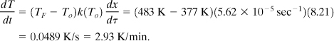
d. The maximum self-heat rate is found using Equation 8-19:
It follows that
The maximum self-heat rate, along with the heat capacity of the reacting liquid, could be used to estimate the minimum cooling requirements for this reactor. Also, the time to maximum rate could be used to estimate the residence time, operating temperature, and conversion for the reactor.
Estimation of Parameters from Calorimeter Data
Prior to using the theoretical model, we need to estimate from calorimeter data the parameters required for the model. These include onset temperature To, final temperature TF, reaction order n, activation energy Ea, and the value of the Arrhenius equation at the onset temperature k(To). The calorimeter typically provides temperature versus time data so a procedure is required to estimate these parameters from these data.
The onset and final temperatures are perhaps the most important since the conversion, and the theoretical model, depends on knowing these parameters reasonably precisely. If we plot the rate of temperature change dT/dt versus time, we find that the temperature rate is very low at the beginning and end of the reaction. Thus, this procedure will not work.
A better procedure is to plot the logarithm of the rate of temperature change dT/dt versus –1000/T. This is best illustrated by an example.
Figure 8-3 shows temperature time and pressure time data for the reaction of methanol and acetic anhydride in a 2:1 molar ratio. Using these data, estimate the onset and final temperatures and the dimensionless adiabatic temperature rise B for this system.
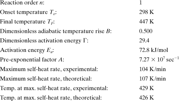
A plot of the logarithm of the temperature rate versus –1000/T is shown in Figure 8-11. The temperature rates at early times are shown on the left-hand side of the plot and the temperature rates at the end of the experiment are on the right. When the calorimeter detects exothermic behavior, it stops the heating. This is shown as a drop in the plotted temperature rate on the far left side of Figure 8-11. The onset temperature is found as the temperature at the beginning of the nearly straight-line section of the curve. The onset temperature from Figure 8-10 is found to be 298 K.
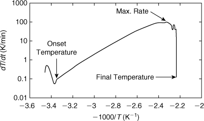
Figure 8-11. Graphical procedure to estimate the onset and final temperatures.
The final temperature is found from the right-hand side of the plot where the temperature rate drops off suddenly and returns to almost the same temperature rate as the onset temperature. The final temperature identified from Figure 8-11 is 447 K.
Figure 8-11 can also be used to identify the maximum temperature rate as well as the temperature at which this occurs. This is found from the peak value in Figure 8-11. From the data, the maximum temperature rate is 104 K/min (1.73 K/sec), and this occurs at a temperature of 429 K.
The dimensionless adiabatic temperature rise is given by Equation 8-17. Thus,
At this point in the procedure we have the onset and final temperatures and the dimensionless adiabatic temperature rise B.
The next parameter to estimate is the reaction order. The reaction order can be estimated by rearranging Equation 8-19 as follows:
From Equation 8-12, ![]() , and it follows that
, and it follows that
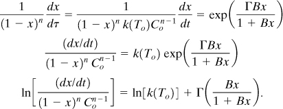
Equation 8-28 can be modified in terms of the actual temperature. Since dx = dT/(TF – To),
For a first-order reaction, n = 1, and (1 – x) = (TF – T)/(TF – To), and Equation 8-29 can be simplified even further:
The procedure for determining the overall reaction order n, using either Equation 8-28, Equation 8-29, or 8-30 is as follows. The onset and final temperatures, and the dimensionless adiabatic temperature rise B, are already known from Example 8-3. First, the overall reaction order is guessed. First-order (n = 1) is a good place to start. The conversion x can be calculated from the temperature data using Equation 8-14. Then the left-hand side of either Equation 8-28, 8-29, or 8-30 is plotted versus Bx/(1 + Bx). If the reaction order is correct, a straight line is obtained. It is possible to have fractional overall reaction orders, so some effort might be required to estimate the reaction order that produces the best fit to the data. For any reaction order not equal to unity, the initial concentration of reactant must be known. Finally, as a bonus, once the reaction order is identified, the intercept of the straight line with the y axis provides an estimate of k(To).
If we assume a first-order reaction (n = 1) and substitute to convert Equation 8-30 into dimensional form, the following equation is obtained:
Equation 8-31 states that if a system is first-order, then a plot of the left-hand side versus –1/RgT should produce a straight line with slope of Ea and intercept ln A. Equation 8-31 is commonly seen in the literature as a means to determine the kinetic parameters. It is not as general as Equation 8-28.
Using the data in Figure 8-3 and the results of Examples 8-2 and 8-3, estimate the reaction order and the value of k(To) for the methanol + acetic anhydride reaction (2:1 molar ratio). Use these parameters to estimate the pre-exponential factor A and the activation energy Ea. Use the theoretical model to calculate the maximum self-heat rate and corresponding temperature. Compare to the experimental values.
The first step in this problem is to convert the temperature data into conversion data, x. This is done using the onset and final temperatures from Example 8-3 and Equation 8-14. Then (dx/dt) is calculated using the trapezoid rule or any other suitable derivative method. Equation 8-29 is then applied with an initial assumption that n = 1. We then plot ln ![]() versus
versus ![]() . These results are shown in Figure 8-12. If we eliminate some of the early and later points in the data that diverge from the straight line—these points have less precision—and fit a straight line to the remaining data, we get a very straight line with an R2 value of 0.9997. This confirms that the reaction is first-order.
. These results are shown in Figure 8-12. If we eliminate some of the early and later points in the data that diverge from the straight line—these points have less precision—and fit a straight line to the remaining data, we get a very straight line with an R2 value of 0.9997. This confirms that the reaction is first-order.
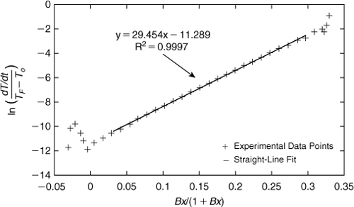
Figure 8-12. Determination of the kinetic parameters n, Γ, and k(To).
From the straight-line fit, the slope is equal to our dimensionless parameter Γ and the intercept is equal to ln k(To). Thus, Γ = 29.4 and ln k(To) = –11.3. It follows that k(To) = 1.24 × 10⁻⁵ sec–1.
From the definition for Γ given by Equation 8-18, the activation energy Ea is computed as 72.8 kJ/mol, and since k(To) = A exp (–Ea / RgTo), we can calculate the pre-exponential factor as A = 7.27 × 10⁷ sec–1.
The conversion at the maximum self-heat rate is given by Equation 8-21:
Substituting the known values,
The temperature at this conversion is
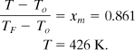
This compares very well to the experimental maximum rate temperature of 429 K.
The maximum self-heat rate is estimated from Equation 8-19, with n = 1:
The maximum self-heat rate in dimensional units is calculated from Equation 8-26:
This compares to the experimental value of 1.73 K/sec (104 K/min). The experimental maximum self-heat rate is usually lower than the theoretical value due to the dampening effect of the sample container heat capacity. Figure 8-13 is a plot of the experimental and theoretical temperature-time plots. The agreement is very good.
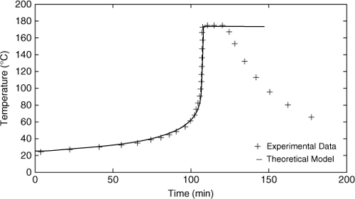
Figure 8-13. Comparison of experimental data with theoretical model prediction.
Summary of Calorimeter Analysis: Ethanol + Acetic Anhydride
Adjusting the Data for the Heat Capacity of the Sample Vessel
Up to now, the calorimeter data analysis has assumed that the sample vessel container has a negligible heat capacity. This situation is not realistic—the sample vessel always has a heat capacity that absorbs heat during the chemical reaction.
The sample container absorbs heat during the reaction and reduces the total temperature change during the reaction. Thus, without the container, the final reaction temperature would be higher.
The effect of the sample container on the temperature can be estimated from a heat balance. The goal is to estimate the change in temperature of the isolated sample, without the container. The heat generated by the isolated reacting sample is distributed between the sample and the sample container. In equation form,
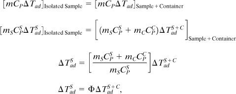
where Φ is the phi-factor presented earlier in Equation 8-1.
Equation 8-32 shows that, for example, if the reaction occurs in a reaction container with a phi-factor of 2, then the container absorbs half of the heat generated by the reaction and the measured adiabatic temperature increase is half of the temperature increase that would be measured by an isolated sample.
The theoretical model can be adjusted by replacing the dimensionless adiabatic temperature rise B by Φ B to account for the heat capacity of the container.
The initial reaction temperature is not affected much by the container presence. However, the final reaction temperature is estimated from the following equation:
Heat of Reaction Data from Calorimeter Data
Calorimeter analysis can provide additional information beyond the kinetic model analysis discussed so far.
Calorimeter data can be used to estimate the heat of reaction of the reacting sample. This is done using the following equation:
ΔHrx is the heat of reaction, energy/mass, based on the limiting reactant;
Φ is the phi-factor for the vessel container, given by Equations 8-1 and 8-33, unitless;
CV is the heat capacity at constant volume for the reacting liquid, energy/mass-deg;
ΔTad is the adiabatic temperature rise during the reaction, deg;
mLR is the initial mass of limiting reactant, mass; and
mT is the total mass of reacting mixture, mass.
Using Pressure Data from the Calorimeter
The pressure information provided by the calorimeter is very important, especially for relief system and pressure vessel design. If the calorimeter is the closed vessel type, the vessel can be evacuated prior to addition of the sample. The pressure data are then representative of the vapor pressure of the reacting liquid—important data required for relief sizing.
The pressure data are used to classify reaction systems into four different types.7 These classifications are important for relief system design, discussed in Chapter 10. The classifications are based on the dominant energy term in the liquid reaction mass as material is discharged through the relief system.
1. Volatile/tempered reaction: This is also called a vapor system. In this case the heat of vaporization of the liquid cools, or tempers, the reaction mass during the relief discharge. Tempered reactions are inherently safer since the cooling mechanism is part of the reaction mass.
2. Hybrid/tempered reaction: Non-condensable gases are produced as a result of the reaction. However, the heat of vaporization of the liquid dominates to cool the reaction mass during the entire relief discharge.
3. Hybrid/non-tempered reaction: Non-condensable gases are produced but the heat of vaporization of the liquid does not always dominate during the entire relief discharge.
4. Gassy/non-tempered reaction: The reaction produces non-condensable gases and the liquid is not volatile enough for the heat of vaporization of the liquid to have much effect during the entire relief discharge.
The pressure data from the calorimeter are used for classifying the type of system.
1. The initial and final pressure in the closed vessel calorimeter can be used to determine if the system produces a gaseous product. In this case the calorimeter must be operated so that the starting and ending temperatures are the same. If the initial pressure is equal to the final pressure, then no gaseous products are produced and the pressure is due to the constant vapor pressure of the liquid—this is a volatile/tempered reaction system. If the final pressure is higher than the starting pressure, then vapor products are produced and the reaction system is either hybrid or gassy.
2. If the system is classified as hybrid or gassy from part 1, then the time and temperature at which the peak in the temperature rate and pressure rate occurs is used. If the peaks occur at the same time and temperature, then the system is hybrid. If the peaks do not occur at the same temperature, then the system is gassy.
Application of Calorimeter Data
The calorimeter data are used to design and operate processes so that reactive chemical incidents do not occur. This is, perhaps, the most difficult part of this procedure since each process has its unique problems and challenges. Experience is essential in this procedure. Expert advice is recommended for interpreting calorimetry data and for designing controls and emergency systems.
The calorimeter data are most useful for designing relief systems to prevent high pressures due to runaway reactors. This is done using the procedures discussed in Chapter 10.
Calorimeter data are also useful for estimating or developing:
1. Heat exchanger duty to achieve required reactor cooling.
2. Cooling water requirements and cooling water pump size.
3. Condenser size in a reactor reflux system.
4. Maximum concentrations of reactants to prevent overpressure in the reactor.
5. Reactor vessel size.
6. Reactor vessel pressure rating.
7. Type of reactor: batch, semi-batch or tubular.
8. Reactor temperature control and sequencing.
9. Semi-batch reactor reactant feed rates.
10. Catalyst concentrations.
11. Alarm/shutdown setpoints.
12. Maximum fill factor for batch and semi-batch reactors.
13. Solvent concentrations required to control reactor temperature.
14. Operating procedures.
15. Emergency procedures.
16. Reactant storage vessel design and storage temperature.
17. Relief effluent treatment systems.
8-4. Controlling Reactive Hazards
If the flowchart shown in Figure 8-1 and discussed in section 8-1 shows that reactive hazards are present in your plant or operation, then the methods shown in Table 8-8 are useful to control these hazards and prevent reactive chemicals incidents. Table 8-8 is only a partial list of methods—many more methods are available. The methods are classified as inherent, passive, active or procedural. The methods at the top of the list are preferred since inherent and passive methods are always preferred over active and procedural methods.
Table 8-8. Hierarchy of methods to improve reactive chemicals safety. This is only a partial list of possibilities.
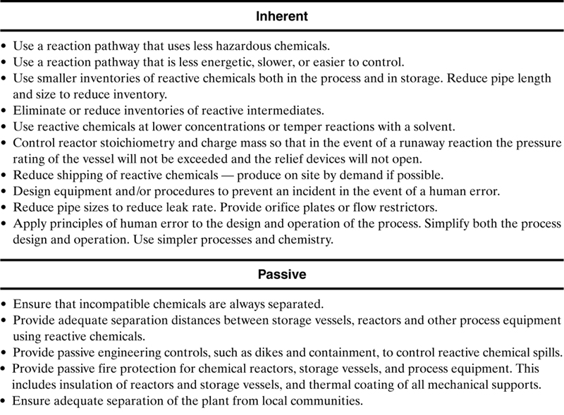
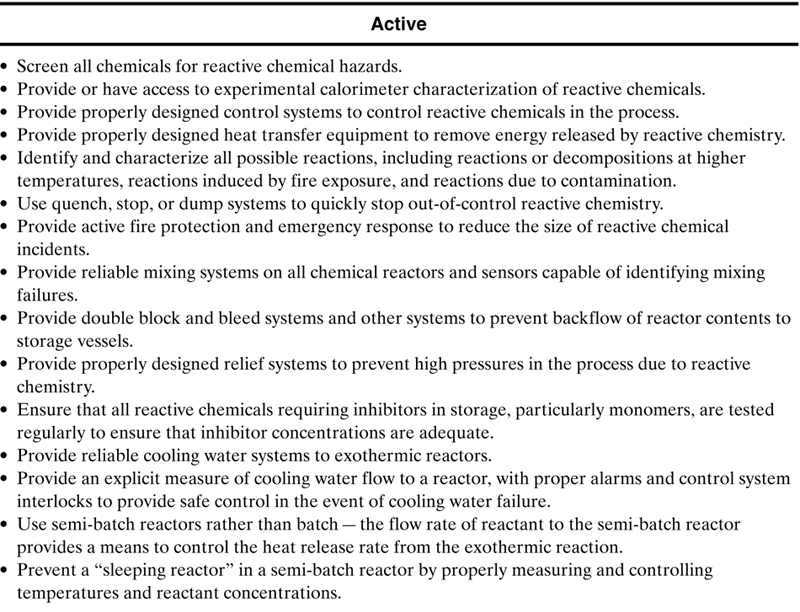
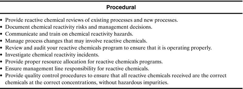
The procedural methods in Table 8-8, even though they are low on the hierarchy, are essential for any effective reactive chemicals management system. These are discussed in detail in Johnson, et al.8
A chemical reactive hazards program requires a considerable amount of technology, experience, and management to prevent incidents in any facility handling reactive chemicals. This requires awareness and commitment from all employees, from upper management on down, and the resources necessary to make it all work.
Suggested Reading
Center for Chemical Process Safety (CCPS), Guidelines for Safe Storage and Handling of Reactive Chemicals (New York: American Institute of Chemical Engineers, 1995).
H. G. Fisher, H. S. Forrest, S. S. Grossel, J. E. Huff, A. R. Muller, J. A. Noronha, D. A. Shaw, and B. J. Tilley, Emergency Relief System Design Using DIERS Technology (New York: AIChE Design Institute for Emergency Relief Systems, 1992).
R. W. Johnson, “Chemical Reactivity,” pp. 23–24 to 23–30, Perry’s Chemical Engineers’ Handbook, 8th ed., D. W. Green, ed. (New York: McGraw-Hill, 2008).
D. C. Hendershot, “A Checklist for Inherently Safer Chemical Reaction Process Design and Operation,” International Symposium on Risk, Reliability and Security (New York: American Institute of Chemical Engineers Center for Chemical Process Safety, 2002).
Improving Reactive Hazard Management (Washington, DC: US Chemical Safety and Hazard Investigation Board, October 2002).
L. E. Johnson and J. K. Farr, “CRW 2.0: A Representative-Compound Approach to Functionality-Based Prediction of Reactive Chemical Hazards,” Process Safety Progress (2008), 27(3): 212–218.
R. W. Johnson, S. W. Rudy, and S. D. Unwin, Essential Practices for Managing Chemical Reactivity Hazards (New York: AIChE Center for Chemical Process Safety, 2003).
A. Kossoy and Y. Akhmetshin, “Identification of Kinetic Models for the Assessment of Reeaction Hazards,” Process Safety Progress (2007), 26(3): 209.
D. L. Townsend and J. C. Tou, “Thermal Hazard Evaluation by an Accelerating Rate Calorimeter,” Thermochimica Acta (1980), 37: 1–30.
Problems
8-1. Professor Crowl’s laboratory contains the following inventory of chemicals: methanol, sodium hydroxide in solid beads, acetic anhydride, methane, hydrogen, nitrogen, and oxygen. The methane, hydrogen, nitrogen, and oxygen are contained in K-cylinders, which hold about 200 SCF of gas. Please help Professor Crowl by preparing a chemical compatibility matrix for these chemicals. Provide recommendations on what represents the greatest hazard.
8-2. A company had a spray painting operation to paint automotive parts. The spray painting was done in a paint booth to reduce workers’ exposure and to collect any paint droplets that might be entrained in the exhaust air. The paint droplets were collected by fibrous filters. At the end of each day, the filters were removed, placed in plastic bags, and stored for disposal in a separate building.
Due to environmental concerns over volatile emissions from paint solvents, the paint supplier reformulated the paint to use a less volatile solvent. This change was done in consultation with the paint company. Several tests were done to ensure that the reformulated paint worked well with the existing spray equipment and that the resulting quality was satisfactory.
The company eventually switched over to the reformulated paint. Several days later the disposal building caught on fire, apparently due to a fire started by the paint filters.
Can you explain how this happened? Any suggestions for prevention?9
8-3. A contract manufacturer is contracted to prepare one 8100 lb batch of a gold precipitating agent. Ingredients are mixed in a 125 ft3 (6 m3) cone blender which is insulated and has a steel jacket to allow cooling and heating with a water/glycol mixture. The precipitating agent consists of approximately 66% sodium hydrosulfite, 22% aluminum powder, and 11% potassium carbonate by weight. After blending these dry ingredients, a small amount of liquid benzaldehyde is added for odor control. The product blend is packaged into eighteen 55 gal drums for shipment.9
This operation is entirely a blending procedure. This same blender is also used for other formulations and has cooling capability that uses a water/ethylene glycol mixture as the cooling medium. Apply the screening method of Figure 8-1 to determine if any chemical reactivity hazards are expected.
8-4. Eastown Industries conducted a Management of Change review for switching to a new propylene dichloride supplier. The propylene dichloride was purchased in railcar quantities and unloaded into a large storage tank, from which it was metered into 55 gal drums for sale to customers. During the Management of Change review, it was identified that the supplier sometimes used aluminum railcars for other products. The shift supervisor raised the question of what would happen if the propylene dichloride was received in an aluminum railcar and remained on the siding for a few days before unloading its contents into the storage tank.9
Use the NOAA Chemical Reactivity Worksheet (CRW) as a resource to decide if the propylene dichloride is compatible with the aluminum in the tank cars.
8-5. A university lab expansion includes installation of a distribution system to provide gaseous oxygen from manifolded cylinders to a biological laboratory. No chemical reactivity hazards have been previously identified for the lab facilities.9
Apply the screening method of Figure 8-1 to determine if any chemical reactivity hazards are expected.
8-6. Redo Figures 8-5 and 8-6 for a second-order reaction using the same parameters. How does the reaction order affect the behavior?
8-7. Redo Figure 8-7 for second-order reaction. How does the reaction order affect the behavior?
8-8. Redo Figures 8-8 and 8-9 for a second-order reaction. How does the reaction order affect the behavior?
8-9. Derive Equation 8-21 by differentiating Equation 8-19 with respect to τ, solving for the maximum by setting the result to zero, and then solving for xm.
8-10. Derive Equation 8-23.
8-11. Derive Equation 8-22. Note: This is a lot of tedious algebra!
8-12. Starting from Equation 8-20, show that the maximum self-heat rate for small values of B is given by
What happens for large Γ? At xm = 0? At ΓB = n?
8-13. Derive Equation 8.31 from Equation 8-30.
8-14. A commonly used equation in calorimetry analysis to determine the temperature at the maximum rate is given by
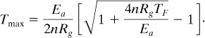
Derive this equation from Equation 8-21. Use this equation to calculate Tmax for the ethanol acetic anhydride system of Examples 8-3 and 8-4. Compare to the experimental value.
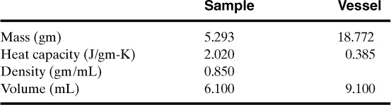
8-15. 3.60 gm of vacuum-distilled acrylic acid is placed in a titanium test vessel in an ARC.
Estimate the phi-factor for this experiment.
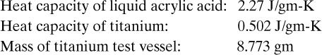
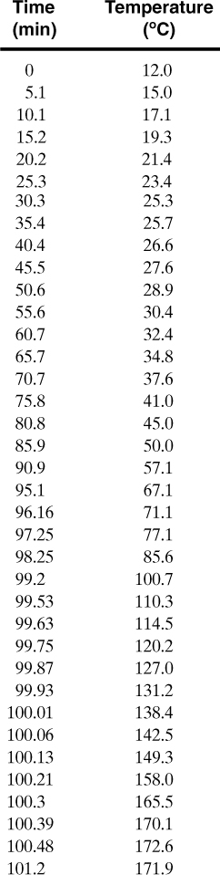
8-16. The data below are raw data from the ARSST. Assume a first-order reaction for this system. The heating rate for the calorimeter is 0.3 °C/min.
a. Plot the temperature rate versus –1000/T to estimate the onset and final temperatures.
b. Use Equation 8-32 to determine the kinetic parameters A and Ea for the original raw data.
8-17. The ARSST continues to heat the test sample during the entire exotherm. Thus, the data must be adjusted for this continuous heating. This adjustment is done by realizing that the temperature rise measured by the calorimeter, ΔTMeasured, is composed of both the adiabatic temperature increase due to the reaction, ![]() , and the temperature increase due to the calorimeter heating, ΔTExternal:
, and the temperature increase due to the calorimeter heating, ΔTExternal:
The temperature increase due to the calorimeter heating is given by
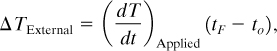
where
(dT/dt)Applied is the applied heating rate, deg/time;
tF is the time at the final temperature; and
to is the time at the onset temperature.
Use Equations 8-36 and 8-37 to adjust the temperatures of the raw data from Problem 8-16 for the imposed heating rate from the calorimeter. Repeat Problem 8-16 to determine the kinetic parameters with the adjusted data.
8-18. The phi-factor for the ARSST is about 1.05 (Table 8-7). Adjust the data from Problem 8-16 for the phi-factor and estimate the kinetic parameters.
8-19. Using the raw data from Problem 8-16, calculate A and Ea for each case shown below. How does each case affect the quantities calculated?
a. Reduce the time period over which the reaction occurs by one-half.
b. Keep the same times, but double the adiabatic temperature rise.
c. Comment on how these changes affect the results.
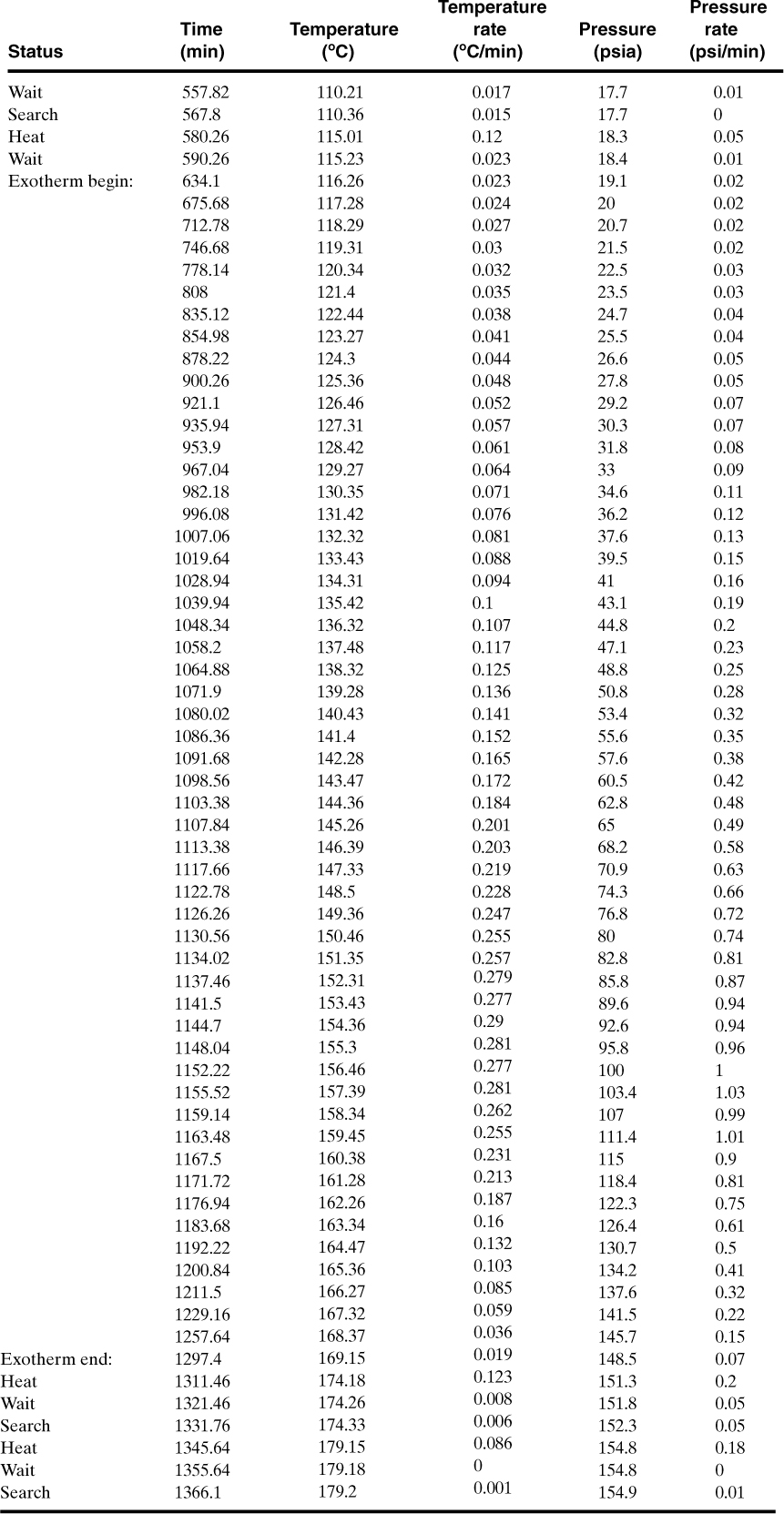
8-20. Shown below are calorimetry data for the reaction of 14.2 wt. % cumene hydroperoxide (CHP) in cumene in an ARC. The ARC is operated in a heat-wait-search mode, as shown. The exotherm is detected by the ARC and temperature range for the exotherm is shown. Determine the following parameters for this reaction: To, TF, n, B, Γ, ln k(To), A and Ea. Use the model to predict the maximum self-heat rate—compare to experimental results. Calculate the phi-factor and adjust your final results.
Experimental conditions:
Initial concentration of limiting reactant (CHP): 0.123 gm/mL
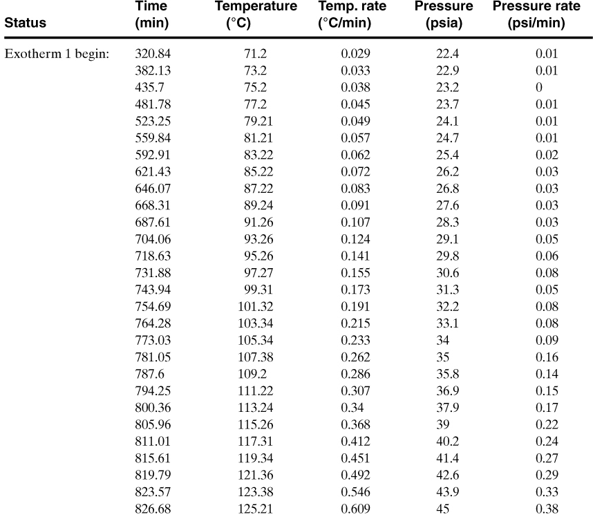
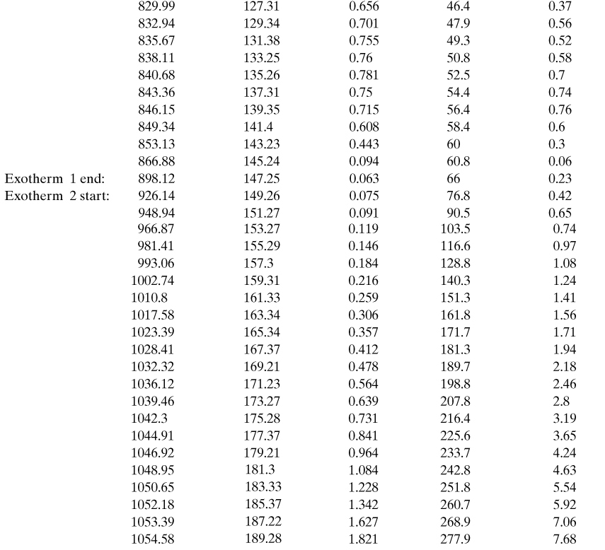
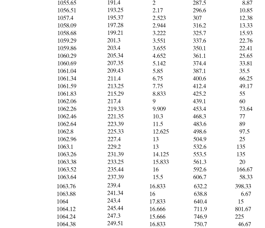
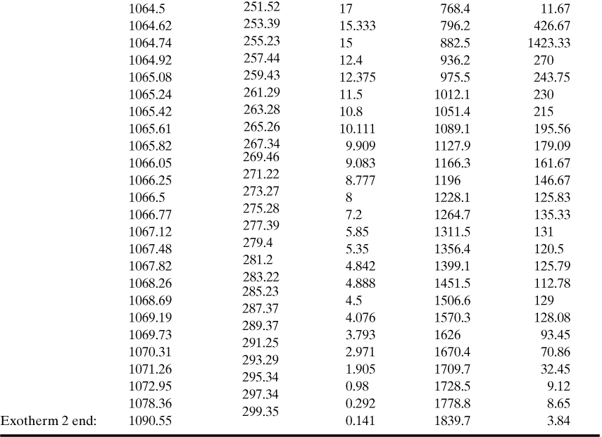
8-21. Shown below are calorimetry data from an ARC for the reaction of 50 wt. % epichlorohydrin in water. In this case there are two exotherms, one following the other. The second exotherm is most likely the decomposition of one of the products of the first reaction. Determine the following parameters for both exotherms: To, TF, B, Γ, ln k(To), A, and Ea. For the first exotherm, determine the reaction order. For the second exotherm, the initial concentration of reactant is not known; assume a first-order reaction and check if this fits the data.
Use the model to predict the maximum self-heat rate for both exotherms; compare to experimental results.
Calculate the phi-factor and adjust your final results.
Experimental conditions:
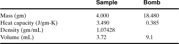
Initial concentration of limiting reactant (epichlorohydrin): 0.537 gm/mL
8-22. Your company is designing a reactor to run the methanol + acetic anhydride reaction. You have been assigned the task of designing the cooling coil system within the reactor. The reactor is designed to handle 10,000 kg of reacting mass. Assume a heat capacity for the liquid of 2.3 J/kg-K.
a. Using the results of Examples 8-3 and 8-4, estimate the heat load, in J/s, on the cooling coils at the maximum reaction rate. What additional capacity and other considerations are important to ensure that the cooling coils are sized properly to prevent a runaway reaction?
b. Using the results of part a, estimate the cooling water flow required, in kg/s. The cooling water is available at 30 °C with a maximum temperature limit of 50 °C.
8-23. Your company proposes to use a 10 m3 batch reactor to react methanol + acetic anhydride in a 2:1 molar ratio. The reactor has cooling coils with a maximum cooling rate of 30 MJ/min. Since the cooling is limiting, the decision was made to operate the reactor in semi-batch mode. In this mode, the methanol is first added to the reactor, then heated to the desired temperature, and the limiting reactant, acetic anhydride, is added at a constant rate to control the heat release.
The following data are available:
Reaction: CH3OH + (CH3CO)2O → CH3COOCH3 + CH3COOH Methanol + acetic anhydride → methyl acetate + acetic acid
Specific gravity of final liquid mixture: 0.97
Heat of reaction: 67.8 kJ/mol
Additional data are also available in Examples 8-3 and 8-4.
a. The company wants to produce this product as quickly as possible. To achieve this, at what temperature should it operate the reactor?
b. Assuming a maximum reactor fill factor of 80%, calculate the total amount of methanol, in kg, initially charged to the reactor. How much acetic anhydride, in kg, will be added?
c. What is the maximum addition rate of acetic anhydride, in kg/min, to result in a reaction heat release rate equal to the cooling capacity of the cooling coils?
d. How long, in hours, will it take to do the addition?
8-24. Using the data and information from Examples 8-3 and 8-4, estimate the heat of reaction for the methanol + acetic anhydride system. Assume a constant heat capacity for the liquid of 2.3 J/gm K and a phi-factor of 1.04. This experiment was done in the APTAC, with 37.8 gm of methanol combined with 61.42 gm of acetic anhydride, and injected into a titanium bomb of 135 ml.