
In the previous chapter, we studied Artificial Neural Networks (ANNs) and how they can be used to effectively model nonlinear sample data. So far, we've discussed several machine learning techniques that can be used to model a given training set of data. In this chapter, we will explore the following topics that focus on how to select appropriate features from the sample data:
- We will study methods to evaluate or quantify how accurately a formulated model fits the supplied training data. These techniques will be useful when we have to extend or debug an existing model.
- We will also explore how we can use the
clj-mllibrary to perform this process on a given machine learning model. - Towards the end of the chapter, we will implement a working spam classifier that incorporates a model evaluation technique.
The term machine learning diagnostic is often used to describe a test that can be run to gain insight about what is and isn't working in a machine learning model. This information generated by the diagnostic can then be used to improve the performance of the given model. Generally, when designing a machine learning model, it's advisable to formulate a diagnostic for the model in parallel. Implementing a diagnostic for a given model can take around the same time as formulating the model itself, but implementing a diagnostic is a good investment of time since it would help in quickly determining what needs to be changed in the model in order to improve it. Thus, machine learning diagnostics are helpful in saving time with respect to debugging or improving a formulated learning model.
Another interesting aspect of machine learning is that without knowing the nature of the data we are trying to fit, we can make no assumption about which machine learning model we can use to fit the sample data. This axiom is known as the No Free Lunch theorem, and can be summarized as follows:
"Without prior assumptions about the nature of a learning algorithm, no learning algorithm is superior or inferior to any other (or even random guessing)."
In the previous chapters, we've talked about minimizing the error or cost function of a formulated machine learning model. It's apt for the overall error of the estimated model to be low, but a low error is generally not enough to determine how well the model fits the supplied training data. In this section, we will revisit the concepts of overfitting and underfitting.
An estimated model is said to be underfit if it exhibits a large error in prediction. Ideally, we should strive to minimize this error in the model. However, a formulated model with a low error or cost function could also indicate that the model doesn't understand the underlying relationship between the given features of the model. Rather, the model is memorizing the supplied data, and this could even result in modeling random noise. In this case, the model is said to be overfit. A general symptom of an overfit model is failure to correctly predict the output variable from unseen data. An underfit model is also said to exhibit high bias and an overfit model is said to have high variance.
Suppose we are modeling a single dependent and independent variable in our model. Ideally, the model should fit the training data while generalizing on data that hasn't yet been observed in the training data.
The variance of the dependent variables with the independent variable in an underfit model can be represented using the following plot:
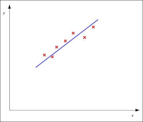
In the preceding diagram, the red crosses represent data points in our sample data. As shown in the diagram, an underfit model will exhibit a large overall error, and we must try to reduce this error by appropriately selecting the features for our model and using regularization.
On the other hand, a model could also be overfit, in which the overall error in the model has a low value, but the estimated model fails to correctly predict the dependent variable from previously unseen data. An overfit model can be depicted using the following plot:
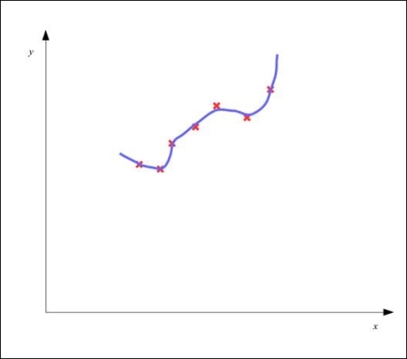
As shown in the preceding diagram, the estimated model plot closely but inappropriately fits the training data and thus has a low overall error. But, the model fails to respond correctly to new data.
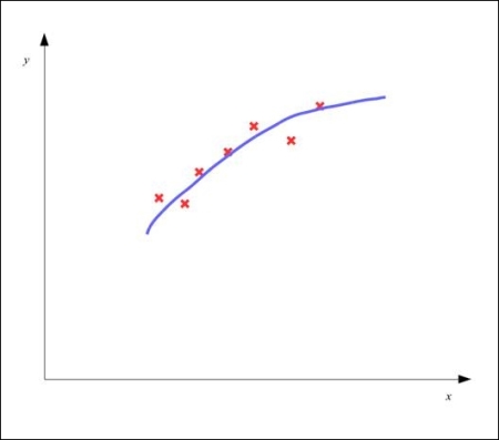
The model that describes a good fit for the sample data will have a low overall error and can predict the dependent variable correctly from previously unseen values for the independent variables in our model. An appropriately fit model should have a plot similar to the following diagram:
ANNs can also be underfit or overfit on the provided sample data. For example, an ANN with a few hidden nodes and layers could be an underfit model, while an ANN with a large number of hidden nodes and layers could exhibit overfitting.
We can plot the variance of the dependent and independent variables of a model to determine if the model is underfit or overfit. However, with a larger number of features, we need a better way to visualize how well the model generalizes the relationship of the dependent and independent variables of the model over the training data.
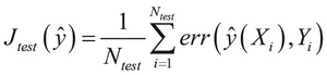
We can evaluate a trained machine learning model by determining the cost function of the model on some different data. Thus, we need to split the available sample data into two subsets—one for training the model and another for testing it. The latter subset is also called the test set of our model.
The cost function is then calculated for the ![]() samples in the test set. This gives us a measure of the overall error in the model when used on previously unseen data. This value is represented by the term
samples in the test set. This gives us a measure of the overall error in the model when used on previously unseen data. This value is represented by the term ![]() of the estimated model
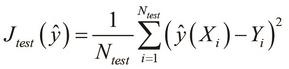
of the estimated model ![]() and is also called the test error of the formulated model. The overall error in the training data is called the training error of the model and is represented by the term
and is also called the test error of the formulated model. The overall error in the training data is called the training error of the model and is represented by the term ![]() . A linear regression model's test error can be calculated as follows:
. A linear regression model's test error can be calculated as follows:
Similarly, the test error in a binary classification model can be formally expressed as follows:
The problem of determining the features of a model such that the test error is low is termed as model selection or feature selection. Also, to avoid overfitting, we must measure how well the model generalizes over the training data. The test error on its own is an optimistic estimate of the generalization error in the model over the training data. However, we must also measure the generalization error in data that hasn't yet been seen by the model. If the model has a low error over unseen data as well, we can be certain that the model does not overfit the data. This process is termed as cross-validation.
Thus, to ensure that the model can perform well on unseen data, we will require an additional set of data, called the cross-validation set. The number of samples in the cross-validation set is represented by the term ![]() . Typically, the sample data is partitioned into the training, test, and cross-validation sets such that the number of samples in the training data are significantly greater than those in the test and cross-validate sets. The error in generalization, or rather the cross-validation error
. Typically, the sample data is partitioned into the training, test, and cross-validation sets such that the number of samples in the training data are significantly greater than those in the test and cross-validate sets. The error in generalization, or rather the cross-validation error ![]() , thus indicates how well the estimated model fits unseen data. Note that we don't modify the estimated model when we use the cross-validation and test sets on it. We will study more about cross-validation in the following sections of this chapter. As we will see later, we can also use cross-validation to determine the features of a model from some sample data.
, thus indicates how well the estimated model fits unseen data. Note that we don't modify the estimated model when we use the cross-validation and test sets on it. We will study more about cross-validation in the following sections of this chapter. As we will see later, we can also use cross-validation to determine the features of a model from some sample data.
For example, suppose we have 100 samples in our training data. We partition this sample data into three sets. The first 60 samples will be used to estimate a model that fits the data appropriately. Out of the 40 remaining samples, 20 will be used to cross-validate the estimated model, and the other 20 will be used to finally test the cross-validated model.
In the context of classification, a good representation of the accuracy of a given classifier is a confusion matrix. This representation is often used to visualize the performance of a given classifier based on a supervised machine learning algorithm. Each column in this matrix represents the number of samples that belong to a particular class as predicted by the given classifier. The rows of the confusion matrix represent the actual classes of the samples. The confusion matrix is also called the contingency matrix or the error matrix of the trained classifier.
For example, say we have two classes in a given classification model. The confusion matrix of this model might look like the following:
|
Predicted class | |||
|---|---|---|---|
|
A |
B | ||
|
Actual class |
A |
45 |
15 |
|
B |
30 |
10 | |
In a confusion matrix, the predicted classes in our model are represented by vertical columns and the actual classes are represented by horizontal rows. In the preceding example of a confusion matrix, there are a total of 100 samples. Out of these, 45 samples from class A and 10 samples from class B were predicted to have the correct class. However, 15 samples of class A have been classified as class B and similarly 30 samples of class B have been predicted to have class A.
Let's consider the following confusion matrix of a different classifier that uses the same data as the previous example:
|
Predicted class | |||
|---|---|---|---|
|
A |
B | ||
|
Actual class |
A |
45 |
5 |
|
B |
0 |
50 | |
In the preceding confusion matrix, the classifier classifies all samples of class B correctly. Also, only 5 samples of class A are classified incorrectly. Thus, this classifier better understands the distinction between the two classes of data when compared to the classifier used in the previous example. In practice, we must strive to train a classifier such that it has values close to 0 for all the elements other than the diagonal elements in its confusion matrix.
As we mentioned earlier, we need to determine an appropriate set of features from the sample data on which we must base our model. We can use cross-validation to determine which set of features to use from the training data, which can be explained as follows.
For each set or combination of feature variables, we determine the training and cross-validation error of a model based on the selected set of features. For example, we might want to add polynomial features derived from the independent variables of our model. We evaluate the training and cross-validation errors for each set of features depending on the highest degree of polynomial used to model the training data. We can plot the variance of these error functions over the degree of polynomial used, similar to the following diagram:
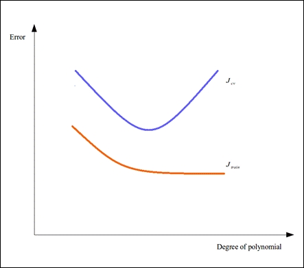
From the preceding diagram, we can determine which set of features produce an underfit or overfit estimated model. If a selected model has a high value for both the training and cross-validation errors, which is found towards the left of the plot, then the model is underfitting the supplied training data. On the other hand, a low training error and a high cross-validation error, as shown towards the right of the plot, indicates that the model is overfit. Ideally, we must select the set of features with the lowest possible values of the training and cross-validation errors.