As we mentioned earlier in Chapter 4, Building Neural Networks, SOMs can be used to model unsupervised machine learning problems such as clustering (for more information, refer to Self-organizing Maps as Substitutes for K-Means Clustering). To quickly recap, an SOM is a type of ANN that maps input values with a high number of dimensions to a low-dimensional output space. This mapping preserves patterns and topological relations between the input values. The neurons in the output space of an SOM will have higher activation values for input values that are spatially close to each other. Thus, SOMs are a good solution for clustering input data with a large number of dimensions.

The Incanter library provides a concise SOM implementation that we can use to cluster the input variables from the Iris dataset. We will demonstrate how we can use this SOM implementation for clustering in the example that will follow.

[incanter "1.5.4"]

(ns my-namespace
  (:use [incanter core som stats charts datasets]))

We first define the sample data to cluster using the get-dataset, sel, and to-matrix functions from the Incanter library as follows:

(def iris-features (to-matrix (sel (get-dataset :iris)
                                   :cols [:Sepal.Length
                                          :Sepal.Width
                                          :Petal.Length
                                          :Petal.Width])))

The iris-features variable defined in the preceding code is in fact a sized matrix that represents the values of the four input variables that we have selected from the Iris dataset. Now, we can use the som-batch-train function from the incanter.som namespace to create and train an SOM using these selected features, as follows:

(def som (som-batch-train
          iris-features :cycles 10))

The som variable defined is actually a map with several key-value pairs. The :dims key in this map contains a vector that represents the dimensions in the lattice of neurons in the trained SOM, as shown in the following code and output:

user> (:dims som)
[10.0 2.0]

Thus, we can say that the neural lattice of the trained SOM is a matrix. The :sets key of the map represented by the som variable gives us the positional grouping of the various indexes of the input values in the lattice of neurons of the SOM, as shown in the following output:

user> (:sets som)
{[4 1] (144 143 141 ... 102 100),
 [8 1] (149 148 147 ... 50),
 [9 0] (49 48 47 46 ... 0)}

As shown in the preceding REPL output, the input data is partitioned into three clusters. We can calculate the mean values of each feature using the mean function from the incanter.stats namespace as follows:

(def feature-mean
  (map #(map mean (trans
                   (sel iris-features :rows ((:sets som) %))))
       (keys (:sets som))))

We can implement a function to plot these mean values using the xy-plot, add-lines, and view functions from the Incanter library as follows:

(defn plot-means []
  (let [x (range (ncol iris-features))
        cluster-name #(str "Cluster " %)]
    (-> (xy-plot x (nth feature-mean 0)
                 :x-label "Feature"
                 :y-label "Mean value of feature"
                 :legend true
                 :series-label (cluster-name 0))
        (add-lines x (nth feature-mean 1)
                   :series-label (cluster-name 1))
        (add-lines x (nth feature-mean 2)
                   :series-label (cluster-name 2))
        view)))

The following linear plot is produced on calling the plot-means function defined in the preceding code:

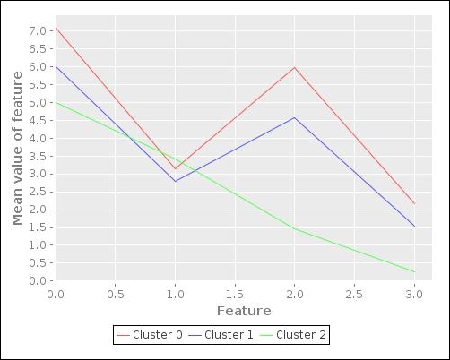
The preceding plot gives us an idea of the mean values of the various features in the three clusters determined by the SOM. The plot shows that two of the clusters (Cluster 0 and Cluster 1) have similar features. The third cluster, however, has significantly different mean values for these set of features and is thus shown as a different shape in the plot. Of course, this plot doesn't give us much information about the distribution or variance of input values around these mean values. To visualize these features, we need to somehow transform the number of dimensions of the input data to two or three dimensions, which can be easily visualized. We will discuss more on this concept of reducing the number of features in the training data in the next section of this chapter.

We can also print the clusters and the actual categories of the input values using the frequencies and sel functions as follows:

(defn print-clusters []
  (doseq [[pos rws] (:sets som)]
    (println pos :
             (frequencies
              (sel (get-dataset :iris) 
                   :cols :Species :rows rws)))))

We can call the function print-clusters defined in the preceding code to produce the following REPL output:

user> (print-clusters)
[4 1] : {virginica 23}
[8 1] : {virginica 27, versicolor 50}
[9 0] : {setosa 50}
nil

As shown in the preceding output, the virginica and setosa species seem to be appropriately classified into two clusters. However, the cluster containing the input values of the versicolor species also contains 27 samples of the virginica species. This problem could be remedied by using more sample data to train the SOM or by modeling a higher number of features.

In conclusion, the Incanter library provides us with a concise implementation of an SOM, which we can train using the Iris dataset as shown in the preceding example.