In order to easily visualize the distribution of some unlabeled data in which the input values have multiple dimensions, we must reduce the number of feature dimensions to two or three. Once we have reduced the number of dimensions of the input data to two or three dimensions, we can trivially plot the data to provide a more understandable visualization of it. This process of reducing the number of dimensions in the input data is known as dimensionality reduction. As this process reduces the total number of dimensions used to represent the sample data, it is also useful for data compression.

Principal Component Analysis (PCA) is a form of dimensionality reduction in which the input variables in the sample data are transformed into linear uncorrelated variables (for more information, refer to Principal Component Analysis). These transformed features are called the principal components of the sample data.

PCA uses a covariance matrix and a matrix operation called Singular Value Decomposition (SVD) to calculate the principal components of a given set of input values. The covariance matrix denoted as , can be determined from a set of input vectors with samples as follows:

The covariance matrix is generally calculated from the input values after mean normalization, which is simply ensuring that each feature has a zero mean value. Also, the features could be scaled before determining the covariance matrix. Next, the SVD of the covariance matrix is determined as follows:

SVD can be thought of as factorization of a matrix with size into three matrices , , and . The matrix has a size of , the matrix has a size of , and the matrix has a size of . The matrix actually represents the input vectors with dimensions in the sample data. The matrix is a diagonal matrix and is called the singular value of the matrix , and the matrices and are called the left and right singular vectors of , respectively. In the context of PCA, the matrix is termed as the reduction component and the matrix is termed as the rotation component of the sample data.

The PCA algorithm to reduce the dimensions in the input vectors to dimensions can be summarized using the following steps:

Note that the input to the PCA algorithm is the set of input vectors from the sample data after mean normalization and feature scaling.

Since the matrix calculated in the preceding steps has columns, the matrix will have a size of , which represents the input vectors in dimensions. We should note that a lower value of the number of dimensions could result in a higher loss of variance in the data. Hence, we should choose such that only a small fraction of the variance is lost.

The original input vectors can be recreated from the matrix and the reduced left singular vector as follows:

The Incanter library includes some functions to perform PCA. In the example that will follow, we will use PCA to provide a better visualization of the Iris dataset.

(ns my-namespace
  (:use [incanter core stats charts datasets]))

We first define the training data using the get-dataset, to-matrix, and sel functions, as shown in the following code:

(def iris-matrix (to-matrix (get-dataset :iris)))
(def iris-features (sel iris-matrix :cols (range 4)))
(def iris-species (sel iris-matrix :cols 4))

Similar to the previous example, we will use the first four columns of the Iris dataset as sample data for the input variables of the training data.

PCA is performed by the principal-components function from the incanter.stats namespace. This function returns a map that contains the rotation matrix and the reduction matrix from PCA, which we described earlier. We can select columns from the reduction matrix of the input data using the sel function as shown in the following code:

(def pca (principal-components iris-features))

(def U (:rotation pca))
(def U-reduced (sel U :cols (range 2)))

As shown in the preceding code, the rotation matrix of the PCA of the input data can be fetched using the :rotation keyword on the value returned by the principal-components function. We can now calculate the reduced features Z using the reduced rotation matrix and the original matrix of features represented by the iris-features variable, as shown in the following code:

(def reduced-features (mmult iris-features U-reduced))

The reduced features can then be visualized by selecting the first two columns of the reduced-features matrix and plotting them using the scatter-plot function, as shown in the following code:

(defn plot-reduced-features []
  (view (scatter-plot (sel reduced-features :cols 0)
                      (sel reduced-features :cols 1)
                      :group-by iris-species
                      :x-label "PC1"
                      :y-label "PC2")))

The following plot is generated on calling the plot-reduced-features function defined in the preceding code:

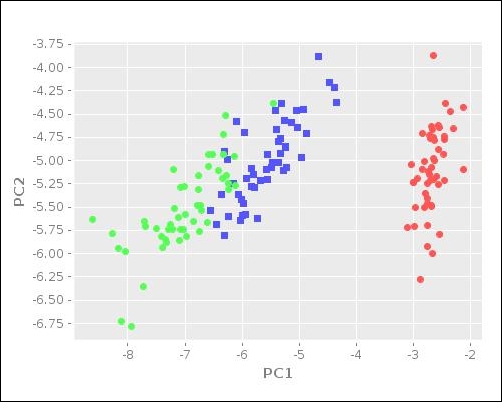
The scatter plot illustrated in the preceding diagram gives us a good visualization of the distribution of the input data. The blue and green clusters in the preceding plot are shown to have similar values for the given set of features. In summary, the Incanter library supports PCA, which allows for the easy visualization of some sample data.