We will first study some theoretical aspects about data classification. As with other supervised machine learning techniques, the goal is to estimate a model or classifier from the sample data and use it to predict a given set of outcomes. Classification can be thought of as a way of determining a function that maps the features of the sample data to a specific class. The predicted class is selected from a given set of predetermined classes. Thus, similar to regression, the problem of classifying the observed values for the given independent variables is analogous to determining a best-fit function for the given training data.

In some cases, we might be interested in only a single class, that is, whether the observed values belong to a specific class. This form of classification is termed as binary classification, and the output variable of the model can have either the value 0 or 1. Thus, we can say that , where y is the outcome or dependent variable of the classification model. The outcome is said to be negative when , and conversely, the outcome is termed positive when .

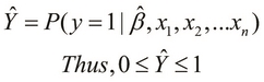
In this perspective, when some observed values for the independent variables of the model are provided, we must be able to determine the probability of a positive outcome. Thus, the estimated model of the given sample data has the probability and can be expressed as follows:

In the preceding equation, the parameters represent the independent variables of the estimated classification model , and the term represents the estimated parameter vector of this model.

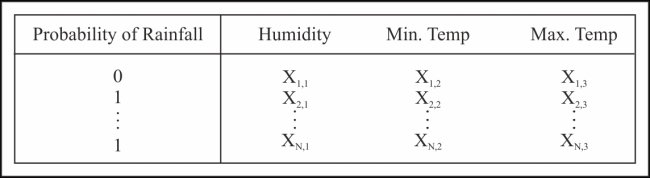
An example of this kind of classification is deciding whether a new e-mail is spam or not, depending on the sender or the content within the e-mail. Another simple example of binary classification is determining the possibility of rainfall on a particular day depending on the observed humidity and the minimum and maximum temperatures on that day. The training data for this example might appear similar to the data in the following table:

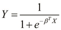
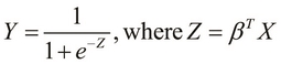
A mathematical function that we can use to model binary classification is the sigmoid or logistic function. If the outcome for the feature X has an estimated parameter vector , we can define the estimated probability of the positive outcome Y (as a sigmoid function) as follows:

To visualize the preceding equation, we can simplify it by substituting Z as as follows:

We could model the data using several other functions as well. However, the sample data for a binary classifier can be easily transformed such that it can be modeled using a sigmoid function. This modeling of a classification problem using the logistic function is called logistic regression. The simplified sigmoid function defined in the preceding equation produces the following plot:

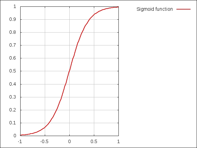
Note that if the term Z has a negative value, the plot appears reversed and is a mirror of the previous plot. We can visualize how the sigmoid function varies with respect to the term Z, through the following plot:

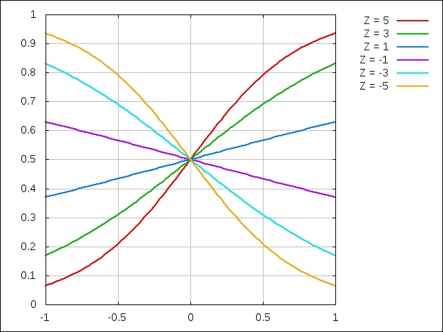
In the previous graph, the sigmoid function is shown for different values of the term ; it ranges from -5 to 5. Note that for two dimensions, the term is a linear function of the independent variable x. Interestingly, for and , the sigmoid function looks more or less like a straight line. This function reduces to a straight line when and can be represented by a constant y value (the equation in this case).

We observe that the estimated outcome Y is always between 0 and 1, as it represents the probability of a positive outcome for the given observed values. Also, this range of the outcome Y is not affected by the sign of the term . Thus, in retrospect, the sigmoid function is an effective representation of binary classification.

To use the logistic function to estimate a classification model from the training data, we can define the cost function of a logistic regression model as follows:

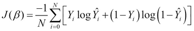
The preceding equation essentially sums up the differences between the actual and predicted values of the output variables in our model, just like linear regression. However, as we are dealing with probability values between 0 and 1, we use the preceding log function to effectively measure the differences between the actual and predicted output values. Note that the term N denotes the number of samples in the training data. We can apply the gradient descent to this cost function to determine the local minimum or rather the predicted class of a set of observed values. This equation can be regularized to produce the following cost function:

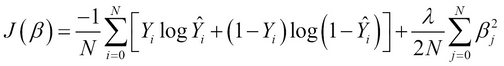
Note that in this equation, the second summation term is added as a regularization term, like we discussed in Chapter 2, Understanding Linear Regression. This term basically prevents the underfitting and overfitting of the estimated model over the sample data. Note that the term is the regularization parameter and has to be appropriately selected depending on how accurate we want the model to be.

Multiclass classification, which is the other form of classification, predicts the outcome of the classification as a value from a specific set of predetermined values. Thus, the outcome is selected from k discrete values, that is, . This model produces k probabilities for each possible class of the observed values. This brings us to the following formal definition of multiclass classification:

Thus, in multiclass classification, we predict k distinct values, in which each value indicates the probability of the input values belonging to a particular class. Interestingly, binary classification can be reasoned as a specialization of multiclass classification in which there are only two possible classes, that is, and .

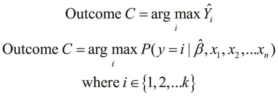
As a special case of multiclass classification, we can say that the class with the maximum probability is the outcome or simply, the predicted class of the given set of observed values. This specialization of multiclass classification is called one-vs-all classification. Here, a single class with the maximum (or minimum) probability of occurrence is determined from a given set of observed values instead of finding the probabilities of the occurrences of all the possible classes in our model. Thus, if we intend to predict a single class from a specific set of classes, we can define the outcome C as follows:

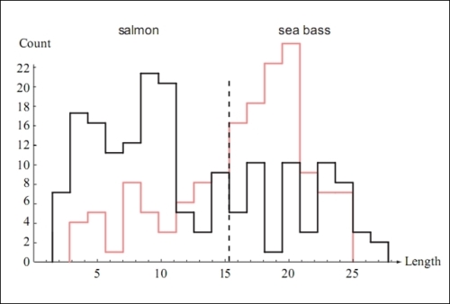
For example, let's assume that we want to determine the classification model for a fish packing plant. In this scenario, the fish are separated into two distinct classes. Let's say that we can categorize the fish either as a sea bass or salmon. We can create some training data for our model by selecting a sufficiently large sample of fish and analyzing their distributions over some selected features. Let's say that we've identified two features to categorize the data, namely, the length of the fish and the lightness of its skin.

The distribution of the first feature, that is, the length of the fish, can be visualized as follows:

Similarly, the distribution of the lightness of the skin of the fish from the sample data can be visualized through the following plot:

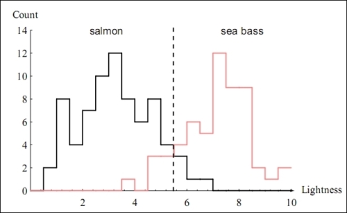
From the preceding graphs, we can say that only specifying the length of the fish is not enough information to determine its type. Thus, this feature has a smaller coefficient in the classification model. On the contrary, since the lightness of the skin of the fish plays a larger role in determining the type of the fish, this feature will have a larger coefficient in the parameter vector of the estimated classification model.

Once we have modeled a given classification problem, we can partition the training data into two (or more) sets. The surface in the vector space that partitions these two sets is called the decision boundary of the formulated classification model. All the points on one side of the decision boundary are part of one class, while the points on the other side of the decision boundary are part of the other class. An obvious corollary is that depending on the number of distinct classes, a given classification model can have several such decision boundaries.

We can now combine these two features to train our model, and this produces an estimated decision boundary between the two categories of fish. This boundary can be visualized over a scatter plot of the training data as follows:

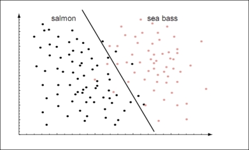
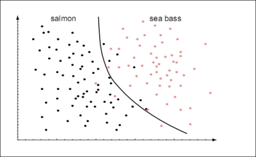
In the preceding plot, we approximate the classification model by using a straight line, and hence, we effectively model the classification as a linear function. We can alternatively model our data as a polynomial function, as it would produce a more accurate classification model. Such a model produces a decision boundary that can be visualized as follows:

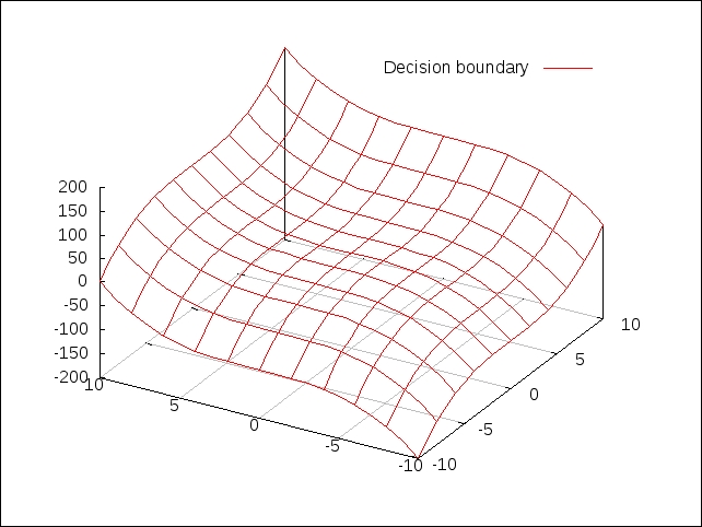
The decision boundary partitions the sample data into two dimensions as shown in the preceding graphs. The decision boundary will become more complex to visualize when the sample data has a higher number of features or dimensions. For example, for three features, the decision boundary will be a three-dimensional surface, as shown in the following plot. Note that the sample data points are not shown for the sake of clarity. Also, two of the plotted features are assumed to vary within the range , and the third feature is assumed to vary within the range .