
We will now explore the Bayesian techniques that are used to classify data. A Bayes classifier is essentially a probabilistic classifier that is built using the Bayes' theorem of conditional probability. A model based on the Bayes classification assumes that the sample data has strongly independent features. By independent, we mean that every feature of the model can vary independent of the other features in the model. In other words, the features of the model are mutually exclusive. Thus, a Bayes classifier assumes that the presence or absence of a particular feature is completely independent of the presence or absence of the other features of the classification model.
The term ![]() is used to represent the probability of occurrence of the condition or the feature A. Its value is always a fractional value within the range of 0 and 1, both inclusive. It can also be represented as a percentage valve. For example, the probability 0.5 is also written as 50% or 50 percent. Let's assume that we want to find the probability of occurrence of a feature A or
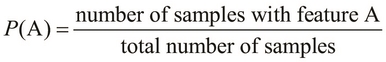
is used to represent the probability of occurrence of the condition or the feature A. Its value is always a fractional value within the range of 0 and 1, both inclusive. It can also be represented as a percentage valve. For example, the probability 0.5 is also written as 50% or 50 percent. Let's assume that we want to find the probability of occurrence of a feature A or ![]() , from a given number of samples. Thus, a higher value of
, from a given number of samples. Thus, a higher value of ![]() indicates a higher chance of occurrence of the feature A. We can formally represent the probability
indicates a higher chance of occurrence of the feature A. We can formally represent the probability ![]() as follows:
as follows:
If A and B are two conditions or features in our classification model, then we use the term ![]() to represent the occurrence of A when B is known to have occurred. This value is called the conditional probability of A given B, and the term
to represent the occurrence of A when B is known to have occurred. This value is called the conditional probability of A given B, and the term ![]() is also read as the probability of A given B. In the term
is also read as the probability of A given B. In the term ![]() , B is also called the evidence of A. In conditional probability, the two events, A and B, may or may not be independent of each other. However, if A and B are indeed independent conditions, then the probability
, B is also called the evidence of A. In conditional probability, the two events, A and B, may or may not be independent of each other. However, if A and B are indeed independent conditions, then the probability ![]() is equal to the product of the probabilities of the separate occurrences of A and B. We can express this axiom as follows:
is equal to the product of the probabilities of the separate occurrences of A and B. We can express this axiom as follows:
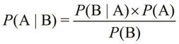
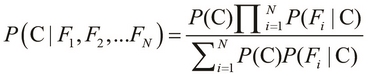
Bayes' theorem describes a relation between the conditional probabilities, ![]() and
and ![]() , and the probabilities,
, and the probabilities, ![]() and
and ![]() . It is formally expressed using the following equality:
. It is formally expressed using the following equality:
Of course, the probabilities, ![]() and
and ![]() , must both be greater than 0 for the preceding relation to be true.
, must both be greater than 0 for the preceding relation to be true.
Let's revisit the classification example of the fish packaging plant that we described earlier. The problem is that we need to determine whether a fish is a sea bass or salmon depending on its physical features. We will now implement a solution to this problem using a Bayes classifier. Then, we will use Bayes' theorem to model our data.
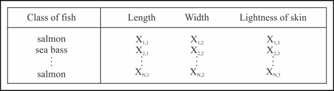
Let's assume that each category of fish has three independent and distinct features, namely, the lightness of its skin and its length and width. Hence, our training data will look like that in the following table:
For simplicity in implementation, let's use the Clojure symbols to represent these features. We need to first generate the following data:
(defn make-sea-bass []
  ;; sea bass are mostly long and light in color
  #{:sea-bass
    (if (< (rand) 0.2) :fat :thin)
    (if (< (rand) 0.7) :long :short)
    (if (< (rand) 0.8) :light :dark)})

(defn make-salmon []
  ;; salmon are mostly fat and dark
  #{:salmon
    (if (< (rand) 0.8) :fat :thin)
    (if (< (rand) 0.5) :long :short)
    (if (< (rand) 0.3) :light :dark)})

(defn make-sample-fish []
  (if (< (rand) 0.3) (make-sea-bass) (make-salmon)))

(def fish-training-data
  (for [i (range 10000)] (make-sample-fish)))
Here, we define two functions, make-sea-bass and make-salmon, to create a set of symbols to represent the two categories of fish. We conveniently use the:salmon and :sea-bass keywords to represent these two categories. Similarly, we can also use Clojure keywords to enumerate the features of a fish. In this example, the lightness of skin is either :light or :dark, the length is either :long or :short, and the width is either :fat or :thin. Also, we define the make-sample-fish function to randomly create a fish that is represented by the set of features defined earlier.
Note that we define these two categories of fish such that the sea bass are mostly long and light in skin color, and the salmon are mostly fat and dark. Also, we generate more salmon than sea bass in the make-sample-fish function. We add this partiality in our data only to provide more illustrative results, and the reader is encouraged to experiment with a more realistic distribution of data. The Iris dataset, which is available in the Incanter library that we introduced in Chapter 2, Understanding Linear Regression, is an example of a real-world dataset that can be used to study classification.
Now, we will implement the following function to calculate the probability of a particular condition:
(defn probability
  "Calculates the probability of a specific category
   given some attributes, depending on the training data."
  [attribute & {:keys
                [category prior-positive prior-negative data]
                :or {category nil
                     data fish-training-data}}]
  (let [by-category (if category
                      (filter category data)
                      data)
        positive (count (filter attribute by-category))
        negative (- (count by-category) positive)
        total (+ positive negative)]
    (/ positive negative)))
We essentially implement the basic definition of probability by the number of occurrences.
The probability function defined in the preceding code requires a single argument to represent the attribute or condition whose probability of occurrence we want to calculate. Also, the function accepts several optional arguments, such as the data to be used to calculate this value, which defaults to the fish-training-data sequence that we had defined earlier, and a category, which can be reasoned simply as another condition. The arguments, category and attribute, are in fact analogous to the conditions A and B in the ![]() probability. The
probability. The probability function determines the total positive occurrences of the condition by filtering the training data using the filter function. It then determines the number of negative occurrences by calculating the difference between the positive and total number of values represented by (count by-category), in the sample data. The function finally returns the ratio of the positive occurrences of the condition to the total number of occurrences in the given data.
Let's use the probability function to tell us a bit about our training data as follows:
user> (probability :dark :category :salmon)
1204/1733
user> (probability :dark :category :sea-bass)
621/3068
user> (probability :light :category :salmon)
529/1733
user> (probability :light :category :sea-bass)
2447/3068
As shown in the preceding code, the probability that a salmon is dark in appearance is high, or specifically, 1204/1733. The probabilities of a sea bass being dark and a salmon being light are also low when compared to the probabilities of a sea bass being light and a salmon being dark.
Let's assume that our observed values for the features of a fish are that it is dark-skinned, long, and fat. Given these conditions, we need to classify the fish as either a sea bass or a salmon. In terms of probability, we need to determine the probability that a fish is a salmon or a sea bass given that the fish is dark, long, and fat. Formally, this probability is represented by the terms ![]() and
and ![]() for either category of fish. If we calculate these two probabilities, we can select the category with the highest of these two probabilities to determine the category of the fish.
for either category of fish. If we calculate these two probabilities, we can select the category with the highest of these two probabilities to determine the category of the fish.
Using Bayes' theorem, we define the terms, ![]() and
and ![]() , as follows:
, as follows:
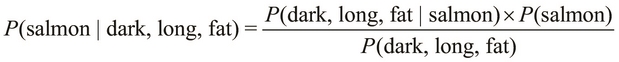

The terms, ![]() and
and ![]() , might seem a bit confusing, but the difference between these two terms is the order of occurrence of the specified conditions. The term,
, might seem a bit confusing, but the difference between these two terms is the order of occurrence of the specified conditions. The term, ![]() , represents the probability that a fish that is dark, long, and fat is a salmon, while the term,
, represents the probability that a fish that is dark, long, and fat is a salmon, while the term, ![]() , represents the probability that a salmon is a dark, long, and fat fish.
, represents the probability that a salmon is a dark, long, and fat fish.
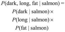
The ![]() probability can be calculated from the given training data as follows. As the three features of the fish are assumed to be mutually independent, the term,
probability can be calculated from the given training data as follows. As the three features of the fish are assumed to be mutually independent, the term, ![]() , is simply the product of the probabilities of the occurrences of each individual feature. By mutually independent, we mean that the variance or distribution of these features does not depend on any of the other features of the classification model.
, is simply the product of the probabilities of the occurrences of each individual feature. By mutually independent, we mean that the variance or distribution of these features does not depend on any of the other features of the classification model.
The term, ![]() , is also called the evidence of the given category, which is the category "salmon" in this case. We can express the
, is also called the evidence of the given category, which is the category "salmon" in this case. We can express the ![]() probability as the product of the probabilities of the independent features of the model; this is shown as follows:
probability as the product of the probabilities of the independent features of the model; this is shown as follows:
Interestingly, the terms, ![]() ,
, ![]() , and
, and ![]() , can be easily calculated from the training data and the
, can be easily calculated from the training data and the probability function, which we had implemented earlier. Similarly, we can find the probability that a fish is a salmon or ![]() . Thus, the only term that's not accounted for in the definition of
. Thus, the only term that's not accounted for in the definition of ![]() is the term,
is the term, ![]() . We can actually avoid calculating this term altogether using a simple trick in probability.
. We can actually avoid calculating this term altogether using a simple trick in probability.
Given that a fish is dark, long, and fat, it can either be a salmon or a sea bass. The two probabilities of occurrence of either category of fish are both complementary, that is, they both account for all the possible conditions that could occur in our model. In other words, these two probabilities both add up to a probability of 1. Thus, we can formally express the term, ![]() , as follows:
, as follows:
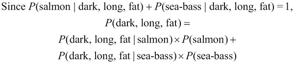
Both terms on the right-hand side of the preceding equality can be determined from the training data, which is similar to the terms, ![]() ,
, ![]() , and so on. Hence, we can calculate the
, and so on. Hence, we can calculate the ![]() probability directly from our training data. We express this probability through the following equality:
probability directly from our training data. We express this probability through the following equality:
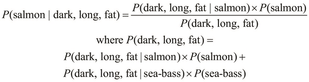
Now, let's implement the preceding equality using the training data and the probability function, which we defined earlier. Firstly, the evidence of a fish being a salmon, given that it's dark, long, and fat in appearance, can be expressed as follows:
(defn evidence-of-salmon [& attrs]
  (let [attr-probs (map #(probability % :category :salmon) attrs)
        class-and-attr-prob (conj attr-probs
                                  (probability :salmon))]
    (float (apply * class-and-attr-prob))))
To be explicit, we implement a function to calculate the probability of the term, ![]() , from the given training data. The equality of the terms,
, from the given training data. The equality of the terms, ![]() ,
, ![]() ,
, ![]() , and
, and ![]() will be used as a base for this implementation.
will be used as a base for this implementation.
In the preceding code, we determine the terms, ![]() and
and ![]() , for all the attributes or conditions of i by using the
, for all the attributes or conditions of i by using the probability function. Then, we multiply all these terms using a composition of the apply and * functions. Since all the calculated probabilities are ratios returned by the probability function, we cast the final ratio to a floating-point value using the float function . We can try out this function in the REPL as follows:
user> (evidence-of-salmon :dark)
0.4816
user> (evidence-of-salmon :dark :long)
0.2396884
user> (evidence-of-salmon)
0.6932
As the REPL output indicates, 48.16 percent of all the fish in the training data are salmon with dark skin. Similarly, 23.96 percent of all the fish are dark and long salmon, and 69.32 percent of all the fish are salmon. The value returned by the (evidence-of-salmon :dark :long) call can be expressed as ![]() , and similarly,
, and similarly, ![]() is returned by
is returned by (evidence-of-salmon).
Similarly, we can define the evidence-of-sea-bass function that determines the evidence of occurrence of a sea bass given some observed features of the fish. As we are dealing with only two categories, ![]() , we can easily verify this equality in the REPL. Interestingly, a small error is observed, but this error is not related to the training data. This small error is, in fact, a floating-point rounding error, which arises due to the limitations of floating-point numbers. In practice, we can avoid this using the decimal or
, we can easily verify this equality in the REPL. Interestingly, a small error is observed, but this error is not related to the training data. This small error is, in fact, a floating-point rounding error, which arises due to the limitations of floating-point numbers. In practice, we can avoid this using the decimal or BigDecimal (from java.lang) data types, instead of floating-point numbers. We can verify this using the evidence-of-sea-bass and evidence-of-salmon functions in the REPL as follows:
user> (+ (evidence-of-sea-bass) (evidence-of-salmon))
1.0000000298023224
We can generalize the evidence-of-salmon and evidence-of-sea-bass functions such that we are able to determine the probability of any category with some observed features; this is shown in the following code:
(defn evidence-of-category-with-attrs
  [category & attrs]
  (let [attr-probs (map #(probability % :category category) attrs)
        class-and-attr-prob (conj attr-probs
                                  (probability category))]
    (float (apply * class-and-attr-prob))))
The function defined in the preceding code returns values that agree with those returned by the following evidence-of-salmon and evidence-of-sea-bass functions:
user> (evidence-of-salmon :dark :fat)
0.38502988
user> (evidence-of-category-with-attrs :salmon :dark :fat)
0.38502988
Using the evidence-of-salmon and evidence-of-sea-bass functions, we can calculate the probability in terms of probability-dark-long-fat-is-salmon as follows:
(def probability-dark-long-fat-is-salmon
  (let [attrs [:dark :long :fat]
        sea-bass? (apply evidence-of-sea-bass attrs)
        salmon? (apply evidence-of-salmon attrs)]
    (/ salmon?
       (+ sea-bass? salmon?))))
We can inspect the probability-dark-long-fat-is-salmon value in the REPL as follows:
user> probability-dark-long-fat-is-salmon
0.957091799207812
The probability-dark-long-fat-is-salmon value indicates that a fish that is dark, long, and fat and has a 95.7 percent probability of being a salmon.
Using the preceding definition of the probability-dark-long-fat-is-salmon function as a template, we can generalize the calculations that it performs. Let's first define a simple data structure that can be passed around. In the spirit of idiomatic Clojure, we conveniently use a map for this purpose. Using a map, we can represent a category in our model along with the evidence and probability of its occurrence. Also, given the evidences for several categories, we can calculate the total probability of occurrence of a particular category as shown in the following code:
(defn make-category-probability-pair
  [category attrs]
  (let [evidence-of-category (apply
  evidence-of-category-with-attrs
                              category attrs)]
    {:category category
     :evidence evidence-of-category}))

(defn calculate-probability-of-category
  [sum-of-evidences pair]
  (let [probability-of-category (/ (:evidence pair)
                                   sum-of-evidences)]
    (assoc pair :probability probability-of-category)))
The make-category-probability-pair function uses the evidence-category-with-attrs function we defined in the preceding code to calculate the evidence of a category and its conditions or attributes. Then, it returns this value, as a map, along with the category itself. Also, we define the calculate-probability-of-category function, which calculates the total probability of a category and its conditions using the sum-of-evidences parameter and a value returned by the make-category-probability-pair function.
We can compose the preceding two functions to determine the total probability of all the categories given some observed values and then select the category with the highest probability, as follows:
(defn classify-by-attrs
  "Performs Bayesian classification of the attributes,
   given some categories.
   Returns a map containing the predicted category and
   the category's
   probability of occurrence."
  [categories & attrs]
  (let [pairs (map #(make-category-probability-pair % attrs)
                   categories)
        sum-of-evidences (reduce + (map :evidence pairs))
        probabilities (map #(calculate-probability-of-category
                              sum-of-evidences %)
                           pairs)
        sorted-probabilities (sort-by :probability probabilities)
        predicted-category (last sorted-probabilities)]
    predicted-category))
The classify-by-attrs function defined in the preceding code maps all the possible categories over the make-category-probability-pair function, given some conditions or observed values for the features of our model. As we are dealing with a sequence of pairs returned by make-category-probability-pair, we can use a simple composition of the reduce, map, and + functions to calculate the sum of all the evidence in this sequence. We then map the calculate-probability-of-category function over the sequence of category-evidence pairs and select the category-evidence pair with the highest probability. We do this by sorting the sequence through ascending probabilities and selecting the last element in the sorted sequence.
Now, we can use the classify-by-attrs function to determine the probability that an observed fish, which is dark, long, and fat, is a salmon. It is also represented by the probability-dark-long-fat-is-salmon value, which we defined earlier. Both expressions produce the same probability of 95.7 percent of a fish being a salmon, given that it's dark, long, and fat in appearance. We will implement the classify-by-attrs function as shown in the following code:
user> (classify-by-attrs [:salmon :sea-bass] :dark :long :fat)
{:probability 0.957091799207812, :category :salmon, :evidence 0.1949689}
user> probability-dark-long-fat-is-salmon
0.957091799207812
The classify-by-attrs function also returns the predicted category (that is, :salmon) of the given observed conditions :dark, :long, and :fat. We can use this function to tell us more about the training data as follows:
user> (classify-by-attrs [:salmon :sea-bass] :dark)
{:probability 0.8857825967670728, :category :salmon, :evidence 0.4816}
user> (classify-by-attrs [:salmon :sea-bass] :light)
{:probability 0.5362699908806723, :category :sea-bass, :evidence 0.2447}
user> (classify-by-attrs [:salmon :sea-bass] :thin)
{:probability 0.6369809383442954, :category :sea-bass, :evidence 0.2439}
As shown in the preceding code, a fish that is dark in appearance is mostly a salmon, and the one that is light in appearance is mostly a sea bass. Also, a fish that's thin is most likely a sea bass. The following values do, in fact, agree with the training data that we defined earlier:
user> (classify-by-attrs [:salmon] :dark)
{:probability 1.0, :category :salmon, :evidence 0.4816}
user> (classify-by-attrs [:salmon])
{:probability 1.0, :category :salmon, :evidence 0.6932}
Note that calling the classify-by-attrs function with only [:salmon] as a parameter returns the probability that any given fish is a salmon. An obvious corollary is that given a single category, the classify-by-attrs function always predicts the supplied category with complete certainty, that is, a probability of 1.0. However, the evidence returned by this function vary depending on the observed features passed to it as well as the sample data that we used to train our model.
In a nutshell, the preceding implementation describes a Bayes classifier that can be trained using some sample data. It also classifies some observed values for the features of our model.
We can describe a generic Bayes classifier by building upon the definition of the ![]() probability from our previous example. To quickly recap, the term
probability from our previous example. To quickly recap, the term ![]() can be formally expressed as follows:
can be formally expressed as follows:
In the preceding equality, we deal with a single class, namely salmon, and three mutually independent features, namely the length, width, and lightness of the skin of a fish. We can generalize this equality for N features as follows:
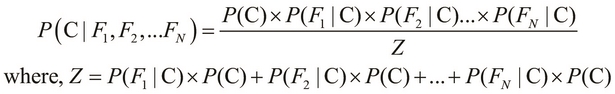
Here, the term Z is the evidence of the classification model, which we described in the preceding equation. We can use the sum and product notation to describe the preceding equality more concisely as follows:
The preceding equality describes the probability of occurrence of a single class, C. If we are given a number of classes to choose from, we must select the class with the highest probability of occurrence. This brings us to the basic definition of a Bayes classifier, which is formally expressed as follows:
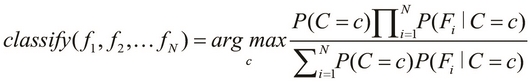
In the preceding equation, the function ![]() describes a Bayes classifier that selects the class with the highest probability of occurrence. Note that the terms
describes a Bayes classifier that selects the class with the highest probability of occurrence. Note that the terms ![]() represent the various features of our classification model, whereas the terms
represent the various features of our classification model, whereas the terms ![]() represent the set of observed values of these features. Also, the variable c, on the right-hand side of the equation, can have values from within a set of all the distinct classes in the classification model.
represent the set of observed values of these features. Also, the variable c, on the right-hand side of the equation, can have values from within a set of all the distinct classes in the classification model.
We can further simplify the preceding equation of a Bayes classifier via the Maximum a Posteriori (MAP) estimation, which can be thought of as a regularization of the features in Bayesian statistics. A simplified Bayes classifier can be formally expressed as follows:
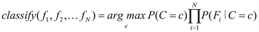
This definition essentially means that the classify function determines the class with the maximum probability of occurrence for the given features. Thus, the preceding equation describes a Bayes classifier that can be trained using some sample data and then be used to predict the class of a given set of observed values. We will now focus on using an existing implementation of a Bayes classifier to model a given classification problem.
The clj-ml library (https://github.com/joshuaeckroth/clj-ml) contains several implemented algorithms that we can choose from to model a given classification problem. This library is actually just a Clojure wrapper for the popular Weka library (http://www.cs.waikato.ac.nz/ml/weka/), which is a Java library that contains implementations for several machine learning algorithms. It also has several methods for evaluating and validating a generated classification model. However, we will concentrate on the clj-ml library's implementations of classifiers within the context of this chapter.
We'll now introduce the clj-ml library using an implementation of a Bayes classifier to model our previous problem involving the fish packaging plant. First, let's refine our training data to use numeric values rather than the keywords, which we described earlier, for the various features of our model. Of course, we will still maintain the partiality in our training data such that the salmon are mostly fat and dark-skinned, while the sea bass are mostly long and light-skinned. The following code implements this:
(defn rand-in-range
  "Generates a random integer within the given range"
  [min max]
  (let [len      (- max min)
        rand-len (rand-int len)]
    (+ min rand-len)))

;; sea bass are mostly long and light in color
(defn make-sea-bass []
  (vector :sea-bass
          (rand-in-range 6 10)          ; length
          (rand-in-range 0 5)           ; width
          (rand-in-range 4 10)))        ; lightness of skin

;; salmon are mostly fat and dark
(defn make-salmon []
  (vector :salmon
          (rand-in-range 0 7)           ; length
          (rand-in-range 4 10)          ; width
          (rand-in-range 0 6)))         ; lightness of skin
Here, we define the rand-in-range function, which simply generates random integers within a given range of values. We then redefine the make-sea-bass and make-salmon functions to use the rand-in-range function to generate values within the range of 0 and 10 for the three features of a fish, namely its length, width, and the darkness of its skin. A fish with a lighter skin color is indicated by a higher value for this feature. Note that we reuse the definitions of the make-sample-fish function and fish-dataset variable to generate our training data. Also, a fish is represented by a vector rather than a set, as described in the earlier definitions of the make-sea-bass and make-salmon functions.
We can create a classifier from the clj-ml library using the
make-classifier function, which can be found in the clj-ml.classifiers namespace. We can specify the type of classifier to be used by passing two keywords as arguments to the functions. As we intend to use a Bayes classifier, we supply the keywords, :bayes and :naive, to the make-classifier function. In a nutshell, we can use the following declaration to create a Bayes classifier. Note that the keyword, :naive, used in the following code signifies a naïve Bayes classifier that assumes that the features in our model are independent:
(def bayes-classifier (make-classifier :bayes :naive))
The clj-ml library's classifier implementations use datasets that are defined or generated using functions from the clj-ml.data namespace. We can convert the fish-dataset sequence, which is a sequence of vectors, into such a dataset using the make-dataset function. This function requires an arbitrary string name for the dataset, a template for each item in the collection, and a collection of items to add to the dataset. The template supplied to the make-dataset function is easily represented by a map, which is shown as follows:
(def fish-template
  [{:category [:salmon :sea-bass]}
   :length :width :lightness])

(def fish-dataset
  (make-dataset "fish" fish-template fish-training-data))
The fish-template map defined in the preceding code simply says that a fish, as represented by a vector, comprises the fish's category, length, width, and lightness of its skin, in that specific order. Note that the category of the fish is described using either :salmon or :sea-bass. We can now use fish-dataset to train the classifier represented by the bayes-classifier variable.
Although the fish-template map defines all the attributes of a fish, it's still lacking one important detail. It doesn't specify which of these attributes represent the class or category of the fish. In order to specify a particular attribute in the vector to represent the category of an entire set of observed values, we use the dataset-set-class function. This function takes a single argument that specifies the index of an attribute and is used to represent the category of the set of observed values in the vector. Note that this function does actually mutate or modify the dataset it's supplied with. We can then train our classifier using the classifier-train function, which takes a classifier and a dataset as parameters; this is shown in the following code:
(defn train-bayes-classifier []
  (dataset-set-class fish-dataset 0)
  (classifier-train bayes-classifier fish-dataset))
The preceding train-bayes-classifier function simply calls the dataset-set-class and classifier-train functions to train our classifier. When we call the train-bayes-classifier function, the classifier is trained with the following supplied data and then printed to the REPL output:
user> (train-bayes-classifier)
#<NaiveBayes Naive Bayes Classifier

                     Class
Attribute        salmon  sea-bass
                  (0.7)    (0.3)
=================================
length
  mean            2.9791   7.5007
  std. dev.       1.9897   1.1264
  weight sum        7032     2968
  precision            1        1

width
  mean            6.4822   1.9747
  std. dev.        1.706    1.405
  weight sum        7032     2968
  precision            1        1

lightness
  mean            2.5146   6.4643
  std. dev.       1.7047   1.7204
  weight sum        7032     2968
  precision            1        1

>
This output gives us some basic information about the training data, such as the mean and standard deviation of the various features that we model. We can now use this trained classifier to predict the category of a set of observed values for the features of our model.
Let's first define the observed values that we intend to classify. To do so, we use the following make-instance function, which requires a dataset and a vector of observed values that agree with the data template of the supplied dataset:
(def sample-fish
  (make-instance fish-dataset [:salmon 5.0 6.0 3.0]))
Here, we simply defined a sample fish using the make-instance function. We can now predict the class of the fish represented by sample-fish as follows:
user> (classifier-classify bayes-classifier sample-fish)
:salmon
As shown in the preceding code, the fish is classified as a salmon. Note that although we provide the class of the fish as :salmon while defining sample-fish, it's only for conformance with the data template defined by fish-dataset. In fact, we could specify the class of sample-fish as :sea-bass or a third value, say :unknown, to represent an undefined value, and the classifier would still classify sample-fish as a salmon.
When dealing with the continuous values for the various features of the given classification model, we can specify a Bayes classifier to use discretization of continuous features. By this, we mean that all the values for the various features of the model will be converted to discrete values by the probability density estimation. We can specify this option to the make-classifier function by simply passing an extra argument, {:supervised-discretization true}, to the function. This map actually describes all the possible options that can be provided to the specified classifier.
In conclusion, the clj-ml library provides a fully operational Bayes classifier that we can use to classify arbitrary data. Although we generated the training data ourselves in the previous example, this data can be fetched from the Web or a database as well.