The K-means clustering algorithm is a clustering technique that is based on vector quantization (for more information, refer to "Algorithm AS 136: A K-Means Clustering Algorithm"). This algorithm partitions a number of sample vectors into K clusters and hence derives its name. In this section, we will study the nature and implementation of the K-means algorithm.

Quantization, in signal processing, is the process of mapping a large set of values into a smaller set of values. For example, an analog signal can be quantized to 8 bits and the signal can be represented by 256 levels of quantization. Assuming that the bits represent values within the range of 0 to 5 volts, the 8-bit quantization allows a resolution of 5/256 volts per bit. In the context of clustering, quantization of input or output can be done for the following reasons:

The gist of the algorithm can be concisely described as follows. The K mean values, or centroids, are first randomly initialized. The distance of each sample value from each centroid is then calculated. A sample value is grouped into a given centroid's cluster depending on which centroid has the minimum distance from the given sample. In a multidimensional space for multiple features or input values, the distance of a sample input vector is measured by Euclidean distance between the input vector and a given centroid. This phase of the algorithm is termed as the assignment step.

The next phase in the K-means algorithm is the update step. The values of the centroids are adjusted based on the partitioned input values generated from the previous step. These two steps are then repeated until the difference between the centroid values in two consecutive iterations becomes negligible. Thus, the final result of the algorithm is the clusters or classes of each set of input values in the given training data.

The iterations performed by the K-means algorithm can be illustrated using the following plots:

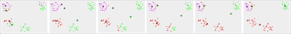
Each of the plots depict the centroid and partitioned sample values produced by each iteration of the algorithm for a given set of input values. The clusters in a given iteration are shown in different colors in each plot. The final plot represents the final partitioned set of input values produced by the K-means algorithm.

The optimization objective of the K-means clustering algorithm can be formally defined as follows:

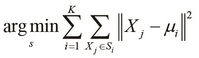
In the optimization problem defined in the preceding equation, the terms represent the K-mean values around which the input values are clustered. The K-means algorithm minimizes the size of the clusters and also determines the mean values for which these clusters can be minimized in size.

This algorithm requires sample values and initial mean values as inputs. In the assignment step, the input values are assigned to clusters around the initial mean values supplied to the algorithm. In the later update step, the new mean values are calculated from the input values. In most implementations, the new mean values are calculated as the mean of all input values that belongs to a given cluster.

Most implementations initialize the initial mean values to some randomly chosen input values. This technique is called the Forgy method of random initialization.

The K-means algorithm is NP-hard when either the number of clusters K or the number of dimensions in the input data d is unbound. When both these values are fixed, the K-means algorithm has a time complexity of . There are several variations of this algorithm that vary on how the new mean values are calculated.

We will now demonstrate how we can implement the K-means algorithm in pure Clojure, while using no external libraries. We begin by defining bits and pieces of the algorithm, which are then later combined to provide a basic visualization of the K-means algorithm.

We can say that the distance between two numbers is the absolute difference between their values and this can be implemented as a distance function, as shown in the following code:

(defn distance [a b]
  (if (< a b) (- b a) (- a b)))

If we are given a number of mean values, we can calculate the closest mean from a given number by using a composition of the distance and sort-by functions, as shown in the following code:

(defn closest [point means distance]
  (first (sort-by #(distance % point) means)))

To demonstrate the closest function defined in the preceding code, we will first need to define some data, that is, a sequence of numbers and a couple of mean values, as shown in the following code:

(def data '(2 3 5 6 10 11 100 101 102))
(def guessed-means '(0 10))

We can now use the data and guessed-means variables with the closest function and an arbitrary number, as shown in the following REPL output:

user> (closest 2 guessed-means distance)
0
user> (closest 9 guessed-means distance)
10
user> (closest 100 guessed-means distance)
10

Given the means 0 and 10, the closest function returns 0 as the closest mean to 2, and 10 as that for 9 and 100. Thus, a set of data points can be grouped by the means, which are closest to them. We can implement a function that implements this grouping operation using the closest and group-by functions as follows:

(defn point-groups [means data distance]
  (group-by #(closest % means distance) data))

The point-groups function defined in the preceding code requires three arguments, namely the initial mean values, the collection of points to be grouped, and lastly a function that returns the distance of a point from a given mean. Note that the group-by function applies a function, which is passed as the first parameter, to a collection, which is then passed as the second parameter.

We can apply the point-groups function on the list of numbers represented by the data variable to group the given values by their distance from the guessed means, represented by guessed-means as shown in the following code:

user> (point-groups guessed-means data distance)
{0 [2 3 5], 10 [6 10 11 100 101 102]}

As shown in the preceding code, the point-groups function partitions the sequence data into two groups. To calculate the new set of mean values from these groups of input values, we must calculate their average value, which can be implemented using the reduce and count functions, as shown in the following code:

(defn average [& list]
  (/ (reduce + list)
     (count list)))

We implement a function to apply the average function defined in the preceding code to the previous mean values and the map of groups returned by the point-groups function. We will do this with the help of the following code:

(defn new-means [average point-groups old-means]
  (for [m old-means]
    (if (contains? point-groups m)
      (apply average (get point-groups m)) 
      m)))

In the new-means function defined in the preceding code, for each value in the previous mean values, we apply the average function to the points that are grouped by the mean value. Of course, the average function must be applied to the points of a given mean only if the mean has any points grouped by it. This is checked using the contains? function in the new-means function. We can inspect the value returned by the new-means function on our sample data in the REPL, as shown in the following output:

user> (new-means average
        (point-groups guessed-means data distance)
                 guessed-means)
(10/3 55)

As shown in the preceding output, the new mean values are calculated as (10/3 55) from the initial mean values (0 10). To implement the K-means algorithm, we must apply the new-means function iteratively over the new mean values returned by it. This iteration can be performed using the iterate function, which requires a function that takes a single argument to be passed to it.

We can define a function to use with the iterate function by currying the new-means function over the old mean values passed to it, as shown in the following code:

(defn iterate-means [data distance average]
  (fn [means]
    (new-means average
               (point-groups means data distance)
               means)))

The iterate-means function defined in the preceding code returns a function that calculates the new mean values from a given set of initial mean values, as shown in the following output:

user> ((iterate-means data distance average) '(0 10))
(10/3 55)
user> ((iterate-means data distance average) '(10/3 55))
(37/6 101)

As shown in the preceding output, the mean value is observed to change on applying the function returned by the iterate-means function a couple of times. This returned function can be passed to the iterate function and we can inspect the iterated mean values using the take function, as shown in the following code:

user> (take 4 (iterate (iterate-means data distance average)
                       '(0 10)))
((0 10) (10/3 55) (37/6 101) (37/6 101))

It's observed that the mean value changes only in the first three iterations and converges to the value (37/6 10) for the sample data that we have defined. The termination condition of the K-means algorithm is the convergence of the mean values and thus we must iterate over the values returned by the iterate-means function until the returned mean value does not differ from the previously returned mean value. Since the iterate function lazily returns an infinite sequence, we must implement a function that limits this sequence by the convergence of the elements in the sequence. This behavior can be implemented by lazy realization using the lazy-seq and seq functions as shown in the following code:

(defn take-while-unstable
  ([sq] (lazy-seq (if-let [sq (seq sq)]
                    (cons (first sq)
                          (take-while-unstable 
                           (rest sq) (first sq))))))
  ([sq last] (lazy-seq (if-let [sq (seq sq)]
                         (if (= (first sq) last)
                           nil
                           (take-while-unstable sq))))))

The take-while-unstable function defined in the preceding code splits a lazy sequence into its head and tail terms and then compares the first element of the sequence with the first element of the tail of the sequence to return an empty list, or nil, if the two elements are equal. However, if they are not equal, the take-while-unstable function is invoked again on the tail of the sequence. Note the use of the if-let macro, which is simply a let form with an if expression as its body to check if the sequence sq is empty. We can inspect the value returned by the take-while-unstable function in the REPL as shown in the following output:

user> (take-while-unstable
       '(1 2 3 4 5 6 7 7 7 7))
(1 2 3 4 5 6 7)
user> (take-while-unstable 
       (iterate (iterate-means data distance average)
                '(0 10)))
((0 10) (10/3 55) (37/6 101))

Using the final mean value we have calculated, we can determine the clusters of input values using the vals function on the map returned by the point-groups function, as shown in the following code:

(defn k-cluster [data distance means]
  (vals (point-groups means data distance)))

Note that the vals function returns all the values in a given map as a sequence.

The k-cluster function defined in the preceding code produces the final clusters of input values returned by the K-means algorithm. We can apply the k-cluster function on the final mean value (37/6 101) to return the final clusters of input values, as shown in the following output:

user> (k-cluster data distance '(37/6 101))
([2 3 5 6 10 11] [100 101 102])

To visualize the change in the clusters of input values, we can apply the k-cluster function on the sequence of values returned by composing the iterate and iterate-means functions. We must limit this sequence by convergence of the values in all clusters and this can be done using the take-while-unstable function, as shown in the following code:

user> (take-while-unstable
       (map #(k-cluster data distance %)
            (iterate (iterate-means data distance average)
             '(0 10))))
(([2 3 5] [6 10 11 100 101 102])
 ([2 3 5 6 10 11] [100 101 102]))

We can refactor the preceding expression into a function that requires only the initial set of guessed mean values by binding the iterate-means function to the sample data. The functions used to calculate the distance of a given input value from a mean value and the average mean value from a set of input values are as shown in the following code:

(defn k-groups [data distance average]
  (fn [guesses]
    (take-while-unstable
     (map #(k-cluster data distance %)
          (iterate (iterate-means data distance average)
                   guesses)))))

We can bind the k-groups function defined in the preceding code with our sample data and the distance and average functions, which operate on numeric values as shown in the following code:

(def grouper
  (k-groups data distance average))

Now, we can apply the grouper function on any arbitrary set of mean values to visualize the changes in the clusters over the various iterations of the K-means algorithm, as shown in the following code:

user> (grouper '(0 10))
(([2 3 5] [6 10 11 100 101 102])
 ([2 3 5 6 10 11] [100 101 102]))
user> (grouper '(1 2 3))
(([2] [3 5 6 10 11 100 101 102])
 ([2 3 5 6 10 11] [100 101 102])
 ([2 3] [5 6 10 11] [100 101 102])
 ([2 3 5] [6 10 11] [100 101 102])
 ([2 3 5 6] [10 11] [100 101 102]))
user> (grouper '(0 1 2 3 4))
(([2] [3] [5 6 10 11 100 101 102])
 ([2] [3 5 6 10 11] [100 101 102])
 ([2 3] [5 6 10 11] [100 101 102])
 ([2 3 5] [6 10 11] [100 101 102])
 ([2] [3 5 6] [10 11] [100 101 102])
 ([2 3] [5 6] [10 11] [100 101 102]))

As we mentioned earlier, if the number of mean values is greater than the number of inputs, we end up with a number of clusters equal to the number of input values, in which each cluster contains a single input value. This can be verified in the REPL using the grouper function, as shown in the following code:

user> (grouper (range 200))
(([2] [3] [100] [5] [101] [6] [102] [10] [11]))

We can extend the preceding implementation to apply to vector values and not just numeric values, by changing the distance and average distance, which are parameters to the k-groups function. We can implement these two functions for vector values as follows:

(defn vec-distance [a b]
  (reduce + (map #(* % %) (map - a b))))

(defn vec-average [& list]
  (map #(/ % (count list)) (apply map + list)))

The vec-distance function defined in the preceding code implements the squared Euclidean distance between two vector values as the sum of the squared differences between the corresponding elements in the two vectors. We can also calculate the average of some vector values by adding them together and dividing each resulting element by the number of vectors that were added together, as shown in the vec-average function defined in the preceding code. We can inspect the returned values of these functions in the REPL as shown in the following output:

user> (vec-distance [1 2 3] [5 6 7])
48
user> (vec-average  [1 2 3] [5 6 7])
(3 4 5)

We can now define some of the following vector values to use as sample data for our clustering algorithm:

(def vector-data
  '([1 2 3] [3 2 1] [100 200 300] [300 200 100] [50 50 50]))

We can now use the k-groups function with the vector-data, vec-distance, and vec-average variables to print the various clusters iterated through to produce the final set of clusters, as shown in the following code:

user> ((k-groups vector-data vec-distance vec-average)
       '([1 1 1] [2 2 2] [3 3 3]))
(([[1 2 3] [3 2 1]] [[100 200 300] [300 200 100] [50 50 50]])

 ([[1 2 3] [3 2 1] [50 50 50]]
  [[100 200 300] [300 200 100]])

 ([[1 2 3] [3 2 1]]
  [[100 200 300] [300 200 100]]
  [[50 50 50]]))

Another improvement we can add to this implementation is updating identical mean values by the new-means function. If we pass a list of identical mean values to the new-means function, both the mean values will get updated. However, in the classic K-means algorithm, only one mean from two identical mean values is updated. This behavior can be verified in the REPL, by passing a list of identical means such as '(0 0) to the new-means function, as shown in the following code:

user> (new-means average 
                 (point-groups '(0 0) '(0 1 2 3 4) distance) 
                 '(0 0))
(2 2)

We can avoid this problem by checking the number of occurrences of a given mean in the set of mean values and only updating a single mean value if multiple occurrences of it are found. We can implement this using the frequencies function, which returns a map with keys as elements from the original collection passed to the frequencies function and values as the frequencies of occurrences of these elements. We can thus redefine the new-means function, as shown in the following code:

(defn update-seq [sq f]
  (let [freqs (frequencies sq)]
    (apply concat
     (for [[k v] freqs]
       (if (= v 1) 
         (list (f k))
         (cons (f k) (repeat (dec v) k)))))))
(defn new-means [average point-groups old-means]
  (update-seq
   old-means
   (fn [o]
     (if (contains? point-groups o)
       (apply average (get point-groups o)) o))))

The update-seq function defined in the preceding code applies a function f to the elements in a sequence sq. The function f is only applied to a single element if the element is repeated in the sequence. We can now observe that only a single mean value changes when we apply the redefined new-means function on the sequence of identical means '(0 0), as shown in the following output:

user> (new-means average
                 (point-groups '(0 0) '(0 1 2 3 4) distance)
                 '(0 0))
(2 0)

A consequence of the preceding redefinition of the new-means function is that the k-groups function now produces identical clusters when applied to both distinct and identical initial mean values, such as '(0 1) and '(0 0), as shown in the following code:

user> ((k-groups '(0 1 2 3 4) distance average)
       '(0 1))
(([0] [1 2 3 4]) ([0 1] [2 3 4]))
user> ((k-groups '(0 1 2 3 4) distance average)
       '(0 0))
(([0 1 2 3 4]) ([0] [1 2 3 4]) ([0 1] [2 3 4]))

This new behavior of the new-means function with respect to identical initial mean values also extends to vector values as shown in the following output:

user> ((k-groups vector-data vec-distance vec-average)
       '([1 1 1] [1 1 1] [1 1 1]))
(([[1 2 3] [3 2 1] [100 200 300] [300 200 100] [50 50 50]])
 ([[1 2 3] [3 2 1]] [[100 200 300] [300 200 100] [50 50 50]])
 ([[1 2 3] [3 2 1] [50 50 50]] [[100 200 300] [300 200 100]])
 ([[1 2 3] [3 2 1]] [[100 200 300] [300 200 100]] [[50 50 50]]))

In conclusion, the k-cluster and k-groups functions defined in the preceding example depict how K-means clustering can be implemented in idiomatic Clojure.

[cc.artifice/clj-ml "0.4.0"]
[incanter "1.5.4"]

(ns my-namespace
  (:use [incanter core datasets]
        [clj-ml data clusterers]))

(def features [:Sepal.Length
               :Sepal.Width
               :Petal.Length
               :Petal.Width])

(def iris-data (to-vect (sel (get-dataset :iris)
                             :cols features)))

(def iris-dataset
  (make-dataset "iris" features iris-data))

user> iris-dataset
#<ClojureInstances @relation iris

@attribute Sepal.Length numeric
@attribute Sepal.Width numeric
@attribute Petal.Length numeric
@attribute Petal.Width numeric

@data
5.1,3.5,1.4,0.2
4.9,3,1.4,0.2
4.7,3.2,1.3,0.2
...
4.7,3.2,1.3,0.2
6.2,3.4,5.4,2.3
5.9,3,5.1,1.8>

(def k-means-clusterer
  (make-clusterer :k-means
                  {:number-clusters 3}))

(defn train-clusterer [clusterer dataset]
  (clusterer-build clusterer dataset)
  clusterer)

user> (train-clusterer k-means-clusterer iris-dataset)
#<SimpleKMeans
kMeans
======

Number of iterations: 6
Within cluster sum of squared errors: 6.982216473785234
Missing values globally replaced with mean/mode

Cluster centroids:
                            Cluster#
Attribute       Full Data          0          1          2
                    (150)       (61)       (50)       (39)
==========================================================
Sepal.Length       5.8433     5.8885      5.006     6.8462
Sepal.Width        3.0573     2.7377      3.428     3.0821
Petal.Length        3.758     4.3967      1.462     5.7026
Petal.Width        1.1993      1.418      0.246     2.0795

user> (clusterer-cluster k-means-clusterer iris-dataset)
#<ClojureInstances @relation 'clustered iris'

@attribute Sepal.Length numeric
@attribute Sepal.Width numeric
@attribute Petal.Length numeric
@attribute Petal.Width numeric
@attribute class {0,1,2}

@data
5.1,3.5,1.4,0.2,1
4.9,3,1.4,0.2,1
4.7,3.2,1.3,0.2,1
...
6.5,3,5.2,2,2
6.2,3.4,5.4,2.3,2
5.9,3,5.1,1.8,0>