
CHAPTER 4
PROMOTER RECOGNITION USING NEURAL NETWORK APPROACHES
4.1 INTRODUCTION
Currently, huge amount of genome data is available due to fast sequencing methods. Similar fast annotation methods of the genome are not available and current technologies consume a lot of time. Hence, machine annotation methods are required to tackle the major problems of promoter recognition and gene recognition.
Promoters occur upstream of a gene and are regions at which ribonucleic acid (RNA) polymerase binds and initiates transcription. Promoters also act as switches specifying the location in the organism, as well as the time at which the transcription can occur at that gene. The location where transcription begins is known as the transcription start site (TSS). A majority of the promoters of genes that transcribe large amounts of messenger RNA (mRNA) have a set of binding sites or regions [1,2]. One of these sites is a TATA sequence, a hexamer, upstream from TSS. Promoter also contains one or more binding regions further upstream and downstream. The eukaryotic and prokaryotic promoter recognition problems have to be dealt with independently. For example, the promoter structure for Escherichia coli has two binding regions present at -10 and -35 positions with respect to TSS (position of which is taken as +1). These are indicated as a -35 motif and a -10 motif. The patterns at these binding sites are known to be conserved. In general, patterns (TATA box, CAAT box, Initiator, etc.) are known to be conserved in the promoter sequences within and across species in some cases.
The distinct feature in case of eukaryotic transcription is that the RNA polymerase does not bind to the promoter directly. A number of transcription-binding proteins bind to the binding sites and form a complex before RNA polymerase binds. Also, there are three kinds of RNA polymerase in eukaryotes unlike the prokaryotes. For the proteins to bind to deoxyribonucleic acid (DNA), it has to have a physical structure wherein the proteins can come and bind. Special proteins that are used for this purpose are Helix turn Helix, and Zn++ fingers.
Promoter recognition is not a trivial problem due to the following reasons: Promoter recognition unlike other recognition problems (e.g., exon prediction and gene recognition) does not yield good results with methods of alignment or sequence similarity searches, since promoters have very low sequence similarity. Though the patterns (e.g., TATA box) are known to be conserved, there exist many exceptions to this rule. Nonconservation and distance between the patterns, the presence or absence of the patterns themselves make the task of promoter prediction an even more complex problem. Also, the occurrence of a promoter is not restricted to the 5’ end of a gene alone, but could in fact be found in a coding region or may overlap with another promoter in the case of prokaryotes. Additionally, in the case of eukaryotes, promoters additionally may exist in an intron or in the untranslated region of 3’. Hence, the problem of recognition of promoter against various backgrounds gains importance computationally.
Recently, there has been a deluge of sequencing information due to efficient sequencing methods. Several mammalian, bacterial, and plant species have been sequenced. One can use experimental methods [e.g., DNA footprinting, DNA protein cross-linking, X-ray crystallography, and nuclear magnetic resonance (NMR) spectroscopy] to identify a promoter or a gene. Typically, there are millions of protein sequences, but experimentally determined protein structures are only on the order of 1000. Experimental methods to determine a promoter, a gene, or a protein structure are time-consuming processes. Hence, annotation of important regions (e.g., genes) is not very fast. To overcome this handicap, computational techniques or algorithms that can automatically identify these regions are required.
4.2 RELATED LITERATURE /BACKGROUND
The crux of the problem is to identify a promoter irrespective of its place of occurrence in the genome, by extracting features that are unique to it. Different research groups have been trying to identify these patterns or features specific for promoters by various feature extraction methods and different classifiers.
Machine learning techniques can be used to address the issues mentioned above by modeling the recognition–prediction problem as a pattern recognition problem. To properly classify the promoter sequences in silico, one should get features that capture the essence of promoters. Some of the popular feature extraction methods are based on genetic algorithms [4], statistical models (e.g., hidden Markov models [5] and position weight matrices [6–8]), syntactic recognition algorithms [9], expectation, and maximization method [10,11].
Methods based on features extracted from the binding sites or local consensus regions can be termed as local signal-based methods. Position weight matrices, expectation and maximization algorithm, and hidden Markov models have been used in the literature to extract local signals for the promoter recognition problem cite{Bajic2002a, Cardon, Pedersen}. Local signal-based methods for eukaryotic promoter recognition use specific motifs like the four binding sites: The TATA box, the initiator (Inr) region, an upstream activating element (UPE), and a downstream promoter element (DPE). The detection of transcription factor binding sites forms the core of the local signal-based methods.
The techniques that use the whole promoter sequence to extract features can be categorized as global signal-based methods. Techniques like Fourier transform (FT), sequence alignment method, and so on, fall under this category. Global signal-based methods use properties, such as GpC content, secondary structure elements, and cruciform DNA structure, for eukaryotic promoter recognition [12]. The literature is abundant with local signal-based methods. Global signal-based methods are also catching up. Some of the work on the promoter recognition problem of both these kinds, which were carried out in the last few years, is presented in Section 4.3.
Das and Dai [13] present a comprehensive literature survey on the DNA motif finding algorithms. Motifs generally searched in the promoter sequences of coregulated genes and more recently integrated approaches that include phylogenetic footprinting are being used to find motifs. This survey gives a view of the local signal-based methods that are used to extract conserved patterns in the DNA promoter sequences. Huerta and Collado-Vides created an E. coli promoter data set called Regulon database [14]. They extracted and aligned motifs in a given set of unordered sequences producing a frequency matrix. A set of 96 different weight matrices were created for promoter, coding, and noncoding regions. A score is computed using these weight matrices and the best weight matrix is used to predict a promoter. The predictive capacity of the method is 86%, however, accuracy defined as the average of sensitivity and positive predictive rate, is 53%. An important contribution of this work is that they predict a high number of putative promoters (promoter-like signals) in the vicinity of a true promoter, which show a better score than the true promoter. The authors suggest that these putative promoters may be trying to bring Ribonucleic polymerase (RNAP) closer to the functional promoter.
Bajic et al. designed a local signal-based algorithm that combines a nonlinear promoter recognition model with signal processing, artificial neural networks (ANNs), and a set of sensors in Dragon fly (Drosophila melanogaster) promoter prediction [6]. These sensors are based on the statistical concept of oligonucleotide positional distributions in specific functional regions of DNA. Each sensor models a particular functional region (e.g., promoter, coding-exon, and intron). These distributions are modeled as a set of position weight matrices of the most significant oligonucleotides. Pentamers (regions of length 5) that most significantly contribute to the separation between the promoter and nonpromoter regions are chosen by determining the significance using their statistical relevance. The signals of a sequence using the positional weight matrices for the three functional regions are fed to a signal processing block. The output is fed to ANN, which performs multisensor integration. Scores that make the ANN output greater than the selected threshold are to be treated as positive predictions in the promoter region. They have obtained a sensitivity rate of 67%. The authors have shown that their methods predict less false positives compared to the then existing algorithms.
Levitsky and Katokhin [4] have used the genetic algorithm based on iterative discriminant analysis, which is based on a global signal to classify eukaryotic (Drosophila) promoters. The negative set is obtained by shuffling the promoters. Two promoter sample TATA and DPE containing sets are formed. The cross-correlation (CC) for TATA containing promoters is reported to be 0.92 and for DPE is shown to be 0.82.
Pedersen et al. characterized the promoters of prokaryotes (E. coli) and eukaryotes (human) using self-organizing parallel HMMs [5]. They considered a set of three states (the main, the delete, and the insertion states), in addition to start and end states. The set of emissions are the four nucleotides A,T,G,C. Main and insertion states always emit a nucleotide, whereas the deletion state is a no-emission state (i.e., a mute state). Given a set of K training sequences, the parameters of HMM are iteratively modified to optimize the data fit using a measure based on the log-likelihood. A set of HMMs trained on 38 σ70, and 3 σ54 sequences are combined in parallel to create a super HMM for E. coli promoter recognition. Similarly, human promoter sequences are used to train another HMM model. Clear patterns of well-known consensus signals (TATA box, etc.) could be obtained from the emission probabilities of main states of the HMM model. Their model is able to classify 162 σ70 out of 166 sequences as σ70 and 3 σ54 out of 166 as σ54 sequences. Only one σ70 sequence out of 166 is misclassified. They have not been tested on nonpromoter sequences.
It is said that DNA encodes two levels of functional information. The first level is for proteins and targets for activators, enhancers, repressors, transcription factor binders, and so on. The second level of information is contained in the physical and structural properties of the DNA itself [15,16]. In the literature, several groups have exploited these properties to distinguish between features specific to a particular set of a DNA sequences and sequences that do not belong to a particular set. Physico-chemical parameters of a DNA double strand are available in the literature [16]. Kobe et al., reviewed the work of other groups that have considered the structural properties specific to mammals and plants [17]. There are some groups who have encoded the DNA independent of these properties in terms of binary values. Whatever encoding is used, the whole sequence is considered for modeling in global signal-based methods. Conformational and physicochemical properties of B-DNA dinucleotides [16] tabulated by the author and are used as global features for promoter recognition.
This chapter presents our work, which is based on global signal-based methods using a neural network classifier. For this purpose, we considered two global features: n-gram features and features based on signal processing techniques. It is shown that the n-gram features extracted for n=2,3,4,5 efficiently discriminate promoters from nonpromoters.
4.3 GLOBAL SIGNAL-BASED METHODS FOR PROMOTER RECOGNITION
Promoter recognition has been conventionally attempted using binding-site prediction algorithms that are primarily based on motif search techniques. We believe that along with binding sites, the upstream and downstream regions contribute to the function of the promoter, and hence we do an indepth study of the entire promoter region. There is an indication that codons that are triplets constitute useful features [18] in a DNA sequence and also the promoter regions are shown to have conserved hexamers [19]. On the other hand, to compute hexamers that will be 46 in number for every DNA sequence is computationally expensive. We present our study of the promoter region using n-gram features that are contiguous blocks of n characters from a sequence for n=2,3,4, and 5.
Traditionally, biomedical signals have been analyzed by signal processing techniques [e.g., FT and wavelet transforms]. Biological data sets consist mostly of sequences made up of either nucleotides or amino acids. Hence, an encoding system is required to convert these sequences into numerical series. Once a numerical series is obtained, FT or wavelet transform (WT) can be applied. Wavelets have been used in the literature to analyze biological signals (e.g., genome sequences, protein structures, and gene expression data) [20]. It is assumed that the promoter signal that is responsible for the binding is retained by the promoter whether it occurs in an inter-genic portion or in a coding region [21]. To start with, FT of the sequences is used to analyze the promoter region to gain knowledge in the frequency domain. Fourier transform per se cannot be used for promoter recognition. Hence, its power spectrum computed using the Fourier coefficients are used as features. Since in FT, positional information is lost, WT is being used to retain that information. Promoter recognition is posed as a binary classification problem. So far FT has been used by quite a few groups, but there is no work, as far as we know, which uses wavelets for promoter recognition.
4.3.1 Data Set
This section describes the prokaryotic and eukaryotic data sets that are used for promoter recognition problem and the n-gram feature extraction methods used for experimentation.
The prokaryotic data set of E. coli is built by taking 669 σ-70 promoter sequences of length 80 with 60 base pairs (bp) upstream of the TSS and the rest downstream as is proposed in the literature from RegulonDB and Promec data bases [22]. Both the positive and the negative data sets are obtained from Gordon et al. [22]. There is no standard negative data set available. Gordon et al., build the negative data set by choosing sequence fragments outside the promoter region. This is a biologically meaningful data set that consists of 709 sequence fragments from the coding region and 709 sequence segments from intergenic portions.
The eukaryotic promoter data set of Drosophila is obtained from Ohler et al. [23], which is taken from the eukaryotic promoter database (EPD) [24]. A negative data set is built by them from the Drosophila genome [23]. Sequences from both positive and negative data sets are of length 300 bp with 250 bp upstream of the TSS and the rest is downstream. The data set contains 1864 promoter sequences, 2859 from coding and 1799 sequences from intron portions.
4.3.2 Promoter Recognition Using n-Gram Features
A few research papers on protein sequence classification and gene identification that use n-grams are seen, but very few are available in the literature that are applied to promoter recognition. A new class of variable-order Bayesian network models (VOBN) is proposed by Ben-gal et al. [25]. These models generalize the widely used position weight matrix (PWM), Markov, and Bayesian network models. Instead of considering a fixed subset of the positions to model dependencies, in VOBN models, these subsets may vary based on the specific nucleotides observed, which are called the context. The VOBN model is applied to a set of 238 σ70 binding sites in E. coli. The authors show that the VOBN model can distinguish those 238 sites from a set of 472 intergenic nonpromoter sequences with higher accuracy than fixed-order Markov models or Bayesian trees. They consider the statistical dependencies between adjacent base pairs of nucleotides in E. coli to achieve a true positive recognition rate of 47.56% [25].
Leu et al. used n-gram features for n = 6–20 to predict promoters for vertebrates [26]. They consider sequences of length 550 bp. Each sequence segment of length 200 bp is given a cumulative score using all these n-grams with the individual n-gram score designed based on its occurrence only in promoter or in nonpromoter or in both promoter and nonpromoter. They achieve an accuracy rate of 88% with this method. Ji et al. implemented support vector machine using n-gram features (n = 4,5,6,7) for target gene prediction of Arabidopsis [27].
Wang and Hannenhalli proposed a position specific propensity analysis model (PSPA), which extracts the propensity of DNA elements at a particular position and their cooccurrence with respect to TSS in mammals [28]. They considered a set of top ranking k-mers (k = 1–5) at each position ±100 bp relative to TSS and computed the cooccurrence with other top-ranking k-mers at other downstream positions. The PSPA score for a sequence is computed as the product of scores for the 200 positions of ±100 bp relative to TSS. They found many position-specific promoter elements that are strongly linked to gene product function.
Li and Lin considered position-specific weight matrices of hexamers at 10 specific positions for the promoter data of E. coli [29]. The position correlation scoring matrix (PCSM) is computed for promoter as well as the nonpromoter set of training sequences. If the score is higher for positive than in the negative PCSM, then the test sequence is identified as a promoter and similarly nonpromoters are identified. Li and Lin [28] report performance of sensitivity being 91% and specificity 81% for nonpromoter data consisting of coding regions alone and 90 and 77% for nonpromoter data taken from inter-genic portions only. Applying these scores to the whole genome to predict the promoters, all 683 experimentally verified σ-70 promoters are successfully predicted and 1567 predictions as probable promoters.
More recently, Sonnenburg et al. introduced the positional oligomer importance matrices (POIMs) that are k-mer based scoring schemes and proposed an efficient algorithm to compute the scores for k-mers [30]. The POIMs can be utilized to recognize transcription start, trans-splicing sites (TRSSs) and acceptor splice sites. They showed that POIMs can recover many known motifs whose length, location, and typical sequences of motifs can be obtained accurately by these matrices.
Rani and Bapi carried out a study of different n-grams (n = 2,3,4, and 5) and their suitability as features for the promoter recognition problem posed as a binary classification problem [31]. The authors have chosen genomes of E. coli from prokaryotes and the method is extended to the eukaryote D. melanogaster promoter prediction. In [32], an investigation was made using dinucleotide frequencies as features in promoter recognition. The emphasis here was on analyzing misclassified sequences in both promoter and nonpromoter data sets. Further, in [31], a global view of the whole promoter is attempted using a systematic study of n-grams as features for promoter recognition. The whole promoter sequence is considered for the prediction and no position specific information is used. In Section 4.3.2.1, details of this work are presented.
4.3.2.1 n-Gram Extraction A global signal is extracted from the promoter sequence by looking at the frequency of occurrence of n-grams in the promoter region. The set of n-grams for n = 2 is 16 possible combinations of features (AA, AT, AG, AC, TA, etc.) and the set of n-grams for n = 3 are 64 triples (AAA, AAT, AAG, AAC, ATA, etc.). The frequency of occurrence of n-grams is calculated on the DNA alphabet {A,T,G,C} for n = 2, 3, 4, and 5. Let fi(n) denote the frequency of occurrence of the ith feature of n-grams for a particular n value and let L denote the length of the sequence. The feature values vi(n) are normalized frequency counts given in the following equation:
Here, the denominator denotes the number of n-grams that are possible in a sequence of length L. Hence, vi(n) denotes the proportional frequency of occurrence of ith feature for a particular n value. Thus each promoter and nonpromoter sequence of the data set is represented as a 16-dimensional feature vector (v1(2), 2(2),…,v16(2)) for n = 2, as a 64-dimensional feature vector (v1(3), 2(3), …, v64(3)) for n = 3, and so on, and a 1024-dimensional feature vector (v1(5), 2(5),…,v1024(5)) for n = 5.
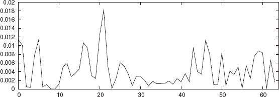
The feature vectors for promoter and nonpromoter sequences constitute the entire data set. A portion of the data set is used as the training set and the remaining as a test set in this binary classification problem. The data sets are well separated in the feature spaces fi(n) for n = 2, 3, 4, and 5. As an illustration, the average separation between promoter and nonpromoter sequences for 3-grams is shown in Figure 4.1. A neural network classifier is trained using n-grams of the training set as input feature vectors and then the test set is evaluated using the same network.
FIGURE 4.1 Average separation between promoter and nonpromoter sequences for 3-grams for E. coli. On the x-axis, 0,…,63 denotes 3-grams AAA, AAT, AAG, AAC, …, CCG, CCC.
4.3.2.2 Neural Network Classification Performance Promoter classification is obtained using a multilayer perceptron having three layers, namely, an input, a hidden, and an output layer. The output layer has one node to give a binary decision as to whether the given input sequence is a promoter or nonpromoter. The input layer contains 16, 64, 256, and 1024 nodes corresponding to the n-gram features for n = 2,3,4, and 5, respectively. Different experiments are carried out to find the optimal number of hidden nodes that give the best classification performance. In a fivefold cross-validation, 80% of the data set is used for training the network and the remaining 20% is used as the test data set. Average performance of the neural network over fivefolds is reported in order to evaluate the efficacy of the various n-gram features for promoter classification. These simulations are done using the Stuttgart neural network simulator [33].
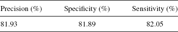
The classification results are evaluated on the test data set using different performance measures (e.g., precision, specificity and sensitivity, and positive predictive value). Precision is the proportion of the correctly classified sequences of the entire test data set. Specificity is the proportion of the negative test sequences that are correctly classified and sensitivity is the proportion of the positive test sequences that are correctly classified. Positive predictive value (PPV) is defined as the proportion of true positives with respect to the total number of sequences that are predicted as positive (true positives + false positives).
Using this architecture of the neural network, promoter classification is carried out for E. coli and Drosophila for n = 2,3,4, and 5 grams. It is found in E. coli that PPV for 2, 3, 4, and 5-grams is 81.29, 82.97, 80.03, and 81.09, respectively, and the percentage of PPV obtained for Drosophila is 85.5, 89.28,89.35, and 91.2, respectively. In the case of Drosophila, as the sensitivity value for 5-grams is less than that of 4-grams, hence 4-grams is chosen as the best n-gram features. The classification results for the best n-grams are presented in Table 4.1.
TABLE 4.1 Classification Performance for E. coli and Drosophila Promoter Recognition: Best n-gram results are shown
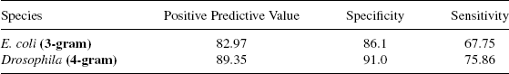
The results show that 3-grams are the best discriminators in E. coli, whereas, 4-grams are good in discriminating promoters from nonpromoters in Drosophila. It can be seen that the identification of nonpromoters being 85% is much higher than the promoter recognition results at 67%. The ratio of the positive-to-negative data sets is chosen to be 1:2. With the ratio of 1:1, the precision turns out to be 77.1%, specificity 75.69%, and sensitivity 80.47%. It can be seen that even though a much better recognition of promoters is achieved, false positives increase compared to the case when the training data set is in the ratio of 1:2. Hence, only the 1:2 case is used.
We had also experimented with random negative data sets that are obtained by generating nucleotide sequences randomly with 60 and 50% A+T composition used by some research groups [11]. Exceptionally good promoter classification results are obtained with precision, sensitivity, and specificity values being 95.5, 98.18 and 93.0%, respectively, with a single-layer perceptron [32]. Promoter classification with an accuracy of near 96% is achieved by a single-layer perceptron for synthetic negative data sets, potentially indicating the linear separability of the promoter data sets. But then these experiments cannot be used for the whole genome promoter prediction where the predictor has to annotate each nucleotide as belonging to a promoter or a nonpromoter based on the neighboring bases. Hence, it is important to carry on studies of promoter classification with nonpromoters obtained from the genome.
An indepth analysis is carried out in Section 4.3.3, to investigate the limitation on the sensitivity of promoter prediction using 3-gram features. A closer look at the misclassified promoter sequences showed that they belong to the reverse strand of the genome. This fact has to be further investigated.
In Section 4.3.3, we explore a global signal-based method that is based on FT and wavelet transform to extract features for the promoter recognition problem.
4.3.3 Investigation of Promoter Recognition in Frequency Domain
This section explores the application of signal processing techniques (e.g., Fast Fourier Transform (FFT) and wavelet transforms) for promoter recognition as well as the possibility of modeling the RNA polymerase–promoter interaction. Various encoding techniques [electron–ion interaction potential (EIIP), enthalpy, roll angle, etc.] are also included in the encoding of a sequence into a numerical format.
Tiwari et al. showned that the FT gene portion often has a prominent peak at 1/3 position confirming the periodicity of codons [34]. But, nongenes do not have any such peak. They have decomposed the original sequence into a set of four indicator sequences for the four nucleotides A, T, G, C [35]. Each sequence is a binary sequence indicating the presence or absence of a particular nucleotide. Deyneko et al. applied the physical features (e.g., melting enthalpy, roll angle, and minor groove depth of DNA) to find similar promoters that correlate with their transcription regulatory responsiveness to different antibiotic and osmotic treatments [36]. They transformed the E. coli promoters into numerical sequences using physical parameters (enthalpy, roll angle, etc.) Fourier Transform of the transformed sequences is used in computing cross-correlation and auto-correlation between different promoters. In particular, they looked for genes responsible for SOS response.
4.3.3.1 Encoding and Decomposition A DNA sequence is made up of four nucleotides A, T, G, and C. Different kinds of encodings have been used by different groups [37–39]. Nobuyuki et al. [37] used the values A = 1, T = -1, G = 1, and C = -1, whereas Cosic et al. [39] encoded the nucleotides by using the EIIP values: A: 0.1260, G: 0.0806, T: 0.1335, and C: 0.1340.
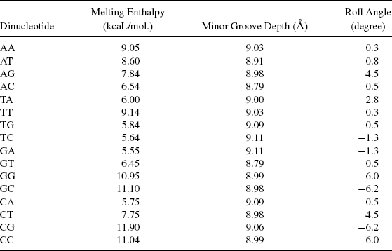
There are another set of encodings that are based upon dinucleotides. A large number of physicochemical parameters of DNA double strands/reflecting its specific properties have been collected in a public database [16]. Three parameter sets, melting enthalpy, minor groove depth, and roll, are given in Table 4.2. The DNA enthalpy data describes the melting of DNA double strands. The enthalpy data are dependent on the neighboring nucleotide and direction 5′ → 3′ is important here. The reason is that enthalpy is not only attributable to the direction invariant hydrogen bonds, but also to the interactions between electrons of neighboring bp. van der Waals forces also contribute to the interactions between the immediate base neighbors [40]. This information is not reversible for the strand direction and must therefore be taken into account in the enthalpy-based conversion of the primary structure into a signal [41]. Roll angle is another structural feature that may help in promoter recognition. A dinucleotide step is helically twisted since the distance between sugar–phosphate, backbone is twice the distance between base-stacking distance [42]. If a step is untwisted, the base pairs are pushed apart and the rise distance increases. To regain the stacking, (i.e., to decrease the rise distance) the step then rolls around the major groove [43]. For RNA polymerase to bind to the promoter, an open complex near the -10 site is required. Hence, this particular structural feature may be important in analyzing the dynamics of the DNA segment. The parameters are used to represent the DNA by Kauer and Co-workers [15,36]. Deyneko et al. [36] contend that the mere symbol computations are misleading since AA instead of GA numerically is more significant in terms of melting enthalpy. They claim that by using the physicochemical parameters, they were able to find significant similarity of promoters than with nucleotide comparison.
TABLE 4.2 Physicochemical Properties of DNA [36]
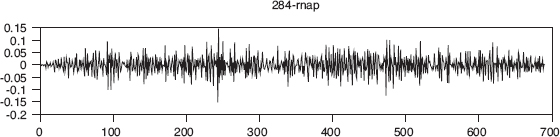
Here, we followed the EIIP encoding system of Cosic et al. for promoter–RNA polymerase interaction computations, since they also provide EIIP values for amino acids [39]. In the FT case, we used binary indicator sequences [35], enthalpy and roll angle encoding [36], and EIIP encoding [39]. Each sequence is encoded into a numerical sequence by using the encoding scheme. This numerical series is normalized to zero mean and unit standard deviation. Figure 4.2 depicts a sample sequence from the promoter data set that is converted into a numerical sequence using the EIIP values.
FIGURE 4.2 A sample promoter sequence represented in terms of EIIP values for nucleotides.

4.3.2.2 Feature Extraction Using one of these encodings, the original sequence is converted into a numerical series. This numerical series is transformed using FTs and WTs.
In FT, discrete fourier transform (DFT) is applied to the promoter, as well as nonpromoter sequences to cull out the dominant components in frequency space. Discrete FT is computed by using FFT in MATLAB. The FFT coefficients are complex, hence the power spectrum is computed using the FFT coefficients.
In wavelet transform, this series is decomposed using a discrete wavelet transform into a number of levels [44]. Bior3.3 biorthogonal wavelets are used to decompose the numerical promoter sequence.
As described earlier, a major portion of the data set is used for training the classifier and the rest that is not exposed to the classifier is used as the test data set. We denote the set of promoters as positive data set and the set of nonpromoters as the negative data set. Wavelet decomposition is done for each positive and negative sequence. This collection of vectors is divided into fivefolds in order to do the standard fivefold cross-validation. A neural network classifier is then trained using the wavelet feature vectors. The test set is used to evaluate the performance of the classifier.
In the case of a nonpromoter, data set consisting of both gene and inter-gene portions, the proportion of positive data set to the negative data set is taken as 1:2. Each promoter and nonpromoter sequence of the data set is encoded by using the coding scheme of Cosic et al [38]. Each sequence is decomposed into six levels by using Bior3.3. In total, there are 120 decomposition structure values that are required to decompose the original numerical sequence. The original wave is decomposed into six detail waves, namely, D1, D2, D3,D4, D5, D6, and one smooth component A6, each of length 80. The classification is based upon various features that are extracted from these decomposition structure values and decomposed wavelet coefficients.
4.3.3.3 Classification A multilayer feedforward neural network with three layers, namely, an input layer, one hidden and an output layer, is used for promoter classification in the following classification sections with various features based upon signal analysis techniques. The number of nodes in the input layer is dependent on particular features that are used. A hidden layer consists of a certain number of hidden nodes, the number found by trial and error that gives optimal classification performance. The output layer has one node to give a binary decision as to whether the given input sequence is a promoter or a nonpromoter. These simulations are done using Stuttgart neural network simulator [33].
Neural network is trained on the training set and then the classification performance is evaluated on the test set. All the classification experiments are carried out using a fivefold cross validation procedure [45,46]. The classification results are evaluated using performance measures (e.g., Precision, Specificity, and Sensitivity).
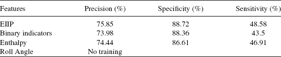
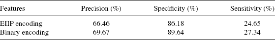
4.3.3.4 Classification Using Power Spectrum Features Earlier research using FT showed that the coding region of eukaryotes gave a peak at 1/3 pointing to a codon bias [34], which could be used in gene recognition in case of eukaryotes. In the case of prokaryotes, the periodicity of 3 is observed not only in coding regions, but also in noncoding regions [47]. If different triplets are responsible for periodicities in coding and noncoding regions, they may become helpful in identifying promoters and nonpromoters. Tiwari et al. [34] showed that the gene portion often has a prominent peak at 1/3 position confirming the periodicity of codons. But, nongenes do not have any such peak. They have decomposed the original sequence U into a set of four indicator sequences, namely, UA, UG, UT, and UC for the four nucleotides A, T, G, and C [34]. Each sequence is a binary sequence indicating the presence or absence of a particular nucleotide. Table 4.3 displays the classification results of E. coli with the power spectrum values as features for a feedforward neural network. The positive recognition results are not very encouraging even though negative recognition results are good, pointing possibly to the inseparability of coding versus noncoding sequences in this feature space.
TABLE 4.3 Classification Results Using Power Spectrum Values For E. coli Using Different Encoding Schemes
Experimenting with various lengths starting from 80 to 350 bp in steps of 40 bp for coding and noncoding sequences, we found that sequence lengths >200 bp might be needed to get a sizeable distinction near the 1/3rd peak. Hence, it is possible that the promoters versus nonpromoters are not able to throw up any distinct peak structure, which will be useful in classification of E.coli promoters.
In order to check the validity of the ideas, same experimentation is done on the Drosophila data set [23] used in Section 4.3.1. Here again the sequence is represented as a set of four binary-indicator sequences, each indicating the presence or absence of a particular nucleotide. Classification results using these encodings are shown in Table 4.4. The sensitivity is 50–60%, even though specificity is 85%. When the intron data is removed from the total data set, where is only consists of promoter and coding sequences, the sensitivity improves to 86%. Further, instead of binary values, if EIIP values are used in place of 1 in binary-indicator sequences, the sensitivity is much higher, ( 94%), which is supported by Trifonov and Sussman [47] data. Hence, it can be concluded that the intron part is similar to the promoter, which is hindering the classification accuracy. In view of the above arguments, in the case of E. coli, there are two factors that are affecting the accuracy: one is the length of the sequence and the second is the similarity of noncoding sequences to the promoter sequences. Thus FFT of the DNA sequence encoded using EIIP encoding, gives a slightly better accuracy compared to the other encodings for E. coli, and for Drosophila binary-indicator sequences gives a marginal improvement over EIIP encoding.
TABLE 4.4 Classification Results Using Power Spectrum Values for Drosophila Using Different Encoding Schemes
4.3.3.5 Classification Using Wavelet Coefficients A global signal using wavelet transforms is extracted from both promoter, as well as nonpromoter, sequences and is used as input to a classifier. Basically, there are two operations that can be performed on a signal: decomposition and reconstruction. One set of experiments is done using wavelet coefficients at various scales as features for a feedforward neural network to classify the promoter sequence. Another set of experiments is done using the decomposed waves as features to the classifier.
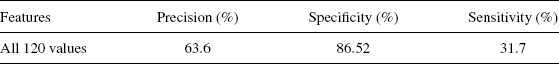
Simple FT is not enough to discriminate a promoter against coding and noncoding backgrounds as seen above. The time or positional information is lost in an FT. Wavelet transform retains the positional, as well as frequency information. The decomposition structure has a total number of coefficients of 120. The values are 8, 8, 9, 11, 16, 25, and 43 for A6, D6, D5, D4, D3, D2, and D6, respectively. The classification accuracy of promoter recognition problem is computed using wavelet coefficients as input to the neural network. The results are given in Table 4.5. The results show that nonpromoter recognition is good compared to promoter recognition.
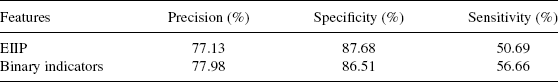
TABLE 4.5 Classification Results Using Wavelet Coefficients as Features for a Neural Network Classifier for E. coli Using EIIP Encoding
4.3.3.6 Classification Using Decomposed Signals Each decomposed wave is rebuilt using decomposed structure values into a wave of length 80. In total, there are seven waves, namely, A6, D6, D5, D4, D3, D2, and D1 resulting in 560 values (7 × 80). All waves are used to see whether more information is imparted by transforming one initial signal wave into so many decomposed waves. These 560 values are used as input features to a neural network classifier to identify the promoters. Table ef{Table:waves} presents the results of the classifier for these feature values. The results again are showing good nonpromoter recognition rather than promoter recognition. It can be concluded that both experiments using wavelet coefficients and decomposed waves are good for nonpromoter recognition. Increase in the number of features has not helped in gaining more information to classify promoters better. Experiments on the Drosophila data set also present similar results. The sensitivity is 50% for Drosophila using binary indicator sequence encoding scheme. The results are shown in Table 4.7.
TABLE 4.6 Classification Results Using Decomposed Waves as Features to a Neural Network Classifier for E. coli Using EIIP Encoding
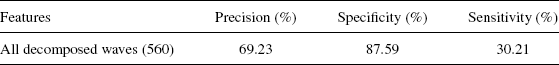
TABLE 4.7 Classification Results Using Decomposed Waves as Features to a Neural Network Classifier for Drosophila Binary Indicators Encoding Scheme
4.3.3.7 Cross-Correlation between Promoter and RNA-Polymerase We also looked at modeling the interaction between promoter and RNA polymerase during promoter recognition [48]. Basically, interactions between protein and DNA can be categorized into four classes: DNA backbone–protein backbone (18%), DNA backbone–protein side chain (51%), DNA side chain–protein backbone (1%) DNA side chain–protein side chain (30%) [49]. Protein–DNA interactions are chemically the same as protein–protein interactions. They consist of electrostatic interactions, hydrogen bonds, and hydrophobic interaction. However, hydrogen bonds constitute the major term for recognition and specificity and a large portion of the binding energy [50,51]. It has been proposed that matching of periodicities within the distribution of energies of free electrons along the interacting proteins or protein and DNA can be regarded as resonant recognition [38]. The whole process can be observed as the interaction between transmitting and receiving antennaes of a radio system.
The sigma subunit of the RNA polymerase is of 612 aa (amino acids) length. The subunit is converted into a numerical sequence using the EIIP values for the aa [44]. This particular subunit is also decomposed into six levels using the Bior3.3 biorthogonal wavelet. The maximum absolute value of the correlation coefficient at each decomposition level can be treated as the similarity score between the signals. Cross-correlation between RNA polymerase and sample sequence is given Figure 4.3. The number of correlation coefficients is 691. In case of binary encoding, wavelet at a particular level is obtained by taking the norm of four vectors for each i,j where i is the location and j is the level number as
FIGURE 4.3 Cross-correlation between sample promoter and RNA polymerase subunit sigma.
The results of classification using both these encodings are given in Table 4.8.
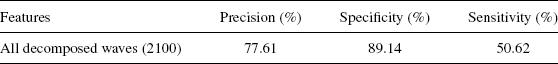
TABLE 4.8 Classification Results Using DNA–RNA Polymerase Sigma Subunit Cross-Correlation Values as Features for a Neural Network Classifier for E. coli
The results using features of cross-correlation between promoter and RNA polymerase sigma subunit, and cross-correlation between decomposed waves of both promoter and RNA polymerase sigma subunit have shown a remarkable ability to identify nonpromoters. Finally, the assumption that signal processing methods can capture the interaction between the RNA polymerase sigma subunit and promoter has not fructified well. It is also found that the different encoding schemes, including those that use the structural properties of the genome do not influence the classification performance.
4.4 CHALLENGES IN PROMOTER CLASSIFICATION
4.4.1 Limitations in the Neural Network Performance
Detailed analysis of the classification results of promoters of E. coli is carried out with the best features, which are 3-grams as basis. Many experiments are carried out in the training phase of the neural network by varying the network architecture with different number of hidden layers and the number hidden nodes in each hidden layer. Yet, the network could not achieve a training performance beyond 85%. The sets of misclassified and correctly classified sequences are studied closely by keeping the feature extraction and the classifier scheme as described in Sections 4.3.2.1 and 4.3.2.2. For a deeper analysis of promoters classification, a set of sequences is selected randomly from both promoters and nonpromoters (consisting of both gene and intergene portions) in the ratio of 1:2, respectively, for training. That is, a set of 454 sequences are taken from a promoter data set as a positive set, and 454 sequences are taken from each gene and inter-gene sequence sets. The rest of the data set is used as a test data set.
It clearly can be seen from Figure 4.4 and Table 4.9 that the true positives and false positives stay together and the true negatives and the false negatives are not distinguishable in this feature space.
FIGURE 4.4 Plot of 3-gram frequency averages for promoter and negative data sets consisting of segments from gene and inter-gene portions of the DNA.
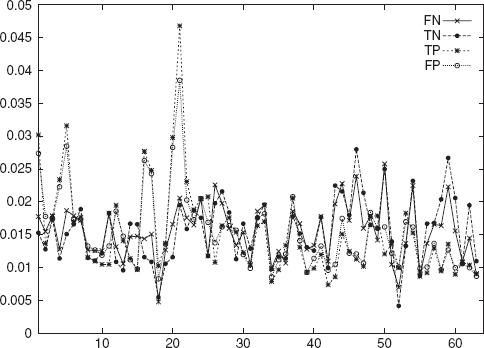
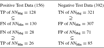
The experiments clearly demonstrate that there is a small confusion set in both the promoter and nonpromoter data sets. We categorize the two classes within the data set as the “majority” promoter–nonpromoter class and the other that reflects the “minority” signal. Now, the sequences that the neural network finds difficult to classify are isolated from both positive and negative data sets. In the following experiment, we reconstitute the data set by removing the minority data set from both the promoter and nonpromoter sets and call it Major Set (Maj). It is found that a neural network, which we call NNMaj, without a hidden layer achieves 100% training performance and the results of the test data set are shown in Table 4.10.
TABLE 4.9 Test Data Results of Neural Networks NNMaj and NNMin
Similar performance is observed for the neural network NNMin when trained only on Min. That is, the Maj class constituting the majority promoter and the majority nonpromoters is linearly separable. Similarly, the Min set is also linearly separable.
Note that in Table 4.9 the numbers as well as the exact sequences in each of these boxes match. For example, the set of 130 FNs of NNMin is a superset of the 128 TPs of NNMaj. Thus, we see that both promoter and nonpromoter sequences have two distinct patterns, one being recognized by NNMaj and the other by NNMin. But for 5–7 sequences, the NNMaj and NNMin behave in a complementary fashion, which is confusing. A small portion (14%) of the nonpromoter data set is similar to a majority (70%) of the promoter data set. Also, 86% of the nonpromoter data set (TN) is closer to 30% of the promoter data set (FN).
When the misclassified sequences are removed, it is clear that the classification results will be very good, but it is surprising that a single-layer perceptron is able to achieve accuracy when the confusion set is removed. Note that in this process we have successfully built a neural network NNMaj, which is a single-layer perceptron achieving promoter recognition performance of 80%. This result is comparable to the powerful classifiers that are presented in the literature [22].
TABLE 4.10 Classification Results of NNMaj a Single Layer Perceptron
4.4.2 Genome-Wide Promoter Recognition
A main goal of promoter recognition is to locate promoter regions in the genome sequence. In this section, a scheme for locating promoters in a given DNA sequence segment of E. coli genome of length N in a particular direction (say, 5′–3′) is proposed. The scheme does not address the issue of locating TSS in the promoter region. The NNMaj network is a classifier that is constructed with the negative data set composed of genic and intergenic portions. When the negative data set is a combination of both coding and noncoding segments, it is advantageous in the sense that the promoter and nonpromoter could be classified at the same time. But, the classification accuracy is not 100%, and there is no way one can eliminate the false positives and negatives. To overcome this handicap, instead of using the earlier neural networks, a new set of neural networks based on different combinations of the data sets are designed. One network, NNPC, is trained using promoter and coding data sets as positive and negative data sets, respectively, and another one, NNPN, using promoter and noncoding data sets.
A moving window of length 80 is considered to extract segments from the start of the DNA sequence, that is, 1–80, 2–81, 3–82, and so on. A given sequence segment is classified as promoter by a voting scheme. If NNPC and NNPN both classify the sequence as a promoter sequence, then the sequence is voted as a promoter or otherwise a nonpromoter. Each of the segments thus gets classified as a promoter (P) or nonpromoter (NP). If a segment m-(m+79) is classified as a promoter, then the nucleotide m is annotated as P and if it is classified as nonpromoter, then m is annotated as NP. This process of annotation is continued for the entire sequence to get a sequence of P’s and NPs. A stretch of these outcomes greater than a threshold (e.g., 50 consecutive positive outcomes) is treated as a P or as an NP region.
The whole genome of E. coli is divided into 400 sections. The following is a case study on two sections (Sections 1 and 3) of E. coli whole genome. The combined outputs of NNPC and NNPN, as described earlier, is used to annotate the promoter regions. The consensus regions can be seen in Figures 4.5 and 4.6. Since NNPN shows many spurious promoters, it is essential to take the consensus result. In the figures, the output result of the ensemble of networks of NNPC and NNPN is shown to indicate that a consensus for a stretch of >50 bp will be annotated as a promoter.
FIGURE 4.5 The combined output of the networks NNPC and NNPN versus the moving window for section1 of the E. coli genome.
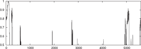
FIGURE 4.6 The combined output of the networks NNPC and NNPN versus the moving window for section3 of the E. coli genome.
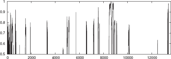
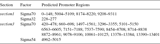
Table 4.11 shows the section number, the sigma factor, and the extent of the region identified as promoter from the experiment. In the whole genome annotation, it is considered essential that no true promoter is missed. The n-gram based classifier is able to annotate all the existing promoters that are in NCBI in the sections that are considered. On the other hand, a few regions are additionally annotated as promoters. For example in section3, 3296–3355, 7537–7590, 8454–8708 which are regions predicted as promoters, are not accounted for in the NCBI data. Only wet lab experiments can verify the validity of this result.
TABLE 4.11 Promoter Regions Predicted by the Neural Networks NNPC and NNPN
There are not many whole genome promoter prediction programs for prokaryotes. The available tools for prokaryotic promoter prediction are that of Gordon et al.[52] who developed a whole genome promoter prediction based on their sequence alignment kernel (SAK); Bacterial Promoter BPROM is developed by SoftBerry Inc. [53]; Neural network promoter prediction (NNPP) tool developed by Reese [54]. SAK predicts whether the 61st position of a sequence of length 80 is a TSS or not. The legend of SAK says that the more positive the outcome is, the more probable that segment is a promoter, and a promoter, is denoted by “L”. There are no such annotations in the test case. But, it can be seen that most of the peaks coincide. In the case of BPROM, an internal parameter threshold for promoters is set as 0.20 [51]. Bacterial promoter (BPROM) has predicted 31 promoters in this region. Further, BPROM predicts the TSS and determines the binding regions. The NNPP predictions are made with a cut-off rate of 0.80 [55]. A comparative study of promoter recognition by these tools along with 3-grams shows that 3-grams outperform these tools. Classifier based on 3-grams achieves 100% sensitivity, whereas SAK, NNPP, and BPROM achieve 69.23, 76.92, and 38.46, respectively.
The results give a clear indication that cascaded networks based on 3-grams perform significantly well. One more factor is that, unless we know, here a promoter region exists, we cannot say an outcome from these other tools is positive since there are many false positives. In our scheme, wherever we find a stretch of positives, using the cascaded method, we can label them as positive predictions.
The promoter prediction is carried out for the Drosophila genome with the ensemble of neural networks of NNPC and NNPN using 4-grams. A stretch of 10 kbp is used that starts with a gene followed by two more genes. For this data, four promoters are identified by the ensemble of which two promoters occur before the genes and one in the intron region and one in the exon region. The stretches of promoter occurring in intron and exon portions are 150 bp in length, whereas the portions identified before the genes are 350 bp in length. The threshold has to be set more rigorously, by more experimentation. The NNPP2.2 is used for cross-checking the method as the data set for Drosophila is taken from them. The NNPP2.2 software predicted 21 promoters with a cutoff of 0.8, 8 with a cutoff of 0.95 and only one with a cutoff of 0.99. In this, the cutoff plays a crucial role. The other software package FirstEF did not predict any promoter at all.
4.5 CONCLUSIONS
In the literature, the techniques proposed for feature extraction can be broadly classified as those that exploit biological information explicitly and those that do not need a priori biologically based labeling information. In the former category, called the local methods, the features are extracted from the binding regions or local motifs, whereas in the latter, global signal methods, features are derived utilizing the physicochemical and structural properties of the whole promoter region. The recognition methods that exploit the promoter signal like the position weight matrices (PWM), the expectation maximization algorithm, and the techniques like FTs, are proposed in the literature. This chapter presents promoter recognition using n-gram based features and features based on FT and WT. We demonstrate that the n-gram based features perform the best for the whole genome annotation.
Whole genome annotation is a major challenge for promoter prediction tools. The performance of an algorithm on a limited training and test data set may not be really a performance indicator of how well it may identify promoters in a whole genome. Methods that are proposed giving good accuracies on training and test data sets, may or may not perform better on the whole genome.
The binding regions are important in assisting the RNA polymerase to bind the promoter, but that information alone is not sufficient to recognize a promoter. Local features are calculated from binding sites that are available in Harley’s data cite{Harley}. Global features are extracted from the whole promoter sequence aligned with respect to TSS and nonpromoter data sets.
If we compare the results that are obtained using a signal extracted from motifs–binding regions in the promoter with the signal obtained from the whole promoter sequence, it is evident that the local signal has a handicap in extending to a whole genome promoter prediction process. The signal from the entire promoter sequence without segmenting it into important and nonimportant portions will lead to better generalization in the case of E. coli. The PWM based features, as well as n-grams from the whole promoter, give better genome promoter annotation results than the other local signal extraction schemes.
Experiments are carried out to find a signature of the promoter present at any particular resolution. If the characteristic signal of a promoter that is supposed to be conserved irrespective of place of occurrence of the genome promoter is not preserved, then promoter recognition based on the signal processing techniques will not be very helpful. The results of E. coli and Drosophila show that features using FFT and wavelets are not sufficient to recognize a promoter against a coding and noncoding background. This fact is evident from the results where the negative data seems to be recognized better than a promoter. The promoter data set seems to have no pattern in the FT, WT feature space that can be learned by the classifier. In summary, it turns out that signal processing techniques cannot be used as general classification algorithm. The conjecture that structural properties are underlying principles for base selection is not evident from the current experiments.
This chapter shows that in an n-gram feature space, recognition rate of Drosophila promoters is better than E. coli promoter recognition. Best performance for Drosophila is 87% compared to E. coli’s 80% with a very good positive predictive rate as shown in Section 4.3.2.2. Promoter architecture of eukaryotes is in general much more complex than a prokaryote promoter architecture. It is found that n-gram preferences for Drosophila is stronger in a discriminating promoter versus a nonpromoter than for E. coli. The prediction of the negative data set is higher possibly because the intron portions are similar to nongene segments in eukaryotes. In fact, the results of promoter recognition using FT give only ∼50% positive identification.
From these results, we can conclude that different adjacency preferences are shown for promoter and nonpromoter regions. One major advantage of using n-gram based whole genome promoter annotation is that one does not need any prior information about the promoter, the location of binding sites, the spacer lengths, and so on. The additional advantage of using n-gram features is that the input vectors computed for neural network classifier will not change irrespective of the length of the promoter sequence.
4.6 FUTURE DIRECTIONS
The techniques described in this chapter can be developed to build a full-fledged automated whole genome promoter annotation tool. Whole genome promoter prediction using 3-grams has been applied to the forward strand only. The same scheme needs to be applied to the reverse strand with appropriate preprocessing so that the method can achieve whole genome promoter recognition.
Signal processing techniques need to be explored further to enhance the recognition rates. Since RNA polymerase is an enzyme, which is a protein, three-dimensional structure information of RNA polymerase can be used to characterize promoter–RNA polymerase interaction. It is to be explored if instead of using Bior3.3 as the mother wavelet, RNA polymerase itself can be used as a mother wavelet to imitate the biological mechanism closely. This line of application of wavelets would be quite novel.
Proteins are believed to be responsible for most of the genetically important functions in all cells. Hence, the focus has been entirely on gene recognition. Recent studies indicate that ncRNAs (noncoding RNAs), which do not code for proteins, affect transcription and the chromosome structure, in RNA processing and modification, regulation of mRNA stability and translation, and also affect protein stability and transport [56,57]. An effort to look for them in typically 95% of the total DNA is a huge task. By suitably modeling the promoters of these ncRNAs, they can be predicted much more easily. Some of the techniques that are developed here can be extended to do this work.
REFERENCES
1. R. Grosschedl and M. L. Birnstiel (1980), Identification of regulatory sequences in the prelude sequences of an h2a histone gene by the study of specific deletion mutants in vivo, Proc. Natl. Acad. Sci., 77(12): 7102–7106.
2. S. L. McKnight and K. R. Yamamoto (1992), Transcriptional regulation, Cold Spring Harbor Laboratory Press, MA.
3. FANTOM Consortium (2005), RIKEN Genome Exploration Research Group and Genome Science Group (Genome Network Project Core Group), The transcriptional landscape of the mammalian genome Science, 309: 1559–1563.
4. V. G. Levitsky and A. V. Katokhin (2003), Recognition of eukaryotic promoters using a genetic algorithm based on iterative discriminant analysis, In Silico Biol. 3.
5. A. G. Pedersen, P. Baldi, Y. Chauvinb, and S. Brunak (1999), The biology of eukaryotic promoter prediction—a review, Comput. Chem., 23: 191–207.
6. V. B. Bajic, S. H. Seah, A. Chong, G. Zhang, J. L. Y. Koh, and V. Brusic (2002), Dragon promoter finder: recognition of vertebrate RNA polymerase II promoters, Bioinformatics, 18(1): 198–199.
7. J. M. Claverie and S. Audic (1996), The statistical significance of nucleotide position-weight matrix matches, CABIOS, 12(5): 431–439.
8. N. I. Gershenzon, G. D. Stormo, and I. P. Ioshikhes (2005), Computational technique for improvement of the position-weight matrices for the DNA/protein binding sites, Nucleic Acids Res., 33(7): 2290–2301.
9. S. W. Leung, C. Mellish, and D. Robertson (2001), Basic gene grammars and DNA-chart parser for language processing of Escherichia coli promoter DNA sequences, Bioinformatics, 17: 226–236.
10. L. R. Cardon and G. D. Stormo (1992), Expectation maximization algorithm of identifying protein-binding sites with variable lengths from unaligned DNA fragments, J. Mol. Biol., 223: 159–170.
11. Q. Ma, J. T. L. Wang, D. Shasha, and C. H. Wu (2001), Dna sequence classification via an expectation maximization algorithm and neural networks: a case study, IEEE Transactions on Systems,Man and Cybernetics, Part C:
12. Applications and Reviews, Special Issue on Knowledge Management, 31: 468–475.
13. T. Werner (1999), Models for prediction and recognition of eukaryotic promoters, Mammalian Genome, 10: 168–175.
14. M. K. Das and H. K. Dai (2007), A survey of DNA motif finding algorithms, BMC Bioinformat., 8: (7:S21).
15. A. M. Huerta and J. Collado-Vides (2003), Sigma70 promoters in escherichia coli: Specific transcription in dense regions of overlapping promoter-like signals, J. Mol. Biol., 333: 261–278.
16. G. Kauer and B. Helmut (2003), Applying signal theory to the analysis of biomolecules, Bioinformatics, 19(16): 2016–2021.
17. J. V. Ponomarenko, M. P. Ponomarenko, A. S. Frolov, D. G. Vorobyev, G. C. Overton, and N. A. Kolchanov (1999), Conformational and physicochemical DNA features specific for transcription factor binding sites, Bioinformatics, 15: 654–668.
18. F. Kobe, S. Yvan, D. Sven, R. Pierre, and Y. P. Peer (2005), Large-scale structural analysis of the core promoter in mammalian and plant genomes, Nucleic Acids Res., 33(13): 4255–4264. W. Li (1997), The study of correlation structures of DNA sequences: a critical review, Comp. Chem., 21: 257–271.
19. C. B. Harley and R. P. Reynolds (1987), Analysis of e.coli promoter sequences, Nucleic Acids Res., 15(5): 2343–2361.
20. L. Pietro (2003), Wavelets in bioinformatics and computational biology: state of art and perspectives, Bioinformatics, 19(1): 2–9.
21. J. D. Alicia, D. J. Bradley, L. Michael, and A. G. Carol (1996), The sigma subunit of escherichia coli RNA polymerase senses promoter spacing, Proc. Nat. Acad. Sci., 93: 8858–8862.
22. L. Gordon, A. Y. Chervonenkis, A. J. Gammerman, I. A. Shahmurradov, and V. Solovyev (2003), Sequence alignment kernel for recognition of promoter regions, Bioinformatics, 19: 1964–1971.
23. U. Ohler, G. C. Liao, H. Niemann, and G. M. Rubin (2002), Computational analysis of core promoters in the drosophila genome, Genome Biology 2002, 3(12):research0087.1-0087.12.
24. Eukaryotic Promoter Database (EPD). Available at http://www.epd.isb-sib.ch/index.html
25. I. Ben-Gal, A. Shani, A. Gohr, J. Grau, S. Arviv, A. Shmilovici, S. Posch, and I. Grosse (2005), Identification of transcription factor binding sites with variable-order Bayesian networks, Bioinformatics, 21; 2657–2666.
26. F. Leu, N. Lo, and L. Yang (2005), Predicting vertebrate promoters with homogeneous cluster computing, In Proc. 1st International Conference on Signal-Image Technology and Internet-Based Systems (SITIS), pp. 143–148.
27. H. Ji, D. Xinbin and Z. Xuechun (2006). A systematic computational approach for transcription factor target gene prediction, in IEEE Symposium on Computational Intelligence and Bioinformatics and Computational Biology CIBCB ‘06, pp. 1–7.
28. J. Wang and S. Hannenhalli (2006), A mammalian promoter model links cis elements to genetic networks, Biochem. Biophys. Res. Commun. 347: 166–177.
29. Q. Z. Li and H. Lin (2006), The recognition and prediction of σ70 promoters in Escherichia coli K-12, J. Theor. Biol., 242: 135–141.
30. S. Sonnenburg, A. Zien, P. Philips, and G. Ratsch (2008), POIMs: positional oligomer importance matrices—understanding support vector machine—based signal detectors, Bioinformatics, 24: i6–i14.
31. T. Sobha Rani and Raju S. Bapi (2008), Analysis of n-gram based promoter recognition methods and application to whole genome promoter prediction, In Silico Biol., 9: s1–s16.
32. T. S. Rani, S. D. Bhavani, and R. S. Bapi (2007), Analysis of E. coli promoter recognition problem in dinucleotide feature space, Bioinformatics, 23: 582–588.
33. Stuttgart Neural Network Simulator. Available at http://www-ra.informatik.uni-tuebingen.de/SNNS/
34. S. Tiwari, S. Ramachandran, A. Bhattacharya, S. Bhattacharya, and R. Ramaswamy (1997), Prediction of probable genes by fourier analysis of genomic sequences, Comput. Appl. Biosci., 13: 263–270.
35. R. F. Voss (1992), Evolution of long-range fractal correlations and 1/f noise in DNA base sequences, Phys. Rev. Lett., 68(5): 3805–3808.
36. I. V. Deyneko, E. K. Alexander, B. Helmut, and G. Kauer (2005), Signal-theoretical DNA similarity measure revealing unexpected similarities of E. coli promoters, In Silico Biol., 5.
37. K. Nobuyuki, O. Yashurio, M. Kazuo, M. Kenichi, K. Jun, C. Piero, H. Yoshihide, and K. Shoshi (2002), Wavelet profiles: Their application in Oryza Sativa DNA sequence analysis, In Proc. IEEE computer society Bioinformatics conference(CSB02), pp. 345–348.
38. A. Arneodo, E. Bacry, P. V. Graves, and F. Muzy (1995), Characterizing long-range correlations in DNA sequences from wavelet analysis, Phys. Rev. Lett., 74(16): 3293–3297.
39. I. Cosic (1994), Macromolecular bioactivity( is it resonant interaction between macromolecules?-theory and applications, IEEE Trans. Biomed. Eng., 41(12): 1101–1114.
40. M. Suzuki, N. Yagi, and J. T. Finch (1996), Role of base-backbone and base-base interactions in alternating DNA conformations, FEBS Lett., 379: 148–152.
41. T. V. Chalikian, J. Volkner, G. E. Plum, and K. J. Breslauer (1999), A more unified picture for the thermodynamics of nucleic acid duplex melting: A characterization by calorimetric and volumetric techniques, Proc. Natl. Acad. of Sci. USA, 96: 7853–7858.
42. C. R. Calladine and D. R. Drew 1992, Molecular Structure and Life, CRC Press.
43. A. A. Gorin, V. B. Zhurkin, and W. K. Olson (1995), B-DNA twisting approach correlates with base-pair morphology, J. Mol. Biol., 247: 34–48.
44. H. T. Chafia, F. Qian, and I. Cosic (2002), Protein sequence comparison based on the wavelet transform approach, Protein Eng., 15(3): 193–203.
45. E. Alpaydin (2004), Introduction to Machine Learning, MIT Press.
46. T. M. Mitchell, Machine Learning, McGraw Hill, Singapore, 1997.
47. E. N. Trifonov and J. L. Sussman (1980), The pitch of chromatin DNA is reflected in its nucleotide sequence, Proc. Natl. Acad. Sci. USA 77: 3816–3820.
48. T. Sobha Rani and Raju S. Bapi (2008), E. coli Promoter Recognition Through Wavelets, Proc. BIOCOMP 2008, 256–262.
49. Y. Mandel-Gutfreund, O. Schueler, and H. Margalit (1995), Comprehensive analysis of hydrogen bonds in regulatory protein DNA-complexes: In search of common principles, J. Mol. Biol., 253: 370–382.
50. N. M. Luscombe, R. A. Laskowski, and J. M. Thornton (2001), Amino-acid base interactions a three-dimensional analysis of protein-DNA interactions at atomic level, Nucleic Acids Res., 29: 2860–2874.
51. K. Luger, A. W. Mader, R. K. Richmond, D. F. Sargent, and T. J. Richmond (1997), Crystal structure of the nucleosome core particle at 2.8 a resolution, Nature (London), 389: 251–260.
52. Sequence Alignment Kernel. Available at http://nostradamus.cs.rhul.ac.uk/leo/sak_demo.
53. Prediction of Bacterial promoters (BPROM). Available at http://www.softberry.com/berry.phtml?topic =bprom
54. Berkeley Drosophila Genome Project (BDGP). Available at http://www.fruitfly.org/seq_tools/promoter.html
55. Neural Network Promoter Predictor (NNPP). Available at http://www.fruitfly.org/seq_ tools/promoter.html
56. J. S. Mattick (2003), Challenging the dogma: the hidden layer of non-protein-coding RNAs in complex organisms, BioEssays, 25: 930–939.
57. S. Gisela (2002), An expanding universe of noncoding rnas, Science, 296: 1260–1263.