
CHAPTER 7
KERNELS ON PROTEIN STRUCTURES
7.1 INTRODUCTION
Kernel methods have emerged as one of the most powerful techniques for supervised, as well as semisupervised learning [1], and with structured data. Kernels have been designed on various types of structured data including sets [2–4], strings [5], probability models [7,8], and so on. Protein structures are another important type of structured data [9,10], which can be modelled as geometric structures or pointsets [9,10]. This chapter concentrates on designing kernels on protein structures [7,11].
Classification of protein structures into different structural classes is a problem of fundamental interest in computational biology. Many hierarchical structural classification databases, describing various levels of structural similarities, have been developed. Two of the most popular databases are structural classification of proteins (SCOP) [12] a manually curated database, and class, architecture, topology and homologous superfamilies (CATH) [13], which is a semiautomatically curated database. Since the defining characteristics of each of these classes is not known precisely, machine learning is the tool of choice for attempting to classify proteins automatically. We propose to use the kernels designed here along with support vector machines to design automatic classifiers on protein structures.
Many kernels have been designed to capture similarities between protein sequences. Some of the notable ones include Fisher kernels [6], kernels based on comparison of k-mers [5], and alignment kernels [15]. However, the problem of designing kernels on protein structures remains relatively unexplored. Some of the initial attempts include application of graph kernels [15] and empirical kernel maps with existing protein structure comparison algorithms [16]. Reference [17] defines various kernels on substructures using amino acid similarity. However, they fail to capture structural similarity in a principled way. These kernels are used mainly for finding structural motifs and annotating functions.
In a recent paper [18], we proposed several novel kernels on protein structures by defining kernels on neighborhoods using ideas from convolution kernels [19]. These kernels captured the shape similarity between neighborhoods by matching pairwise distances between the constituent atoms. This idea of using only geometric properties to find similarity between proteins is also adopted by many protein structure comparison algorithms [8,11]. We also generalized some of these kernels to attributed pointsets [10], and demonstrated their application to various tasks in computer vision.
This chapter reports a detailed exploration of the idea of defining kernels on protein structures using kernels on neighborhoods, which are specific types of substructures. The idea of neighborhoods has been used previously to design protein structure comparison algorithms [11], which performed competitively with the state of the art. Kernels on neighborhoods are subdivided into two types: those using sequence or structure information. Sequence-based kernels on neighborhoods draw ideas from the general set kernels designed in [4] and convolution kernels [19]. Structure-based kernels are motivated from protein structure comparison algorithms using spectral graph matching [11,20]. We show that in a limiting case, the kernel values are related to the similarity score given by protein structure comparison algorithms.
We also explore two different ways of combining sequence- and structure-based kernels, weighting and convex combination, to get kernels on neighborhoods. Finally, we explore two methods of combining the neighborhood kernels, one without using structural alignment, and the other using structural alignment. Interestingly, even though spectrum kernels [5] were defined using feature spaces involving k-mers, we show that they are a special case of our kernels when using only sequence information on sequence neighborhoods.
Extensive experimentation was done to validate the kernels developed here on real protein structures and also to study the properties of various types of kernels. The task chosen was that of classifying 40% sequence nonredundant SCOP [12] superfamilies, which was also demonstrated to be very difficult and relevant. Our kernels outperformed the state of the art protein structure comparison algorithm combinatorial extension (CE) [21]. We also compared our kernels with spectrum kernels [5] and experimentally validated a theoretical property of the structure-based neighborhood kernels.
This chapter is organized as follows: Section 7.2 gives a background of kernel methods and various kernels on structured data. Section 7.3 gives a background on protein structures, describes the protein-structure alignment problem and develops a neighborhood-based algorithm for protein-structure alignment, which is a simplified version of the formulation used in [11]. Section 7.4 proposes kernels for sequence and structure neighborhoods. Section 7.5 defines various kernels on protein structures using the neighborhood kernels defined in Section 7.4. Section 7.6 describes the experimental results obtained with various kernels proposed here and also compares them to existing techniques. We conclude with remarks in Section 7.7.
7.2 KERNELS METHODS
Kernel methods [1,22,23] is the collective name for the class of learning algorithms that can operate using only a real valued similarity function (called kernel function) defined for each pair of datapoints. Kernel methods have become popular over the last decade, mainly due to their general applicability and theoretical underpinnings.
A critical step in the effectiveness of a kernel method is the design of an appropriate kernel function. A function ![]() , is called a positive semidefinite or Mercer kernel if it satisfies the following properties:
, is called a positive semidefinite or Mercer kernel if it satisfies the following properties:
A positive semidefinite kernel K maps points x,y![]() X to a reproducing kernel Hilbert space (RKHS)
X to a reproducing kernel Hilbert space (RKHS) ![]() be the corresponding points, the inner product is given by:
be the corresponding points, the inner product is given by:
Also, for a finite dataset ![]() , the n× n kernel matrix Kij= K(xi,xj), constructed from a positive semidefinite kernel K, can decomposed using eigenvalue decomposition as:
, the n× n kernel matrix Kij= K(xi,xj), constructed from a positive semidefinite kernel K, can decomposed using eigenvalue decomposition as:
Thus, the feature map ψx can be explicitly constructed as
This effectively embeds the points into a vector space, thus allowing all the vector space-based learning techniques to be applied to points from the arbitrary set X. Some of the common methods to be kernelized are support vector machines, principal component analysis, Gaussian process, and so on (see [1] for details).
7.2.1 Kernels on Structured Data
It is clear from the above discussion that definition of the kernel function is the key challenge in designing a kernel method. This section enumerates some of the well-known kernels that are related to the work described here. We begin by describing operations under which the class of positive semidefinite kernels is closed.
If K is a positive semidefinite (PSD) kernel, so is α K for α > 0.
If K1 and K2 are PSD kernels, so are K1 + K2 and K1 K2.
If Kn, n = 1,2, … are PSD kernels and K = limn→ ∞ Kn exists, K is a PSD kernel.
If K1 is a PSD kernel on X ×X and K2 is a PSD kernel on Z × Z, then the tensor product K1⊗ K2 and the direct sum K1⊕ K2 are PSD kernels on X × Z× X ×Z.
For proofs of these closure properties, please see [1,22,23]. From the above properties, it can also be shown that ![]() is a PSD kernel if K is a PSD kernel.
is a PSD kernel if K is a PSD kernel.
Intuitively, kernels between arbitrary objects can be thought of as similarity measures. To see this, recall that the inner product ![]() defined by kernel function K induces a norm
defined by kernel function K induces a norm ![]() in the RKHS H. This norm induces a natural distance metric, defined as
in the RKHS H. This norm induces a natural distance metric, defined as ![]() . It is easy to see that
. It is easy to see that
Thus, d(x,y) is a decreasing function of K(x,y). So, K(x,y) can be thought of as a similarity function.
Various kernels between vectors have been used in the literature. Most simple of them is the dot product or linear kernel, given by
This kernel uses an identity feature map. Another popularly used kernel between vectors is the Gaussian kernel:
It is useful when one simply wants the kernel to be a decreasing function of the Euclidean distance between the vectors.
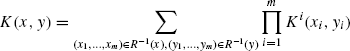
One of the most general types of kernels on structured data are the convolution kernels [19]. Convolution kernels provide a method of defining PSD kernel on composite objects using kernels on parts. Let X be a set of composite objects consisting of parts from X1,…,Xm. Let R be a relation over ![]() , such that
, such that ![]() is composed of x1, …,xm. Also, let
is composed of x1, …,xm. Also, let ![]() and Ki be kernels on Xi ×Xi. The convolution kernel K on X × X is defined as
and Ki be kernels on Xi ×Xi. The convolution kernel K on X × X is defined as
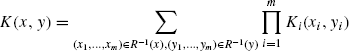
It can be shown that if K1,…,Km are PSD, then so is K. Convolution kernels have been used to iteratively define kernels on strings [14,19], and applied to processing of biological sequences. They have also been used in natural language processing for defining kernels on parse trees [24]. We use convolution kernels to define kernels on neighborhoods.
Kernels on sets of vectors are the next most general types of kernels and have also been useful in designing kernels for protein structures. It was shown in [25] that given two d × c matrices X and Y:
are PSD kernels. Both [2] and [25] define kernels on the subspaces spanned by set of vectors. They show that if UX and UY are orthogonal matrices spanning column spaces of X and Y, then the product of cosines of principal angles between the column spaces is given by
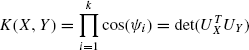
where ψi are the principal angles. This kernel was applied to problems in computer vision [2] (e.g., detection of abnormal motion trajectories and face recognition). These kernels are further generalized in [25]. Shashua et al. also define a general class of kernels on matrices [4]. They show that given two matrices An× k and Bn× q:
is a PSD kernel where, zero extensions of ![]() and
and ![]() Fr and Gr, are such that ∑r Fr ⊗ Gr is PSD.
Fr and Gr, are such that ∑r Fr ⊗ Gr is PSD.
Strings are a type of structured data that find wide applicability in various fields, including biological sequence analysis, text mining, and so on. While the kernels described above can and have been used for string processing, rational kernels, defined in [26] are a general class of kernels defined specifically for strings. Cortes et al. [26] give a general definition of rational kernels and show various theoretical results on conditions for rational kernels to be PSD. A popular special case of these kernels are the k-mer based kernels defined in [5]. Let Σ be the alphabet from which the string is generated, the feature map, ψ, for the kernels are defined by |Σ|k dimensional vector indexed by all k-mers. The value of ψi(x) could, for example, be the number of occurrences of the ith k-mer in string x. The spectrum kernel is defined as
By using ψi(x) to be the number of k-mers in x with at most m mismatches from the ith k-mer, we get the mismatch kernel [5]. Section 7.5.1 shows a connection between kernels proposed here and the spectrum kernel. Another kernel defined on strings is the alignment kernels [14], which try to capture the notion of sequence alignment between biological sequences.
Kernels on graphs have been defined in two different settings. The first setting is where the elements of the data set form a (weighted) graph. An example of this type of kernels are the diffusion kernels [27]. Given a graph G with adjacency matrix A, the diffusion kernel matrix K is given as
It can be shown that K is PSD for any A.
Another setting is where each datapoint is a graph. One of the earliest kernels in such a setting used a probability distribution over the paths in the graphs [28]. The kernel is taken as the limiting case of sum over all lengths of paths. Kashima and co-workers [28] provide an efficient way of computing this kernel as a solution of some fixed point equations. Other kernels on graphs include shortest path kernels [29] and cyclic pattern kernels based on subgraphs [30].
7.3 PROTEIN STRUCTURES
7.3.1 Background
Proteins are polymers of small molecules called amino acids. There are 20 different amino acids found in naturally occurring proteins. The polymerized amino acids are also known as residues. This chapter uses amino acids and residues interchangeably to mean a unit of the polymer. Polymerization connects each amino acid (residue) with two neighboring ones, thereby forming a sequence order of residues, sometimes also called chain or topology. This sequence (a string in computer science parlance) of residues is called the primary structure of a protein.
While the primary structure of a protein has been used by computational biologists to decipher many interesting properties of proteins, higher level descriptions are found to be more informative about protein functions. Protein structure is described on four levels: primary, secondary, tertiary, and quaternary. Secondary structure describes the local hydrogen-bonding patterns between residues, and is classified mainly into α-helixes, β-sheets, and loops. Tertiary structure describes the coordinates of each atom of a polymer chain in three-dimensional (3D) space, and has been found to be directly related to the proteins’ properties. Quaternary structure describes the 3D spatial arrangement of many protein chains. This chapter describes a protein by its primary and tertiary structure.
The residues of a protein contain variable number of atoms. However, all the residues have a central carbon atom called the Cα atom. Following common convention, we represent the tertiary structure of a protein as 3D coordinates of Cα atoms. So, a protein P is represented as P = p1,…,pn where ![]() . Here, Y is the set of all 20 amino acid residues found in natural proteins.
. Here, Y is the set of all 20 amino acid residues found in natural proteins.
Definition 7.3.1 A structural alignment between two proteins PA and PB is a 1-1 mapping ![]() .
.
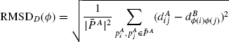
The mapping Ф defines a set of correspondences between the residues of the two proteins. The structures ![]() is called the length of the alignment. Given a structural alignment Ф between two structures PA and PB, and a transformation T of structure B onto A, a popular measure of the goodness of superposition is the root-mean-square deviation (RMSD), defined as
is called the length of the alignment. Given a structural alignment Ф between two structures PA and PB, and a transformation T of structure B onto A, a popular measure of the goodness of superposition is the root-mean-square deviation (RMSD), defined as

Given an alignment Ф, the optimal transformation >T, minimizing RMSD, can be computed in closed form using the method described in [31].
7.3.2 Algorithms for Structural Alignment and a Spectral Method
A typical attempt at designing a structural alignment algorithm involves defining an objective function that is a measure of goodness of a particular alignment, and optimizing the function over a permitted set of alignments. The RMSD is one such possible function. However, calculating RMSD requires calculating the optimal transformation T, which is computation intensive.
Objective functions based on pairwise distances (e.g., distance RMSD) [8], are popular because they don’t need computation of optimal transformations. Distance RMSD for an alignment Ф is defined as
where, ![]() is the distance between residues
is the distance between residues ![]() . The matrix d is also called the distance matrix of a protein structure. The RMSD is a distance function since the lower the RMSD, the better the alignment, and hence the closer the proteins in the (hypothetical) protein structure space. Section 7.4.2 proposes a kernel that captures a notion of similarity related to RMSDD.
. The matrix d is also called the distance matrix of a protein structure. The RMSD is a distance function since the lower the RMSD, the better the alignment, and hence the closer the proteins in the (hypothetical) protein structure space. Section 7.4.2 proposes a kernel that captures a notion of similarity related to RMSDD.
One problem in using distance RMSD as an objective function with protein structures, which are inherently noisy, is that it prefers alignments having lower lengths. This problem was addressed in the scoring function used by the popular protein structure comparison algorithm DALI [32]. Given an alignment Ф between two proteins PA and PB, the DALI score function is defined as
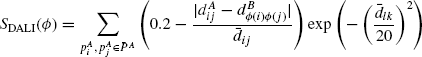
where ![]() . This function is relatively robust to differences in distances since any pair of residues for which the difference in distances is < 20% of the average distance contributes positively to the total score. Another feature of the scoring function is that it penalizes the average distance exponentially. Thus, contribution from relatively distant residues toward the overall score is negligible. This captures the idea that nearby atoms interact with much higher force than distant ones.
. This function is relatively robust to differences in distances since any pair of residues for which the difference in distances is < 20% of the average distance contributes positively to the total score. Another feature of the scoring function is that it penalizes the average distance exponentially. Thus, contribution from relatively distant residues toward the overall score is negligible. This captures the idea that nearby atoms interact with much higher force than distant ones.
The problem of matching pairwise distances can be posed as an inexact weighted graph matching problem [33]. In [20], we used this observation along with observation that interaction between nearby residues are more significant, to propose a new objective function for comparing two protein structures. This objective function is based on spectral projection vectors, and can be computed in O(n) time as compared to O(n2) time needed by the above objective function. Here, we recapitulate the definition briefly, and use it to motivate another kernel on protein structures in Section 7.4.
We start by defining the adjacency matrix A of a protein P as
Definition 7.3.2 Let A be the adjacency matrix of a protein P and ![]() be it eigenvalue distribution, such that the eigenvectors are arranged in decreasing order of the eigenvalues. The spectral projection vector f for P is defined as fi =
be it eigenvalue distribution, such that the eigenvectors are arranged in decreasing order of the eigenvalues. The spectral projection vector f for P is defined as fi = ![]() .
.
The spectral projection vector has the property of preserving neighborhoods optimally, while also preventing all projection values from being the same and thereby giving a trivial solution. Given spectral projection vectors fA and fB of two proteins PA and PB, respectively, and an alignment Ф between them, the spectral similarity score between the two proteins is defined as
where T is a parameter which makes the score function robust to small perturbations in f. The problem of optimizing Sspec with respect to all alignments, Ф, is solvable in polynomial time by posing it as an assignment problem [34]. Reference [20] proposes an efficient heuristic solution to this problem.
Section 7.4 proposes kernels on neighborhoods that capture the notion of similarity defined by the spectral similarity score. The structural alignment algorithm outlined above is very efficient, but does not work satisfactorily when the proteins being compared are of very different sizes. Section 7.3.3, outlines a method of tackling this problem using neighborhoods.
7.3.3 Problem of Indels and Solution Using Neighborhoods
In Section 7.3.2, we posed the problem of protein structure alignment as an inexact weighted graph matching problem, and derived a new similarity score based on spectral projection vectors. At the core of the method is the assumption that all residues in one protein have a matching residue in the second one. However, often proteins showing similar structure or function have many unmatched residues. These unmatched residues are called indels (insertions and deletions). Up to 60% indels are encountered in practical situations.
The way in which the algorithm in Section 7.3.2 was derived does not require the number of residues in the two structures to be the same. In fact, it works very well in practice when the number of indels is low. However, for a large number of indels (typically >40%) the method fails to perform as expected. This is due to the fact that the values of the spectral projection vector are changed by addition of extra residues.
Reference [11] proposes to address this problem by applying spectral algorithm to neighborhoods for calculating neighborhood alignments and growing the neighborhood alignments to get an alignment of entire structures. In [18] and this chapter, a similar paradigm is followed for designing kernels on protein structures. Here, following [11], we define two types of neighborhoods and give some biological justification behind each of them.
Definition 7.3.3 The ith structure neighborhood, ![]() of a protein P is a set of l residues closest to residue i in 3D space. So,
of a protein P is a set of l residues closest to residue i in 3D space. So,
The idea behind this definition is that there are highly conserved compact regions in 3D space, which are responsible for structure and functions of a given class of proteins. For example, structural motifs are the locally conserved portions of structure, while core folds are conserved regions responsible for the fold of the structure [35]. Similarly, active sites are conserved regions that are responsible for specfic functions. So, the neighborhoods falling in these conserved regions will have all the residues matched.
The algorithm (see Appendix A) considers all pairs of neighborhoods from both structures, and computes alignment between them. Based on these neighborhood alignments, transformations optimally superposing the aligned residues are computed. Alignment between the two protein structures is then calculated using a similarity measure derived from these transformations. The “best” alignment is reported as the optimal one.
Definition 7.3.4 The ith sequence neighborhood, ![]() of a protein P is the set of residues contained a sequence fragment of length l starting from residue i. So,
of a protein P is the set of residues contained a sequence fragment of length l starting from residue i. So,
Sequence neighborhoods were traditionally used by sequence alignment algorithms, e.g. Blast [36], and have been used in sequence-based kernels described in [5]. They have also been used in some structural alignment algorithms (e.g., CE) [21]. Sequence neighborhoods are sets of residues that are contiguous in the polymer chain, and hence are bonded together by covalent bonds. However, this may not be necessarily compact in 3D space. Also, note that unlike sequence processing algorithms, we include the 3D coordinates of residues along with residue type in the sequence neighborhood. In Section 7.4, we start by defining kernels on the two types of neighborhoods, which are them combined in various ways in Section 7.5 to define kernels on entire protein structures.
7.4 KERNELS ON NEIGHBORHOODS
Neighborhoods are subsets of residues of a protein structure that are compact in 3D space or in the protein sequence space. It is clear from the discussion in Section 7.3.3 that comparing neighborhoods for comparison of protein structures has some theoretical as well as experimental justification. We are interested in extending the same paradigm in design of kernels on protein structures. This section proposes various positive semidefinite kernels on neighborhoods. Section 7.4.1 defines kernels on protein structures using the kernels on neighborhoods defined here.
Each neighborhood Ni (either structure or sequence) is a set of l residues ![]() is the position of the residue in 3D space, and yj
is the position of the residue in 3D space, and yj ![]() Y is the amino acid type. It may be noted that while defining kernels we do not distinguish between the type of neighborhoods. However, some kernels make more sense with a specific type of neighborhood. We discuss this in more detail in Section 7.4.3.
Y is the amino acid type. It may be noted that while defining kernels we do not distinguish between the type of neighborhoods. However, some kernels make more sense with a specific type of neighborhood. We discuss this in more detail in Section 7.4.3.
We begin by defining various kernels capturing similarity between the types of amino acids in the two neighborhoods, then define kernels capturing similarity between 3D structures of the two neighborhoods, and finally describe two methods to combine these two kernels to get kernels on neighborhoods.
7.4.1 Sequence-Based Kernels on Neighborhoods
Amino acid types are one of the most commonly used features in comparison of proteins. There are 20 different types of amino acids are found in proteins. First, we define kernels capturing the similarity between different types of amino acids. The simplest similarity measure is to assign unit similarity between identical amino acids and zero similarity to the rest. This gives us the identity kernel KI on Y × Y:
Another popular measure of similarity between amino acid types is given by the substitution matrices (e.g., the BLOSUM62 matrix) [37]. BLOSUM matrices give the log of likelihood ratio of actual and expected likelihoods. Unfortunately, the BLOSUM62 matrix is not positive semidefinite. We use the diffusion kernel [27] technique to construct a positive semidefinite kernel Kblosum on Y × Y, from the blosum matrix:
where Sblosum is the blosum substitution matrix.
Representative Residue Kernel. The amino acid kernels can be combined in various ways to give kernels on neighborhoods. One simple way is to summarize the entire neighborhood by a single representative residue. The choice of representative residue is very natural in the case of a structure neighborhood, since it has a central residue. In case of sequence neighborhoods, the representative residue is taken as the starting residue of the sequence fragment.
Let ![]() be some positive semidefinite kernel on amino acids. The representative residue kernel Krep on neighborhoods is defined as
be some positive semidefinite kernel on amino acids. The representative residue kernel Krep on neighborhoods is defined as
where, yrep(Ni) is the amino acid type of representative residue of neighborhood Ni chosen as described above.
All Pair Sum and Direct Alignment Kernels. The above kernel is derived by summarizing neighborhoods with their representative residues. Neighborhoods can also be viewed as sets of residues, thus allowing us to use existing set kernels. Many kernels have been proposed on sets (e.g., [2,3,5]). Here, we propose two kernels motivated from set kernels.
Let A and B be two d × c matrices. It was shown in [25], that if k is a PSD kernel on ![]() is a PSD kernel, Ai being the ith column of A. This can be generalized to arbitrary objects (amino acids in this case) rather than vectors in Rc:
is a PSD kernel, Ai being the ith column of A. This can be generalized to arbitrary objects (amino acids in this case) rather than vectors in Rc:
Definition 7.4.1 Let ![]() be a neighborhood, and
be a neighborhood, and ![]() be any amino acid kernel. The direct alignment kernel Kdiral between neighborhoods Ni and Nj is defined as
be any amino acid kernel. The direct alignment kernel Kdiral between neighborhoods Ni and Nj is defined as
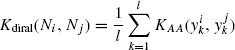
The fact that Kdiral is positive semidefinite follows trivially from the above discussion and the fact that l is a positive constant. This kernel assumes a fixed serial ordering of the residues. This is applicable in the case of sequence neighborhoods.
Another case is where such an ordering is not known. For such a case, [4] defines general kernels on matrices that have the same number of rows, but a different number of columns. Let A and B be n × k and n × q matrices respectively. Let G and F be n× n and q × k matrices, such that G and extension of F to m × m matrices, m = max(n,q,k), is a positive semidefinite matrix. Then, ![]() is a PSD kernel. Simplifying this, it can be shown that
is a PSD kernel. Simplifying this, it can be shown that ![]() is a PSD kernel. Generalizing this result, we can define sequence-based kernels on neighborhoods.
is a PSD kernel. Generalizing this result, we can define sequence-based kernels on neighborhoods.
Definition 7.4.2 Let ![]() be a neighborhood, and KAA :
be a neighborhood, and KAA : ![]() be any amino acid kernel. The all pair sum kernel, Kallpair, between neighborhoods Ni and Nj is defined as
be any amino acid kernel. The all pair sum kernel, Kallpair, between neighborhoods Ni and Nj is defined as
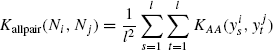
The fact that Kallpair is PSD follows trivially from the above discussion. This kernel is useful in case of structure neighborhoods where there is no ordering between residues. In Section 7.5., we use a similar technique to define kernels on protein structures.
Permutation Sum Kernel. The set kernel derived above adds up similarity between all pairs of residues in the two neighborhoods. Another interesting kernel is where all possible assignments of one residue to other is considered. In case of neighborhoods of fixed size, this implies considering all permutations of the residues in one of the neighborhoods. We use the idea of convolution kernels [19] to arrive at this notion.
Let x ![]() X be a composite object formed using parts from
X be a composite object formed using parts from ![]() be a relation over
be a relation over ![]() such that
such that ![]() is composed of
is composed of ![]() be kernels on X1,…,X_m, respectively. The convolution kernel K over X is defined as
be kernels on X1,…,X_m, respectively. The convolution kernel K over X is defined as
It was shown in [19], if K1,…,Km are symmetric and positive semidefinite, so is K.
In our case, the composite objects are the neighborhoods Ni’s and the “parts” are the residues ![]() in those neighborhoods. The relation R is defined as R(p1, …, plNi) is true iff Ni = p1,…,pl. Thus, the set R-1(Ni) becomes all permutations of
in those neighborhoods. The relation R is defined as R(p1, …, plNi) is true iff Ni = p1,…,pl. Thus, the set R-1(Ni) becomes all permutations of ![]() . In other words,
. In other words, ![]() being the set of all permutations of l numbers.
being the set of all permutations of l numbers.
Definition 7.4.3 Let ![]() be a neighborhood, and
be a neighborhood, and ![]() be any amino acid kernel. The permutation sum kernel Kperm between neighborhoods Ni and Nj is defined as
be any amino acid kernel. The permutation sum kernel Kperm between neighborhoods Ni and Nj is defined as
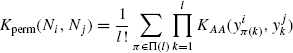
To see that Kperm is a PSD kernel, notice that permuting residues in both neighborhoods will result in all possible assignments being generated l! times. The convolution kernel following the above discussion is
Since the above kernel is PSD (using theorem 1 in [19]), dividing it by (l!)2, we get Kperm, which is also PSD. In Section 7.4.2, we use the same idea to define various structure based kernels on neighborhoods.
7.4.2 Structure-Based Kernels on Neighborhoods
Each residue pi of a protein structure P can be represented as two parts: the position x}i and the residue type (attribute) yi. In Section 7.4.1, we defined many kernels on neighborhoods using kernels on residue type yi for each residue. Kernels on the residue type are easier to define since the residue types are directly comparable. On the other hand, positions of residues from different protein structures are not directly comparable as they may be related by an unknown rigid transformation.
This section defines kernels on neighborhoods using the structure of the neighborhood described by the position of residues. We begin, by using the spectral projection vector derived in Section 7.3.2 (Definition 7.3.2). Note that the spectral projection vector can be thought of as assignment of one real number to each residue in the neighborhood, when used for matching neighborhoods (Section 7.3.3). Also, it can be inferred from Eq. 7.6), that the components of the spectral projection vector can be compared directly.
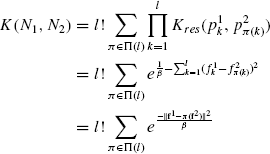
Spectral Neighborhood Kernel. Let ![]() be two neighborhoods, each having l residues. Let f1 and f2 be the spectral projection vectors (Definition 7.3.2 for these neighborhoods. The residue kernel, Kres, between ith residue of N1, p1i, and jth residue of N2, p2j, is defined as the decreasing function of the difference in spectral projection:
be two neighborhoods, each having l residues. Let f1 and f2 be the spectral projection vectors (Definition 7.3.2 for these neighborhoods. The residue kernel, Kres, between ith residue of N1, p1i, and jth residue of N2, p2j, is defined as the decreasing function of the difference in spectral projection:
β being a parameter. This kernel is PSD since it is essentially a Gaussian kernel. Note that the spectral projection vector trick was used to find a quantity that is comparable between residues of two structures.
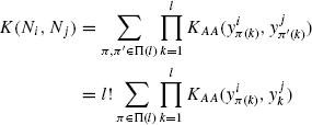
Now, we can use the techniques used in Section 7.4.1 to define kernels on neighborhoods. We use the convolution kernel method since it also gives a relation to the spectral similarity score [Eq. 7.6)]. In our case, X is the set of all neighborhoods and X1, …, Xm are all sets of all the residues pi’s from all the neighborhoods. Here, note that even if the same residue appears in different neighborhoods, the appearances will be considered to be different, since their spectral projection values are different.
Following the discussion in Section 7.4.1, the relation R is defined as R(p1,…,pl,N) is true iff N = p1, …,pl. Since, all the Xi’s have all the residues from N, the cases for which R can hold true are the permutations of residues of N. Since this can happen for both N1 and N2, each combination of correspondences occurs l! times. Thus, using Ki = Kres, i = 1, …, l in Eq. 7.10, the kernel becomes
where, fi is the spectral projection vector of Ni and Π(l) is the set of all possible permutations of l numbers.
Definition 7.4.4 Let ![]() be a neighborhood, and fi be the spectral projection vector corresponding (Definition
ef{def:specvec}) to Ni. The spectral kernel, Kspec, between neighborhoods Ni and Nj is defined as
be a neighborhood, and fi be the spectral projection vector corresponding (Definition
ef{def:specvec}) to Ni. The spectral kernel, Kspec, between neighborhoods Ni and Nj is defined as
Positive semidefiniteness of this kernel follows trivially from the above discussion. Note that, computation of this kernel takes exponential time in l. However, since l is a parameter of choice, and is usually chosen to be a small value (six in our experiments), the computation time is not prohibitive. Next, we show a relation between Kspec and Sspec [Eq. 7.6)].
Theorem 7.4.1 Let Ni and Nj be two neighborhoods with spectral projection vectors fi and fj. Let Sspec(Ni,Nj) be the score of alignment of Ni and Nj, obtained by solving problem in Eq. 7.6), for a large enough value of T such that all residues are matched.
Proof: Let π* be the permutation that gives the optimal score Sspec(Ni,Nj). By definition, ![]() .
.
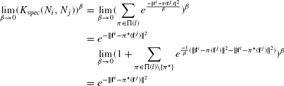
The last step is true since ![]() is always positive, and hence
is always positive, and hence ![]() is 0. Combining the above equations, we get the result.
is 0. Combining the above equations, we get the result.
Pairwise Distance Substructure Kernel. The previous kernel used the spectral projection based formulation to measure the similarity between neighborhoods. However, since the size of neighborhoods are usually small, we can also capture the similarity between pairwise distances of the two neighborhoods [Eq. 7.3)]. We do this by using the convolution kernel techniques [19].
In this case, X is the set of all neighborhoods and X1,…,Xm are sets of all pairwise distances dij, i < j between the residues from all neighborhoods. For each neighborhood of size l, we consider all pairwise distances between residues of that neighborhood. So, m = l(l-1)/2. We define the pairwise distance vector, f of a neighborhood ![]() as:
as:
The relation R is defined as R(d,N) is true iff f is a pariwise distance vector of N.
Definition 7.4.5 Let ![]() be a neighborhood, and di be the pairwise distance vector of
be a neighborhood, and di be the pairwise distance vector of ![]() . The pairwise distances kernel, Kpd, between neighborhoods Ni and Nj is defined as
. The pairwise distances kernel, Kpd, between neighborhoods Ni and Nj is defined as
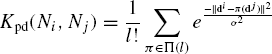
where, by notation ![]() .
.
Under the condition that all residues from two neighborhoods Ni and Nj have a matching residue in the other neighborhood, a decreasing function of optimal distance RMSD [Eq. 7.3)] can be used as a similarity measure between the two neighborhoods. Since all residues are matching, the space of all mapping become all permutations of the residues of one neighborhood while keeping the other fixed. By using the above definition of a pairwise distance vector, we define the similarity score as
Next, we show a relation similar to that in Theorem 1, between Kpd and Sdrmsd.
Theorem 7.4.2 Let Ni and Nj be two neighborhoods with pairwise distance vectors di and dj. Let Sdrmsd(Ni,Nj) be the similarity score between Ni and Nj, obtained by solving problem in Eq. 7.13).
Proof is essentially similar to that of Theorem 1.. Both Theorems 1 and 2 show that for low values of β and σ the structure kernels are related to the alignment scores between neighborhoods. This is also demonstrated in the experiments in Section 7.6.4. Next, we describe two methods for combining kernels based on sequence and structure, to get general kernels on neighborhoods.
7.4.3 Combined Sequence and Structure-Based Kernels on Neighborhoods
According to our definition, each residue in a protein structure has two components: position in 3D space that describes the structure, and a type (or attribute) that describes the sequence. This can be viewed as an attributed pointset ([10]), which is a set of points in an Euclidean space with an attribute attached to each point. The main difference between position and attribute is that attributes are comparable directly, while positions can be related by a rigid transformation, and hence are not comparable directly.
In [10], we proposed kernels on attributed pointsets and used them for various tasks in computer vision. Kernels capturing position and attribute similarity were combined by weighting the position kernel with the attribute kernel. Here, we begin by weighting the structure based kernels with the sequence-based kernels.
Definition 7.4.6 Let Ni and Nj be two neighborhoods. Let Kseq and Kstr be sequence- and structure-based kernels on neighborhoods. The weighting kernel, Kwt, on neighborhoods is defined as
where Kwt is PSD, since it is a pointwise product of two PSD kernels. In this chapter, the choices explored for Kseq are Krep, Kallpair, Kdiral, and Kperm, while those for Kstr are Kspec and Kpd.
Another popular method of combining information from multiple kernels, mainly popularized by multiple kernel learning literature ([38,39]), is to use a linear combination of the kernels. Following this paradigm, we define our next kernel as a convex combination of sequence- and structure-based kernels.
Definition 7.4.7 Let Ni and Nj be two neighborhoods. Let Kseq and Kstr be sequence- and structure-based kernels on neighborhoods. The convex combination kernel Kcc on neighborhoods is defined as
where, γ ![]() [0,1] is a parameter. This kernel is PSD since it is a linear combination of PSD kernels with positive coefficients. The same choices for Kseq and Kstr as above are explored. In Section 7.5, we combine the neighborhood kernels, Kwt and Kcc, to get kernels on entire protein structures.
[0,1] is a parameter. This kernel is PSD since it is a linear combination of PSD kernels with positive coefficients. The same choices for Kseq and Kstr as above are explored. In Section 7.5, we combine the neighborhood kernels, Kwt and Kcc, to get kernels on entire protein structures.
7.5 KERNELS ON PROTEIN STRUCTURES
Section 7.4 defined various kernels on neighborhoods. This section describes two ways of combining these kernels to get kernels on entire protein structures. The first method uses set kernels by viewing each protein as a set of neighborhoods. We show that these kernels are related to the well-known spectrum kernels [5]. The second method uses known alignments to increase the accuracy of similarity measure.
7.5.1 Neighborhood Pair Sum Kernels
One way of combining neighborhood kernels for deriving kernels on protein structures is by viewing proteins as a set of neighborhoods. Various strategies could be used to choose the neighborhoods that describe a protein structure. For example, we could choose a minimal set of neighborhoods that cover all the residues in a protein. However, this may not have a unique solution, which may lead to a comparison of different neighborhoods of similar structures, and hence low similarity between similar structures.
For structure neighborhoods, we consider neighborhoods centered at each residue. This ensures that all residues are part of at least one neighborhood. For sequence neighborhoods, we consider neighborhoods starting at each residue except the last l-1 in the protein sequence since there can not be any neighborhoods of length l starting at them.
We view a protein structure as a set of constituent neighborhoods. Thus, a protein PA, described by nA neighborhoods, is represented as ![]() . From the set kernels described in Section 7.4.1, only the representative element kernels and all pair kernels are applicable since the number of neighborhoods in two proteins PA and PB may not be the same. Considering only one neighborhood, is generally not a good representation of the entire protein structure. Thus we use the all pair sum kernel for defining kernels on protein structures.
. From the set kernels described in Section 7.4.1, only the representative element kernels and all pair kernels are applicable since the number of neighborhoods in two proteins PA and PB may not be the same. Considering only one neighborhood, is generally not a good representation of the entire protein structure. Thus we use the all pair sum kernel for defining kernels on protein structures.
Definition 7.5.1 Let PA and PB be two proteins represented in terms of constituent neighborhoods as ![]() be a kernel on neighborhoods. The neighborhood pair sum kernel, Knps between the two proteins is defined as
be a kernel on neighborhoods. The neighborhood pair sum kernel, Knps between the two proteins is defined as
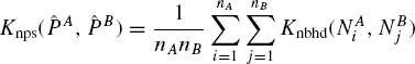
where Knps is a PSD kernel because it is of the form ψA ψB K(A,B) where K(A,B) is a PSD kernel and ψA is a function of only A. The parameter Knps can be computed in O(nA nB) time. Next, we show a relation between between Knps and the spectrum kernel [5].
The spectrum kernels were designed for protein sequence classification using support vector machines. For every protein sequence s, [5] defines the k-spectrum-based feature map Θk(x) indexed by all k length subsequences ![]() , where θa(s) is the number of occurrences of a in s. The k-spectrum kernel is defined as:
, where θa(s) is the number of occurrences of a in s. The k-spectrum kernel is defined as: ![]() .
.
Theorem 7.5.3 Let P and P′ be two proteins with representations ![]() be their sequences. Then, there is a sequence kernel on neighborhoods, Kseq, for which
be their sequences. Then, there is a sequence kernel on neighborhoods, Kseq, for which ![]() , where Knbhd = Kcc with γ = 1, and sequence neighborhoods of length l are used to represent P and P′.
, where Knbhd = Kcc with γ = 1, and sequence neighborhoods of length l are used to represent P and P′.
Proof: Kspectruml(s,s′) computes the number of common subsequences of length l between s and s′, where each occurrence of a subsequence a is considered different. This is because ![]() , thus adding up products of counts every subsequence.
, thus adding up products of counts every subsequence.
Observe that all nonzero entries in Θl(s) precisely correspond to sequence neighborhoods of size l in ![]() . Consider the kernel on neighborhoods
. Consider the kernel on neighborhoods ![]() are identical, 0 otherwise. The parameter Knbhd = Kseq since γ = 1. So,
are identical, 0 otherwise. The parameter Knbhd = Kseq since γ = 1. So,
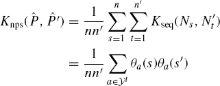
This result shows that when restricted to use only sequence related information, Knps is essentially the length normalized version of Kspectrum. Note that a similar result can be derived for the mismatch kernels [5] with an appropriate choice of Kseq. Unfortunately, the feature map representation used to derive spectrum kernels cannot be extended directly to define kernels on structures since the feature space will be infinite. Section 7.5.2 defines kernels that use alignments generated by external structural alignment programs.
7.5.2 Alignment Kernels
Section 7.5.1 defineds kernels on protein structures that do not need any extra information. The kernels add up similarity between all pairs of neighborhoods in the two protein structures. However, any neighborhood in a protein structure is expected to be similar to only one neighborhood in the other structure. So, adding the kernels values for other pairs of neighborhoods introduces noise in the kernel value that reduces the classification accuracy.
This section alleviates this problem by utilizing alignment between residues given by a structural alignment program to compute kernels. The correspondences between residues given by a structural alignment induces correspondence between the structure neighborhoods centered at these residues. The naive structural alignment kernel adds up kernels between the corresponding neighborhoods.
Definition 7.5.2 Let Pi and Pj be two proteins represented in terms of constituent structure neighborhoods as ![]() be a kernel on neighborhoods. Let Фij be an alignment between Pi and Pj. The naive alignment kernel, Knal between the two proteins is defined as
be a kernel on neighborhoods. Let Фij be an alignment between Pi and Pj. The naive alignment kernel, Knal between the two proteins is defined as
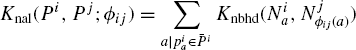
Note that here only structure neighborhoods can be used since some residues will not have a corresponding sequence neighborhood. Unfortunately, this kernel is not necessarily positive semidefinite. Though SVM training algorithm has no theoretical guarantees for a kernel matrix that is not PSD, they work well in practice.
While many methods have been suggested for learning with non-PSD kernels [40], most of them require computation of singular values of the kernel matrix. This may be computationally inefficient or even infeasible in many cases. Moreover, in most cases, the values of the kernel function do not remain the same as the original kernel function. Another kernel is proposed based on the alignment kernel, which while keeping the off-diagonal terms intact and only modifying the diagonal terms, is always positive semidefinite.
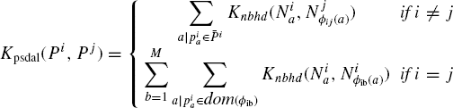
Definition 7.5.3 Let D = P1,…,PM be a dataset of M proteins represented in terms of constituent structure neighborhoods as ![]() and Knbhd be a kernel on neighborhoods. Let Фij be an alignment between
and Knbhd be a kernel on neighborhoods. Let Фij be an alignment between ![]() . The PSD alignment kernel, Kpsdal between the two proteins Pi and Pj is defined as
. The PSD alignment kernel, Kpsdal between the two proteins Pi and Pj is defined as
where dom(Фib) is the domain of function Фib, which is the set of all residues participating in the alignment Фib from structure Pi. Notice that Kpsdal can be computed in an incremental way, which is not trivial for methods that require singular value decomposition. Next, we show that Kpsdal is indeed PSD.
Theorem 7.5.4 The parameter Kpsdal is positive semidefinite if Knbhd is positive valued.
Proof: Let Lmax be the maximum length of alignments between all pairs of proteins in the dataset D. Consider the ![]() having one row for each protein in the dataset. Each row has
having one row for each protein in the dataset. Each row has ![]() blocks of length Lmax corresponding to each pairwise alignment (including alignment of every structure with itself). For rows corresponding to proteins i and j, the
blocks of length Lmax corresponding to each pairwise alignment (including alignment of every structure with itself). For rows corresponding to proteins i and j, the ![]() element of the block for alignment Фij is equal to
element of the block for alignment Фij is equal to ![]() . The index k runs over all the correspondences in the alignment. For alignments that have length smaller than Lmax, put the remaining entries to be zero. It can be seen that Kpsdal = H HT Since, each entry in Kpsdal is a dot product between two vectors, Kpsdal is positive semidefinite.
. The index k runs over all the correspondences in the alignment. For alignments that have length smaller than Lmax, put the remaining entries to be zero. It can be seen that Kpsdal = H HT Since, each entry in Kpsdal is a dot product between two vectors, Kpsdal is positive semidefinite.
This theorem can also be proved using the result that diagonally dominant matrices (matrices having the property Aii ≥ ∑j=1n |Aij|) are PSD. Note that, Knbhd needs to be positive valued and not positive semidefinite. So, this method can get a kernel from any postive valued similarity measure on the neighborhoods. Unfortunately, diagonal dominance of a kernel often reduces its classification accuracy (e.g., see [41, 42]).
Computational Complexity. Time complexity of the neighborhood kernels is O(1), since size of the neighborhoods is a user-defined parameter, rather than a charateristic of data. For neighborhood size l, the time complexities of Krep, Kdiral,Kallpair,Kperm,Kspec, and Kpd are O(1), O(l), O(l2), O(l!), O(l!) and O(l!), respectively. Since for most experiments, l was fixed at a very low value of 6, the exponential complexity of Kperm,Kspec, and Kpd does not pose a major problem to computational feasibility.
The time complexity of Knps is O(n1n2), where n1 and n2 are the number of neighborhoods in the two proteins being compared. Time complexity of Knal is O(min(n1,n 2). The parameter Kpsdal can be implemented in amortized time complexity of O(n), n being the maximum length of alignment. Memory requirements of all the kernels are O(n1+n2), which is necessary for storing the proteins in memory. In Section 7.6, we report results of experiments conducted for validating the kernels developed here on the task of protein structure classification.
7.6 EXPERIMENTAL RESULTS
Extensive experimentation was conducted in order to both demonstrate the practical applicability of the kernels proposed above on real protein structures, and to study properties of the proposed kernels. Section 7.6.1 describes the data set, the experimental procedure, and the quantities observed. Section 7.6.2 reports representative and average results for various types of kernels and compares them with classification performed using a popular protein structure comparison method CE [21]. Section 7.6.5 studies the effects of various parameters on the classification performance of the kernels. Section 7.6.5 describes results of experiments with spectrum kernels in order to demonstrate the difficulty of the current task.
7.6.1 Experimental Setup
The kernels proposed above were tested extensively on the well-known structural classification database called SCOP [12]. The experiments were designed so as to test utility of the proposed kernels toward the practical and difficult problem of classifying structures having very low sequence identity (< 40%). The results were compared with a state of the art protein structure alignment algorithm, CE [21], which was found to be the top performer in [43].
The kernels developed were implemented in C using GCC/GNU Linux. OpenMPI over LAM was used on a cluster to speed up the computations. Eigenvalue computations were done using Lapack [44], and SVM classifications were done using Libsvm [45]. The protein structures were obtained from ASTRAL [46].
Data Set Construction. The task chosen was to classify a data set of proteins having < 40% sequence identity between any pair of proteins. This task is both difficult and relevant to computational biologists, since most standard sequence processing algorithms (e.g., BLAST [36]), cannot identify many relationships between proteins having low sequence similarity [47]. Thus, kernels utilizing the structure information to achieve accurate results on such difficult problems are highly useful. Also, the ASTRAL compendium [46] provides a 40% nonredundant data set, which is the lowest redundancy cutoff provided by ASTRAL.
We chose the classification at the superfamily level of SCOP. This level captures functional and distant evolutionary relationships, where 21 superfamilies were detected that had at least 10 proteins at 40% sequence non-redundance (in SCOP 1.69). The structural classification is performed using 21 one versus all classification problems. In order to get a balanced problem, a randomly chosen set of 10 proteins from other classes is used as the negative dataset for each class. In order to get a stable estimate of the classification accuracy, this experiment is repeated 100 times and the average is reported.
Similar tasks have been attempted by [17] and [16]. However, we concentrate on structural classification rather than functional annotation, since we are more interested in studying the properties of the proposed kernels than exploring possible diverse applications. Also, the task we have chosen is more difficult since we attempt to classify the 40% nonredundant data set, as compared to say the 90% nonredundant data set used in [16]. This allows us to concentrate on a much smaller data set (9,479 domains instead of 97,178 in SCOP 1.73), and thus allows us to use more computationally intensive algorithms.
Experimental Procedure. We use the leave-one-out cross-validation as the basic test for the classifier, due to a small number of datapoints per class. Leave-one-out cross-validation was also used in [17]. The predicted labels are used to calculate accuracies on positive and negative classes and receiver operating characterstic (ROC) curves [48]. For a group of kernels, the average results are reported in the form of area under ROC curve (AUC) [48] and average classification accuracies; and the variance around average as maximum and minimum classification accuracies. The area under ROC curve (AUC) [48] is used as the primary index for judging the quality of a classifier and AUC is also used in [16].
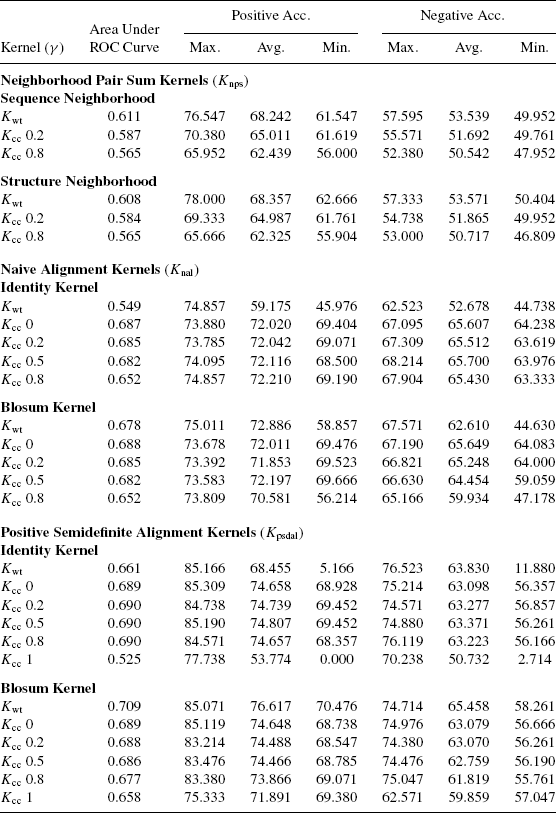
Each combination of the type of amino acid kernels, sequence- and structure-based kernels on neighborhoods, and method of combination of sequence and structure based kernels is called a type of kernel. Table 7.1 gives the types of kernels for which experiments were performed. Due to intuition from biology, all pair sum kernels were computed only for structure neighborhoods and direct alignment kernels were computed only for sequence neighborhoods. A total of 44 types of kernels were experimentally evaluated for various parameter values. Average results for each type of sequence and structure kernel are in Section 7.6.3. Due to lack of space, detailed results for each type of kernel is provided in the supplementary material.
TABLE 7.1 Types of Kernels for Which Experiments Were Performed
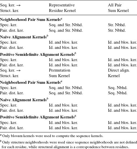
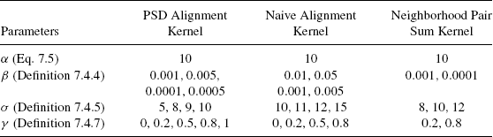
Table 7.2 shows the values of parameters for which experimental results are reported. These parameters were found by trial and error to be appropriate for current task. Section 7.6.4 compares the performance of various kernels for these parameter values. Detailed results are reported in the supplementary material.
TABLE 7.2 Values of Various Parameters for Which Experimental Results are Reported
7.6.2 Validation of Proposed Kernels
This section validates the effectiveness of the proposed kernels on the above mentioned task. All the kernels mentioned above were used to train classifiers for the task. We report representative and average results with variances for the kernels. These results are compared with the state of the art protein structure comparison tool called CE [21]. Detailed results are available in the supplementary material.
Table 7.3 reports representative results for various kernels studied here and compares them with the results obtained from CE [21]. All the positive semidefinite alignment kernels, except the ones that use sequence information only (for γ = 1), perform comparably or better than CE. Thus, kernel based methods can be used along with SVMs to achieve performance comparable to state-of-the-art methods in computational biology.
TABLE 7.3 Representative Results for Knps (def. 7.5.1), Knal (def. 7.5.2), Kpsdal (def. 7.5.3), and CE [21]
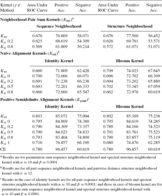
The other kernels do not perform as well as positive semidefinite alignment kernels. For neighborhood pair sum kernels, this is due to inaccuracy in computing the similarity values arising out of the fact that they sum up similarities between all pairs of neighborhoods. For the naive alignment kernels, this is due to the fact that they are not necessarily positive semidefinite. Also, the naive alignment kernels perform slightly better than the neighborhood pair sum kernels, since they use the extra information provided by the structural alignment and only add up similarities between equivalent neighborhoods.
We also observe that for neighborhood pair sum (NPS) kernels, the weighting kernels perform slightly better than the linear combination kernels. However, for the alignment kernels, the performance of weighting kernels, as well as the linear combination kernels are similar. The reason is that for NPS kernels, multiplication of structure similarity component by sequence similarity leads to more effective weighing down of similarity values for the noncorresponding neighborhoods, thereby increasing the influence of similarity between corresponding neighborhoods. This principle was also used in [10] to improve the performance kernels for face recognition. This problem is not present in alignment kernels, and hence there is not much difference in accuracies of weighting and linear combination kernels.
Note that for linear combination NPS kernels there is a gradual decrease in their performance with the increase in value γ. Hence, there is an increase in component sequence similarity. This difference is not observed in the case of alignment kernels. However, there is a sharp decline in performance of alignment kernels when the component of structural similarity becomes zero (for γ = 1). From these observations, we can conclude that the structural similarity component is much more useful than sequence similarity component for the present task. This is also consistent with the biological intuition that for distantly related proteins, structural similarity is higher than sequence similarity.
Another observation is that positive classification accuracy is much higher than negative classification for all kernels. The reason is that a multi-class classification problem was posed as many binary class classification problems and the average accuracy over all problems is reported. Thus for each classification problem, the positive class is a true class while the negative class is an assortment of all other classes. This explains the asymmetry in the classification accuracies.
Figure 7.1 presents the ROC curves for the representative kernels reported above, and compares them with those from CE [21]. The NPS kernels (Figs. 7.1a and b) perform worse than CE. However, some of the naive alignment kernels (Figs. 7.1c and d) perform comparatively with CE till 30% of the false positives. After which their performance declines. Interestingly, the positive semidefinite alignment kernels perform much better than CE for low false positive rates. For example, the positive semidefinite weighting kernel gives ∼85% true positives at 25% false positives, while CE gives only about 60% true positives at the same false positive level. However, CE performs better than the kernel based classifiers at false positive rates >35%. Overall, some kernels perform marginally better than CE (according to AUC reported in Table 7.3).
FIGURE 7.1 Representative results for Knps (def. 7.5.1), Knal (def. 7.5.2), Kpsdal (def. 7.5.3), and CE [21] Parts (a) and (b) show ROC curves for Knps with sequence and structure neighborhoods, respectively. Parts (b) and (d) show ROC curves for Kmax with identity and blosum amino acid kernels. Parts (e) and (f) show ROC curves for Kprdal with identity and blosum amino acid kernels.
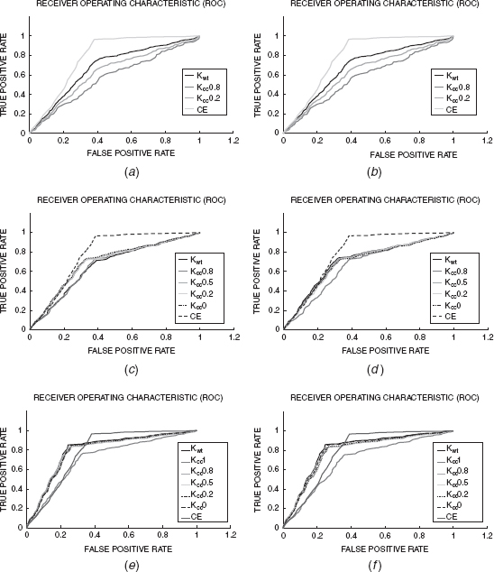
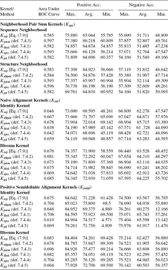
Table 7.4 reports the average results for different kernels over all types of kernels and parameter values listed in Tables 7.1 and 7.2. All the observations made with the representative results are also observed for the average results.
Variance in the performance is reported using maximum and minimum classification accuracy of the classifiers. Some classifiers obtained using Kwt and Kcc(γ = 1) show very low minimum classification accuracy. This is due to numerical problems that arise due to the sequence-based kernel taking very low values.
It was observed that the variance in performance of the weighting kernels is much higher than the comvex combination kernels. Thus, weighting kernels are much more sensitive to variation in parameters than the convex combination kernels. This can be attributed to a more profound effect of the multiplication operation.
TABLE 7.4 Average Results for Knps (def. 7.5.1), Knal (def. 7.5.2), and Kpsdal (def. 7.5.3)
From the above observations, we conclude that overall the kernels proposed in this chapter provide a comprehensive and effective scheme for designing classifiers for proteins having low sequence similarity. The weighting method generates more accurate albeit sensitive classifiers than convex combination. Also, in the case of convex combination kernels, kernels capturing structure information turn out to be more effective for the current purpose than kernels capturing sequence similarity.
7.6.3 Comparison of Different Types of Neighborhood Kernels
This section studies the relative performance of different types of neighborhood kernels developed in this chapter. Table 7.5 reports the average results for all types of kernels, averaged over all parameter values and other types of kernels. More detailed results are reported in the supplementary material.
TABLE 7.5 Average Results for Different Types of Neighborhood Kernels
We observe that average performance of various types of sequence neighborhood kernels is similar for a given type of kernel on the whole protein. This can be attributed to the fact that sequence information is not very useful for the present task. Thus, different types sequence neighborhood kernels are restricted by the nature of information provided to them.
The spectral structure neighborhood kernel is performing marginally better than the pairwise distance structure neighborhood kernel. Except the naive alignment kernel, the maximum accuracies achieved by spectral neighborhood kernel-based classifiers is significantly higher than those achieved by pairwise distance neighborhood kernel-based classifiers. For naive alignment kernels, their performances are comparable. The reason that protein structures data is noisy by nature. The spectral projections are more robust to noise than pairwise distances.
The variance in accuracy was also not found to be related to the type of neighborhood kernel. Thus, we conclude that spectral kernels are slightly better than pairwise distance kernels for the current task. A characterization of the sequence neighborhood-based kernels for various kinds of tasks remains an open question.
7.6.4 Effects of Parameter Values
This section studies the effect of various parameter values on the classification accuracy of the resulting kernels. There are two parameters in for the spectral kernel Kspec(def. 7.4.4), α [Eq. 7.5)] and β (def. 7.4.4). The value of α is fixed at 10, which is determined to be the optimal value in previous experiments [11]. β was allowed to vary in the set indicated in Table 7.4. Table 7.7 reports average results on the different types of kernels and various values of β. The pairwise distance kernel Kpd (def. 7.4.5) has one parameter, σ (def. 7.4.5). The parameter σ was allowed to take values in the set provided in Table 7.2. Table 7.7 reports average results for various vales of σ. Detailed results are provided in the supplementary material.
For convex combination kernels, the parameter γ (def. 7.4.7) is varied to study the effect of sequence- and structure-based kernels on classification accuracy. This study was reported in Section 7.6.2 along with the average results. Results are presented in Table 7.4. Hence, we do not repeat it here.
TABLE 7.6 Average Results for the Parameter β

From Table 7.6, we observe that in most cases, the classifier accuracy increases with decrease in value of β. This finding is in accordance with the result in Theorem 1, which says that as β → 0, the value of Kspec approaches an increasing function of the spectral alignment score, which was motivated to be a good measure of structural similarity in Section 7.3.2. The decrease in average performance with a decrease in β, in the case of naive alignment kernels, is due numerical errors in some of the kernels, which is evident from the < 50% minimum classification accuracy (which is achieved by a random classifier).
We also observe that the variance in classification accuracy increases with decrease in the value of β. This results because we make the kernel more sensitive to difference in spectral projection values by the decreasing value of β. Thus, even for small noise in the spectral projections, the kernel value turns out to be zero and does not contribute toward making better classifications. Thus, even though some classifiers are very good, a lot of them are highly sensitive to the noise in data. This results in a wide variance in the classifier performance.
TABLE 7.7 Average Results for the Parameter σ

Table 7.7 reveals similar trends with σ as shown in Table 7.6 with β. As suggested by Theorem 2, an increase in the value of σ results in a decrease in classification performance. For naive alignment kernels, the performance does not vary much.
However, the increase in variance is not apparent for the current set of parameters. This is due to the fact that the range of parameters chosen for experimentation was not sufficiently extreme to induce numerical instability in most kernels. This is also supported by the fact that minimum classification accuracy is fairly high in most kernels.
From these observations, we conclude that in accordance with theorems described in Section 7.4.2, decreasing values of β and σ increases the classifier performance, but also makes the classifier more sensitive to noise in data.
7.6.5 Comparison with the Spectrum Kernel
Section 7.5.1 shows that the spectrum kernels [5] turn out to be a special case of our kernels, when restricted to using sequence information alone. We implemented mismatch kernels [5.49] of which spectrum kernels are a special case and performed similar experiments on our dataset as we did for validating the kernels developed here. This was done to ascertain the difficulty of the our task, and to demonstrate that structure information is highly useful in the context such a task. This section reports results from these experiments.
The spectrum kernels are a special case of mismatch kernels for which the number of allowed mismatches is 0. We experimented with the window sizes of 4 and 5, and allowed mismatch of 0 and 1. The original authors reported that spectrum kernels performed best for window size 4[49], which was reconfirmed in our experiments.
Table 7.8 reports the results from experiments conducted with spectrum kernels, the best result obtained used a positive semidefinite alignment kernel using sequence information only (Kpsdal(seq)), overall best result obtained using positive semidefinite alignment kernel (Kpsdal(best)), and CE [21]. It is clear that even the best performing spectrum kernel performs quite poorly on the current task, thereby demonstrating the difficulty of the current task and emphasizing the need to use structure information. It can also be observed that using alignment information along with only sequence based kernels (Kpsdal(seq)), considerably improves the classification accuracy. Also, using the structure information in neighborhood pair sum kernels, of which spectrum kernels are a special case, improves the classification performance (AUC: 0.676 Table 7.3). Finally, both CE and Kpsdal(best) achieves reasonable accuracies on the same task.
TABLE 7.8 Results for Classification With Spectrum Kernels and Other Methods Compared Above
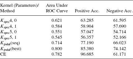
FIGURE 7.2 Results for spectrum kernels and other kernels–methods reported above.
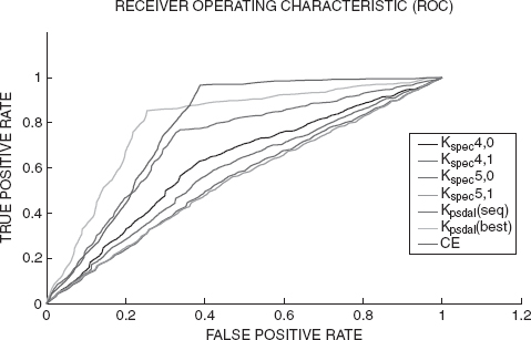
Figure 7.2 shows ROC curves for the spectrum kernels and for other representative kernels–methods used here. The spectrum kernels perform worse than the other methods at all points of the curve. Also, the spectrum kernel with window size 4 performs better than other spectrum kernels at all points on the ROC curve, which complies with the results reported in [49]. Thus, we conclude that the current task is quite difficult for the traditional kernels and the methods developed here outperform them.
7.7 DISCUSSION AND CONCLUSION
This chapter explores construction of kernels on protein structures by combining kernels on neighborhoods. We defined two types of neighborhoods, and kernels on each type of neighborhood, utilizing both sequence and structure information. We also explored two different ways of combining these kernels to get kernels on neighborhoods. The neighborhood kernels were combined in mainly two ways to form kernels on entire protein structures: by adding similarity between all pairs of neighborhoods (Knps), and adding similarity between equivalent pairs of neighborhoods (Knal and psdal). The NPS kernels do not require any structural alignment information while the other kernels require structural alignment.
Experiments conducted on the well-known structural classification benchmark SCOP [12] show that the alignment kernels perform reasonably accurately on the difficult task of classifying 40% sequence nonredundant data set. Some of them also outperformed the well known structural alignment program CE [21]. Thus, the kernels developed here can be useful for real-life bioinformatics applications.
Various experiments with the kernels confirmed that they behave predictably with respect to various parameters. For example, in Section 7.4.2, it was predicted that decreasing the values of β and σ will increase the classification accuracy to a point where numerical errors start reducing them. It was validated by experimental results in Section 7.6.4. Also, as expected, structural information was found to be more effective for the current task than sequence information.
The NPS kernels are designed from basic principles to capture structure and sequence information in proteins, and do not require any structural alignment. This approach is in contrast with the approach taken in [16], which essentially tries to make a positive semidefinite kernel out of the MAMMOTH similarity score. In spite of these advantages, NPS kernels have high computational complexity and are not very accurate. An interesting problem is to improve the accuracy of such kernels without increasing the time complexity. Another interesting approach could be to train a probabilistic model for protein structures and define fisher kernels [6] on the same.
The Knps were shown to be analogous to the spectrum kernels in the sense that when restricted to use only sequence information, they turned out to be the normalized versions of the spectrum kernels. However, while the neighborhood pair sum kernels do not perform as well as the structure alignment algorithms (CE), the spectrum kernel is reported to be performing comparably with the sequence alignment algorithms (e.g., BLAST or Smith–Waterman [49]).
We have defined various sequence based kernels on neighborhoods, following various interpretations of the sequence neighborhoods (e.g., sets, strings, structures, etc.). However, not much variation was observed in performance of each of these types of kernels. The reason for this is that sequence information is not sufficient for achieving good accuracy on the current task. It will be interesting to see how these sequence based kernels on neighborhoods fare on different types of sequence processing tasks, when combined in a manner analogous to the ones described in this chapter.
In summary, we have described neighborhood based kernels, which form a reasonably broad class of kernels. Even though the kernels described here were designed for protein structures, we believe the same design principles can be applied to design kernels on general attributed pointsets [10].
APPENDIX A
A substructure ![]() of protein PA centered at residue i is a set of l residues that are closest to residue i in 3D space, l being the size of substructures being considered. Thus,
of protein PA centered at residue i is a set of l residues that are closest to residue i in 3D space, l being the size of substructures being considered. Thus, ![]() . The robust algorithm for comparing protein structuresPA and PB is
. The robust algorithm for comparing protein structuresPA and PB is
1. Compute the substructures centered at each residue for both proteins PA and PB.
2. For each pair of substructures, one from each protein, compute the alignment between the substructures by solving the problem described in Eq. 7.6).
3. For each substructure alignment computed above, compute the optimal transformation of the sub-structure from PA onto the one from PB. Transform the whole of PA onto PB using the computed transformation, and compute the similarity score between residues of PA and PB.
4. Compute the optimal alignment between PA and PB by solving the assignment problem using the similarity score computed above.
5. Report the best alignment of all the alignments computed in the above step as the optimal one.
The substructure-based algorithm relies on the assumption that the optimal structural alignment between two protein structures contains at least one pair of optimally and fully aligned sub-structures, one from each of the proteins. For each substructure alignment computed in step 2 above, the optimal transformation superposing the corresponding residues is calculated using the method described in [31]. The “best” alignment mentioned in step 5 is decided on the basis of both RMSD and the length of alignment. A detailed description and benchmarking of the method will be presented elsewhere.
REFERENCES
1. J. Shawe-Taylor and N. Cristianini (2004), Kernel Methods for Pattern Analysis. Cambridge University Press.
2. L. Wolf and A. Shashua (2003), Learning over sets using kernel principal angles. J. Mach. Learning Res., (4):913–931.
3. R. Kondor and T. Jebara (2003), A kernel between sets of vectors. Tom Fawcett, Nina Mishra, Tom Fawcett, and Nina Mishra (Eds.), ICML, AAAI Press, pp. 361–368.
4. A. Shashua and T. Hazan (2005), Algebraic set kernels with application to inference over local image representations. Lawrence K. Saul, Yair Weiss, and Léon Bottou (Eds.), Advances in Neural Information Processing Systems 17, MIT Press, Cambridge, MA, pp. 1257–1264.
5. C. Leslie and R. Kwang (2004), Fast string kernels using inexact matching for protein sequences, J. Mach. Learning Res., 5:1435–1455.
6. T. Jaakkola, M. Diekhaus, and D. Haussler (1999), Using the fisher kernel method to detect remote protein homologies. 7th Intell. Sys. Mol. Biol., pp. 149–158.
7. L. Holm and C. Sander (1996), Mapping the protein universe. Science, 273(5275):595–602.
8. I. Eidhammer, I. Jonassen, and W. R. Taylor (2000), Structure comparison and structure patterns. J. Computat. Biol., 7(5):685–716.
9. H. J. Wolfson and I. Rigoutsos (1997), Geometric hashing: An overview. IEEE Comput. Sci. Eng., 4(4):10–21.
10. M. Parsana, S. Bhattacharya, C. Bhattacharyya, and K.R. Ramakrishnan (2008), Kernels on attributed pointsets with applications. In J.C. Platt, D. Koller, Y. Singer, and S. Roweis (Eds.), Advances in Neural Information Processing Systems 20, Cambridge, MA, MIT Press, pp. 1129–1136.
11. S. Bhattacharya, C. Bhattacharyya, and N. Chandra (2007), Comparison of protein structures by growing neighborhood alignments. BMC Bioinformat., 8(77).
12. A. G. Murzin, S. E. Brenner, T. Hubbard, and C. Chothia (1995), Scop: a structural classification of proteins database for the investigation of sequences and structures. J. Mol. Biol., 247:536–540.
13. C. A. Orengo, A. D. Michie, S. Jones, D. T.-Jones, M. B. Swindells, and J. M Thornton (1997), Cath- a hierarchic classification of protein domain structures. Structure, 5(8):1093–1108.
14. J.-P. Vert, H. Saigo and T. Akutsu (2004), Kernel Methods in Computational Biology, chapter Local alignment kernels for biological sequences, MIT Press, MA, pp. 131–154.
15. K. M. Borgwardt, C. S. Ong, S. Schauer, S. V. N. Vishwanathan, A. J. Smola, and H.-P. Kriegel (2005), Protein function prediction via graph kernels. Bioinformatics, 21 Suppl. 1:47–56.
16. J. Qiu, M. Hue, A. Ben.-Hur J. P. Vert, and W. S. Noble (2007), A structural alignment kernel for protein structures. Bioinformatics, 23:1090–1098.
17. C. Wang and S. D. Scott (2005), New kernels for protein structural notif discovery and function classification. International Conference on Machine Learning.
18. S. Bhattacharya, C. Bhattacharyya, and N.R. Chandra. Structural alignment based kernels for protein structure classification, 24th International Conference on Machine Learning (ICML), 2007.
19. D. Haussler (1999), Convolution kernels on discrete structures. Technical report, University of California, Santa Cruz.
20. S. Bhattacharya, C. Bhattacharyya, and N. Chandra (2006), Projections for fast protein structure retrieval. BMC Bioinformat., 7 Suppl.:5S–S5.
21. P. E. Bourne and I. N. Shindyalov (1998), Protein structure alignment by incremental combinatorial extension of optimal path. Protein Eng., 11(9):739–747.
22. B. Scholkopf and A.J. Smola (2002), Learning with Kernels. MIT Press, MA.
23. T. Hofmann, B. Scholkopf, and A. J. Smola (2007), Kernel methods in machine learning. Technical report, arXiv, Avialble at (http://arxiv.org/abs/math/0701907v1).
24. M. Collins and N. Duffy (2001), Convolution kernels for natural language. Advances in Neural Information Processing Systems, MIT Press, Cambridge, MA. pp. 625–632.
25. S. V. N. Vishwanathan and A. Smola (2005), Binet-cauchy kernels. In Lawrence K. Saul, Yair Weiss, and Léon Bottou, editors, Advances in Neural Information Processing Systems 17, MIT Press, Cambridge, MA, pp. 144–448.
26. C. Cortes, P. Haffner, and M. Mohri (2004), Rational kernels: Theory and algorithms. J. Mach. Learning Res., (5):1035–1062.
27. R. Kondor and J. Lafferty (2002), Diffusion kernels on graphs and other discrete structures. Proceedings of International Conference on Machine Learning (ICML).
28. H. Kashima, K. Tsuda, and A. Inokuchi (2003), Marginalized kernels between labeled graphs. Proceeding of the Twentieth International Conference on Machine Learning, AAAI Press, pp. 321–328.
29. K. M. Borgwardt and H.-P. Kriegel (2005), Shortest-path kernels on graphs.
30. In ICDM ‘05: Proceedings of the Fifth IEEE International Conference on Data Mining, Washington, DC, 2005. IEEE Computer Society, pp. 74–81. T. Horváth, T. Gärtner, and S. Wrobel (2004), Cyclic pattern kernels for predictive graph mining. KDD ‘04: Proceedings of the tenth ACM SIGKDD international conference on Knowledge discovery and data mining, ACM, NY, pp. 158–167.
31. B. K. P. Horn (1987), Closed form solution of absolute orientation using unit quaternions. J. Opt. Soc. Am., 4(4):629–642.
32. L. Holm and C. Sander (1993), Protein structure comparison by alignment of distance matrices, J. Mol. Biol., 233:123–138.
33. S. Umeyama (1988), An eigendecomposition approach to weighted graph matching problems. IEEE Trans. Pattern Anal. Mach. Intell., 10(5):695–703.
34. D. Bertsimas and J. Tsitsiklis (1997), Introduction to Linear Optimization. Athena Scientific.
35. J. Shapiro and D. Brutlag (2004), Foldminer: Structural motif discovery using an improved superposition algorithm. Protein Sci., 13:278–294.
36. S. F. Altschul W. Gish, W. Miller, E. W. Myers, D. J. Lipman (1990), Basic local alignment search tool. J. Mol. Biol., 215(3):403–410.
37. S. Henikoff and J.G. Henikoff (1992), Amino acid substitution matrices from protein blocks. Proc. Natt. Acad. Sci., 89:10915–10919.
38. G. R. G. Lanckriet, N. Cristianini, P. Bartlett, L. El Ghaoui, and M. I. Jordan (2004), Learning the kernel matrix with semidefinite programming. J. Mach. Learning Res., 5:27–72.
39. F. R. Bach, G. R. G. Lanckriet, and M. I. Jordan (2004), Multiple kernel learning, conic duality, and the smo algorithm. ICML ‘04: Proceedings of the twenty-first international conference on Machine learning p. 6, ACM. New York, NY.
40. K. Tsuda (1999), Support vector classifier with asymmetric kernel functions. European Symposium on Artificial Neural Networks (ESANN), pp. 183–188.
41. B. Schölkopf, J. Weston, E. Eskin, C. S. Leslie, and W. S. Noble (2002), A kernel approach for learning from almost orthogonal patterns. ECML, 511–528.
42. D. Greene and P. Cunningham (2006), Practical solutions to the problem of diagonal dominance in kernel document clustering. ICML’ 06: Proceedings of the 23rd international conference on Machine learning, ACM, NY. pp. 377–384.
43. M. Novotny, D. Madsen, and G. J. Kleywegt (2004), Evaluation of protein fold comparison servers. PROTEINS: Struct., Function, and Bioinformat., 54:260–270.
44. E. Anderson, Z. Bai, C. Bischof, S. Blackford, J. Demmel, J. Dongarra, J. Du Croz, A. Greenbaum, S. Hammarling, A. McKenney, and D. Sorensen (1999), {LAPACK} Users’ Guide. Society for Industrial and Applied Mathematics, 3rd ed., Philadelphia, PA.
45. C.-C. Chang and C.-J. Lin (2001), {LIBSVM}: a library for support vector machines, Available at http://www.csie.ntu.edu.tw/∼cjlin/libsvm.
46. J. M. Chandonia, G. Hon, N. S. Walker, L. Lo Conte, P. Koehl, M. Levitt, and S. E. Brenner (2004), The astral compendium in 2004. Nucleic Acids Res., 32:D189–D192.
47. G. Wang and R. L. Dunbrack (2003), Pisces: a protein sequence culling server. Bioinformatics, 19(12):1589–1591.
48. F. J. Provost and T. Fawcett (2001), Robust classification for imprecise environments. Mach. Learning, 42(3):203–231.
49. C. S. Leslie, E. Eskin, A. Cohen J. Weston, and W. S. Noble (2004), Mismatch string kernels for discriminative protein classification, Bioinformatics, 4:467–476.