CHAPTER 14

TECHNIQUES FOR PRIORITIZATION OF CANDIDATE DISEASE GENES

JIEUN JEONG AND JAKE Y. CHEN

14.1 INTRODUCTION

Gene prioritization is a new approach for extending our knowledge about diseases and phenotypic information each gene encodes. We will review computational methods that have been described to date and attempt to identify which are most successful and what are the remaining challenges. The motivations and applications of this topic been well described in [1]. Therefore, we focus on how to enable a biologist to select the best existing method for a given application context. At the same time, we would like to identify remaining open research problems for practitioners in bioinformatics.

The general notion of gene prioritization assumes that one has a set of candidates and he wants to order the candidates from the most promising to the least promising one. A primary motivation for prioritization of candidate disease genes comes from the analysis of linkage regions that contain genetic elements of diseases. In this setting, the notion of a disease gene is unambiguous: a genetic element that confers disease susceptibility if its variants is present in the genome. For a particular disease phenotype, researchers often have a list of candidate genes usually genes located in a linkage interval associated with the disease. Finding the actual gene and candidate can be a subject of expensive experimental validations; however, once identified as real, these disease-associated genes or their protein products can be considered as a therapeutic target or a diagnostic biomarker. Online Mendelian Inheritance in Man (OMIM) is a representative database that links phenotypes, genomic regions, and genes. Here, we refer to a “phenotype” as a disease phenotype. To make effective use of biological resources, computational gene prioritization allows researchers to choose the best candidate genes for subsequent experimental validations.

The ultimate goal of gene prioritization is to find therapeutic targets and diagnostic biomarkers, the notion of a disease-related gene can be more general, i.e., a gene or a protein involved in the disease process either directly or indirectly. In turn, the list of candidates can originate from many data sources, e.g., genome-wide association studies serial analysis of gene expression (SAGE), massively parallel signature sequencing (MPSS) [2], or proteomic experiments. Such prioritization can be applied to either a short list of genes or the entire genome [3].

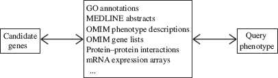
Disease gene prioritization requires researchers to take advantage of prior knowledge about both genes and phenotypes. We assume that “the truth is always there”, which is embedded in large volumes of potentially relevant publications and various tabulated results from high-throughput experiments. A computational disease-gene prioritization method should be able to convert this data into insights about the relationship between candidate genes and interested disease phenotypes (see Fig. 14.1

The first work on prioritization of candidate genes from linkage regions [4,5] used text mining to extract phenotype descriptions and establish similarities among phenotypes and the relationships between phenotypes and genes. The underlying assumption is that a good candidate gene with a strong connection to the query phenotype, i.e., phenotype under investigation, can be identified by sifting through biomedical literature. Text mining allows more high-throughput scanning of the biomedical literature to develop credible content; therefore, it can be less costly than curation-based database development, e.g., LocusLink and RefSeq [6], GO (Gene Ontology) [7], and OMIM [8]. In Section 14.2, we will review gene prioritization methods and related databases that are developed based on biomedical text mining.

Both literature curation and text mining based approaches extract relationships between phenotypes and genes, all based on biological and biochemical processes that have been already identified. Thus, a pontential drawback is that genes that are less well characterized can be overlooked. Such “blind spot” can be targeted by complementary methods that do not rely on properties of phenotypes, e.g., lists of known disease genes or text-mined associations. One class of such complementary methods reported was to identify general properties of genomic sequences of disease genes [9–11] and relate genes from different loci (or linkage regions) of the same phenotype [12]. These methods will be reviewed in Section 14.3.

With the arrival of systems biology, several recent emerging methods have used data on biomolecular interactions among proteins and genes, most notably protein–protein interactions, biological pathways, and biomolecular interaction networks (see [13–19]). In Section 14.4, we will review different ways of gene prioritization based on interaction networks.

In Section 14.5, we describe how gene prioritization can be obtained with a unified phenotype-gene association network in which gene–gene links are taken from biomolecular interaction networks and phenotype–phenotype links are identified with results from text-mining.

One difficulty in prioritizing disease genes is the lack of data on many possible gene candidates. For example, among roughly 23,000 identified human genes, only 50–55% have GO annotations, which suggests that for the remaining genes we do not know about their biological processes, cellular components, or molecular functions. Networks of biomolecular interactions cover a similarly small percentage of genes. Gene expression data, on the other hand, can cover many genes that are otherwise uncharacterized genomic DNA. Using data of many types, especially high-throughput experimental and computational-derived data, has the potential to improve the quality of gene prioritizations that leads to new discoveries. However, the inherent “noisy” nature of high-throughput experimental data and computationally derived data raise the question how to combine different sources of data so that the integrated data improves the predictive power of gene prioritizations. We refer to this problem as the challenge of data fusion problems in gene participations and will describe different solutions in Section 1.6.

14.2 PRIORITIZATION BASED ON TEXT-MINING WITH REFERENCE TO PHENOTYPES

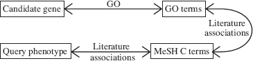
Perez-Iratxeta et al. [5] developed a method that uses the MEDLINE database and GO data to associate GO terms with phenotypes. Then, they ranked the candidate genes based on GO terms shared with the query phenotype. Later, they implemented this strategy as a web application [20]. The phenotype-GO term association was derived using MeSH C terms (medical subject headings from chemistry recognized in MEDLINE queries): An article stored in MEDLINE that mentions both terms creates an association pair. They measured the strengths of associations between phenotypes and MeSH C terms and between MeSH C and GO terms, and used a “max-product” rule from fuzzy logic to obtain the strength of the relationship between phenotypes and GO terms. The relationship GO term gene also has “strength” (which takes larger values for less frequent terms) and the same max-product rule can define the strength of the gene-phenotype relationship. Then, this “strength” was taken as the priority score (see Fig. 14.2. Clearly, this methods allow the aggregation of different relationships between specific phenotypes and genes to identify additional information absent in biomedical texts separately. For example, one article evaluates effectiveness of a drug (MeSH C term) in the treatment of a phenotype, and another, the impact of that drug on a metabolic process (GO term). The enrichment on “artificial linkage regions” was approximately 10-fold, i.e., locating the correct candidate in the top 5% half of the time.

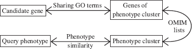
Freudenberg and Propping [4] used an different version of chain of associations (see Fig. 14.3). They defined between disease phenotypes a similarity score that was based on five key clinical features and clustered the phenotypes from OMIM according to the score. The OMIM also provides associations of phenotype-genetic cause, and this defines the last step in their chain. The enrichment reported in this article is similar to Perez-Iratxeta et al. [5].

van Driel et al. [21] developed a tool that could “data mine” up to nine web-based databases for candidate genes and could be used to select “the best” candidates in a linkage region. The user can specify a genomic region, which can be a linkage region, and a set of anatomic terms that describe the localization of symptoms of a Mendelian disorder provided by the user. The result gives two lists of genes from the genomic region: those that were found in at least one tissue from the set (OR list) and those that were found in all tissues from the set (AND list). The count of lists in which a gene is present can be viewed as a priority with possible values, 0, 1, or 2; in ten examples of diseases used in this chapter, they determined an average enrichment (the correct candidate was always present in the OR list). The localization of disease symptoms and the tissue localization of a disease-related protein is apparently an important part of “prior knowledge”, but it is not apparent how to choose the best anatomic terms for a particular phenotype. Tiffin et al. [2] developed a method to make this decision “automatic”. They used eVOC vocabulary of anatomic terms that is hierarchically organized like GO with only the “part of” relationships (e.g., retina is a part of eye). Applying text-mining, they counted MEDLINE papers that mention both the disease and the particular eVOC term. A term was counted as being present in a paper if its hypernym was present. These measures were then used to represent the strength of associations of phenotypes with anatomic terms. They obtained similar association of eVOC terms with genes. Then, each phenotype and each gene had its list of “n most significant eVOC terms.” Finally, the number of terms that occur both in the list of a candidate gene and in the list of the query phenotype is the inferred priority for genes.

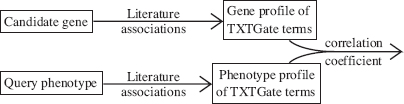
Both Perez-Iratxeta et al. [5] and Tiffin et al. [2] used the concept of chains of associations with different computational algorithmic flavors. Several recent papers used Pearson correlation of profile vectors. For example, Aerts et al. [22] used the MEDLINE database of abstracts in conjunction with the TXTGate vocabulary [23], which was developed specifically for gene analysis. A profile of “subject” X is a vector with an element for every term t and this element is the over-representation or under-representation or of occurrences of term t in articles that mention X compared with the frequency of occurrences of t in the entire database. Since both genes and phenotypes are “subjects”, one can define the closeness of gene g to phenotype p as the Pearson correlation coefficient of profile(p) and profile(g) (see Fig. 14.4). This method was a component of a more complex prioritization system ENDEAVOUR that will also be discussed in Section 14.6.

14.3 PRIORITIZATION WITH NO DIRECT REFERENCE TO PHENOTYPES

Using literature to find associations between phenotypes and vocabulary terms was successful, but rarely new disease genes can be discovered using those associations. One reason is that many terms important for a given phenotype may not be discussed in articles that mention the phenotype’ in addition, many new disease genes are yet to be annotated.

The POCUS method of Turner et al. [12] addressed the first problem. They applied two types of gene annotations, GO terms and InterPro domains for phenotypes that are associated with multiple genetic loci (linkage regions). The idea is that for such phenotypes one can discover important associations that were not yet reported in the literature. Within a single locus associated with phenotype p, genes with a certain term X (a type of protein domain or with a certain GO annotation) can be over-represented because of tandem duplications that place similar genes next to each other. Therefore, having term X does not identify a disease gene within that locus. However, if a gene g from another locus that is associated with p has term X, it raises the possibility that term X and gene g are significant for the query phenotype p. More precisely, gene g obtains a score because of term X if X also occurs in other loci of Phenotype p, and the score is based on the probability that two loci with a particular number of distinct terms containing the term X.

Turner et al. [12] tested POCUS on 29 phenotypes with multiple loci containing known disease genes, and on one specific disease, autism, which had two new genes discovered during the time of the research by Turner et al. In 11 cases, no disease genes could be identified using this method, due to enforcement of a stringent significance threshold filter. However, but in the remaining 18 cases, the genes that passed threshold filters were considerably enriched with disease genes. In the case of autism, the newly discovered genes were ranked as the best or second best in their artificial linkage region, confirming the future predictive power of such methods.

TOM by Rossi et al. [24] is a web-accessible tool with a “two-loci option” that has exactly the same purpose as POCUS besides. In addition to GO annotations, TOM also uses expression profile similarity.

While POCUS does not rely on prior literature to identify terms that are significant for the query phenotype, it relies on existing GO annotations that are available for approximately 60% of known human genes according to the GO annotation provided by the SwissProt database as well as available InterPro domain annotations. This motivates follow-up work that do not rely on any annotations of the candidate genes. Lopez-Bigas et al. [9] and Adie et al. [10] developed a decision tree method that is based solely DNA sequence features of the candidate gene, such as coding potential for a signal peptide, the similarity with its mouse homolog, the number of exons, and so on. The enrichment of PROSPECTR, the latter version of the approach, is close to 2-fold, i.e., the correct candidate appearing in the top 5% with a frequency of 10%. While modest, this result does not rely on any knowledge except for a DNA sequence. Further development in this direction can be promising in the context of interpretation of results from genome-wide association studies, because in those cases we know not only the DNA sequence, but also the exact type of variations.

14.4 PRIORITIZATION USING INTERACTION NETWORKS

Many methods using interactions in prioritizing candidate genes are fundamentally counting and comparing “qualified” interactions under the following underlying assumptions: 1) causative genes for a disease reside in the same biological module; 2) genes in the module have many interactions with other members within the module and relatively few interactions with nonmembers outside the module.

The observation that disease genes share interactions at a much higher rate than random gene pairs was made when protein–protein interaction (PPI) networks were assembled [25]. In this discussion, we will use some graph terms. A network is a graph composed of a set of nodes (genes as identified with their protein products) and a set of pairs of nodes called edges (that indicate the existence of interactions). If we have an edge u,v, we say that u and v are neighbors. For a node u, N(u) is the set of its neighbors, and for a node set A, N(A) is formed from A by inserting the neighbors of its elements. We will also use T to denote the set of known disease genes for the query phenotype (the training set).

George et al. [26] tested whether a PPI network could be used to propose candidates. They used the OPHID network [9] that consolidates interactions from HPRD, BIND, and MINT, curated networks of interactions that were reported in the literature, as well as results of high-throughput experiments that were performed on human proteins and proteins of four model species (baker’s yeast, mouse, nematode, and fruit fly) that were mapped to their orthologous human proteins. Rather than ranking candidates, George et al. [26] were simply making predictions: any gene in N(T) that is within the investigated linkage interval is a candidate. To test the quality of these predictions, they used a set of 29 diseases with 170 genes, the same set as the set used to test the POCUS method by Turner et al. [12]. This benchmark showed very good performance: 42% of the correct candidates were identified and no incorrect candidates were identified.

The work of Oti et al. [27] drew quite different conclusions. They compared the gene prioritization results based on two networks: (1) HPRD (assembled by Gandhi et al. [28], a curated collection of 19,000 PPIs based on the literature and (2) a network expanded with results of high-throughput experiments on human proteins and three model species. They tested the same prediction method as George et al. [27] on 1114 disease loci for 289 OMIM phenotypes that shared at least two known disease genes. This led to 432 predictions, 60% of which based on HPRD were correct as compared with 12% of which based on high-throughput data were correct. These results revealed the challenge even though biomolecular interactions may generate most trustworthy predictions, the number of such high-quality predictions is dependent on the coverage of PPI, which is still quite poor today. To make more predictions, we need to use some combination of (a) a larger network, (b) indirect interactions, and (c) methods that prioritize candidates that have these indirect connections. Otherwise, one must explore how to use prior knowledge to expand set T. In tests conducted by Oti et al. [27], the average size of T was 2, while in tests of George et al. [26], this size was more than twice as large at 4, a major motivation for the methods that we will discuss in Section 14.5.

Aerts et al. [22] used ranking based on PPI as one of the components of their ENDEAVOR program. They used the BIND PPI network developed by Bader et al. [27], which is similar to the expanded version of the network used by Oti et al. [27]. Using graph definitions, the priority score for a gene u is the count of its neighbors in (N(T)). They subsequently order the candidate list from the largest to the smallest priority score. Here, each of the points (a–c) is addressed. However, the formula for the priority value does not take into account of very high variability of numbers of neighbors of nodes in the PPI graph, which varies between 1 and >1000. Clearly, being a neighbor of a node with degree 1 provides a much more specific hint of relatedness than being a neighbor of a node with degree 1000.

Franke et al. [29] used several data sources, but they also evaluated the use of an interaction network that had a large majority of interactions from the BIND PPI network, with a small number of coexpression-based “interactions” added (the MA+PPI data set). Their priority function is described as an empirical p-value of kernel scoring function of the shortest path distance from node u to T, but a much simpler definition defines the same ranking. If d(u,T) is the distance (defined as the shortest path length) from u to T and there are k network nodes that are not further from u than d(u,T), then they effectively use k as the priority value of u and they rank candidates from the smallest to the largest priority value. When they used MA+PPI only, the correct candidates appeared at the top 5 (of 100) candidates 8% of the time, hence they concluded that MA+PPI “lacks predictive performance”.

The above methods are based on basic graph concepts and all are rooted in the notion of path distance in the network graph. However, measures derived from graph distance can be misleading. As we mentioned, one issue is the wide range of the numbers of neighbors that different nodes have. Moreover, disease genes are not a representative sample of all genes as they tend to have more interactions than the average. To address these issues, Aerts et al. [22] have a priority formula that is “much easier” for proteins with many interactions (network hubs) than for others, conversely, the formula of Franke et al. [29] eliminates that advantage. Which is the correct approach? Or perhaps there is a “third approach” that can avoid the pitfalls of either extreme position?

Indeed, a much more successful method was introduced recently by Köhler et al. [30]. They proposed a more elaborate network-based prioritization method based on global distance measure in the application of finding disease genes from linkage analysis. They also compared their methods with the methods based on local distance measures [26,27] and ENDEAVOUR [22] to show that their own methods performed better.

A physical example of global distance would be a resistance between two points of an electric network; computing such resistance with Kirchoff’s circuit law requires us to know the entire network. We can also talk about “closeness”: If we apply some positive voltage to the first point and ground to the second point, the closeness would be the resulting current. Köhler et al. [30] discussed two global distance measures, random walk with restart (RWR) and diffusion kernel. In evaluation, diffusion kernel leads to very similar results as RWR; computationally and conceptually, these methods are quite similar, so we will describe RWR only here. The general concept of these methods is to start a random walk by selecting a node in set T and use the rules of the walk to compute the stationary probability distribution of the position of the walker. A good set of rules should assure that this probability measures closeness, or relatedness, of various positions to set T, so we can rank the candidate genes based on those closeness scores.

In RWR, the random walker first decides if it should continue the walk (with probability 1-r) or to restart (with probability r). In the former case, it changes its position from the current node c to a randomly selected neighbor in N(c); in the latter, it “jumps” to a random node in T.

To describe RWR more precisely, we will use W to denote the column-normalized adjacency matrix of the network and pt to denote a vector in which the ith element holds the probability of the walker being at node i at time step t. The walker starts by moving to each disease gene (a node in T) with probability 1/|T|, so the ith element of p0 is 1/|T| if i is in T and 0 otherwise. Then, at each time step t, the random walker has probability r to restart (i.e., to repeat the starting move) and with probability 1-r the random walker chooses to follow an edge from its current node, each edge with the same probability. This defines the simple update rule of how to change the probability distribution of the location of the walker, namely, p changes to rp0+(1-r)Wp (i.e., pt+1 = rp0+(1-r)Wpt). They repeat this update until the sum of changes of the elements of p becomes <10-6, so that p becomes a good approximation of the steady-state distribution. The final probabilities of each node are the priority values and the ranking is from the largest to the smallest value.

For comparison with other methods, Köhler et al. [30] implemented direct interactions (DI) with other known disease-family genes and single shortest path (SP) to any known disease gene in the family. They computed results for 110 phenotypes with 783 known disease genes using a “1-out, artificial linkage region of 100” approach (the same approach as [22,26,29]). They tested the results on their screens of candidate genes in an artificial linkage interval, i.e., the prediction of gene g tested by removing g from T and considering a set S of 100 candidate genes that flank g in two directions on the chromosome. They also ranked genes in S with PROSPECTR, which is based on sequence-based features, and with ENDEAVOUR, which is based on several different types of data. Both mean-fold enrichment and ROC analysis showed that their methods perform much better than the other methods they were compared with.

The shortest path method, was considered by George et al. [26], but as we mentioned before, they merely tested predictions made when the shortest path has length 1, i.e., they did not test the ranking based on SP length. Correct predictions were made in 42% of the tested artificial linkage intervals where they did not observe incorrect predictions. In 61% of the cases in the tests of Köhler et al., where the approach of George et al. [26] and Oti et al. [27] yielded a correct prediction, some genes are also predicted incorrectly. An analogous situation, multiple nodes having the best priority value, is very rare for the RWR method: of the cases when the correct candidate had the top score, only 1.4% had another node within the investigated linkage interval with the same score. Moreover, RWR assigns a top score to the correct candidate more often. Thus, one of the advantages of RWR is that when SP selects several genes with the same score, RWR usually correctly picks a single good candidate. The measure for the assessing the quality of a method developed by Köhler et al., mean enrichment, can be explained as follows: if the evaluated candidate gets rank a, we score it as enrichment 50/a, and we calculate the mean. For example, if the evaluated gene always receives a rank between 1 and 5 (out of 100 possible ranks) with equal probability, this gives mean enrichment of (50/1+ 50/2+50/3+50/4+50/5)/5 = 22.8. The mean enrichment for RWR was 26, and for SP and DI it was 18. They also tested various methods on seven recently identified disease genes and the mean enrichment for RWR and SP was 25.9 and 17.2, respectively. They also obtained ENDEAVOUR ranks for those genes and the resulting mean enrichment was 18.4. This is very intriguing because ENDEAVOUR presumably considers many data sources and obtained top evaluations in other papers. Apparently, many biases and coverage issues can confound literature or data integration based gene prioritization methods but may be addressed with the use of biomolecular interaction networks.

14.5 PRIORITIZATION BASED ON JOINT USE OF INTERACTION NETWORK AND LITERATURE-BASED SIMILARITY BETWEEN PHENOTYPES

One conclusion from the results of Köhler et al. [30] concerning the effectiveness of their RWR ranking method could be that PPI interactions alone can provide the best possible prediction of disease genes. This conclusion may be premature, because RWR was tested on phenotypes that on average had seven known disease genes. The comparison of results of George et al. [26] and Oti et al. [27] suggests that the reliability of a method based on PPI interactions may decrease as the number of known disease genes decreases. Moreover, for roughly one-third of the phenotypes in OMIM, there are no known disease genes, and in these cases PPI methods described in Section 14.4 cannot be applied at all. However, even if no disease genes are identified for a given phenotype, we have considerable prior knowledge in the form of (1) knowledge that phenotypes are similar and (2) accumulated knowledge about the similar phenotypes.

The notion of similarity of phenotypes was used first by Freudenberg and Propping [4], who defined a measure of “closeness” for phenotypes and computed phenotype clusters as the initial stage of their prioritization method. One could simply combine that approach with, for example, RWR. Given a phenotype compute its cluster, and then use the set T that consists of all known disease genes of all members of the cluster. This requires making an arbitrary decision on whether to cluster the phenotypes or avoid clustering with the use of phenotype–phenotype similarity.

Most gene prioritization methods integrate two different types of data: literature-based data and interactome data [3,31]. They use similarities between phenotypes based on literature curation and the interaction network, and are guided by the assumption that causative genes for the phenotypically similar diseases reside in the same biological module. In turn, a biological module corresponds to a fragment of the network that contains many interactions.

To justify that assumption, Lage et al. [31] described a situation when a protein complex is vital to some biological process, while mutations of genes of the proteins that participate in that complex have a negative impact on that process leading to diseases with different, but related symptoms. Therefore, connections in PPI network between the constituents of the complex are reflected in similarities between phenotypes that are related to their genes. Alternatively, there can be biological pathways with similar consequences: disease proteins have many interactions among themselves, which make up the basic assumption for all network-based prioritization methods. Lage et al. [31] identified so-called “disease complexes” for each candidate gene and each such disease complex can be seen as a small module (and a disease pathway would be a larger module). They made a unified network of genes and phenotypes where connections between genes were from a PPI network, each with its reliability score, and disease genes were connected to their respective phenotypes while phenotype–phenotype connections were annotated with similarity scores. Then they converted the unified network into a Bayesian network by computing posterior probability for each gene. Intuitively, those probabilities measure the strength of the following tendency: If one moves from the network node of the candidate gene to its network neighbors and then to the phenotypes (if any) associated with those neighbors, he can arrive at a phenotype that is similar to the query phenotype. Consequently, the posterior probabilities of genes define their priority values.

Following this work, Wu et al. [3] also proposed the prioritization method based on the same assumption as Lage et al. [31], but much simpler. In addition to the general assumption of all network-based prioritization methods, they made the following assumption for their method called “CIPHER,” in which members of a disease module have positive correlation of gene–gene relatedness and phenotype–phenotype similarity while nonmembers lack such correlation. They also tested the levels of these correlations to predict module members. Their method can be described as the sequence of the following steps:

First, for the query phenotype p, collect similarity scores (described at the end of this section) to all other phenotypes in the phenotype–gene network. This forms a vector profile(p).

Second, for a pair of candidate gene g and phenotype q, define closeness(g,q) as the number of neighbors of g that are disease genes of q. By collecting these values for all q’s we obtain a vector profile(g).

Third, the priority value of g is the Pearson correlation coefficient of profile(g) and profile(p). The gene with the highest value receives the rank of the top candidate.

They compared this method with other methods including those by Freudenberg and Propping [4], Gaulton et al. [32], and ENDEAVOR. They determined that their methods perform much better than the first two methods and have comparable performance with ENDEAVOR. A direct comparison of CIPHER with RWR of Köhler et al. [30] is not simple because Wu et al. use a different set of test cases and a different definition of enrichment. In both methods, when applied to artificial linkage intervals of size 100 (109 for CIPHER) in “leave-one-out” manner, the correct candidate had the top rank roughly 50% of the time. The additional strength of CIPHER is revealed using “leave-all-out” tests in which we remove the knowledge of all gene-disease associations for the query phenotype. The performance in those tests was only somewhat weaker than in “leave-one-out” tests. The explanation is that CIPHER uses the associations of genes with the remaining phenotypes and similarities of those phenotypes with the query phenotype. A weakness of CIPHER is its inability to prioritize genes with no known interactions with disease genes or where there is no single connected interaction network. A modification of CIPHER called CIPHER(SP) alleviated the limitation because it computes closeness(g,q) using profiles of disease genes of q and the shortest path distances from g to those genes. However, CIPHER(SP) performs worse than CIPHER. This is not surprising given the results of Köhler et al. [30], in which the shortest path distance should probably be replaced with some version of global distance. Therefore, one can expect that a “fusion” of RWR and CIPHER would have wider applicability and superior performance to either of these methods.

Of special note is the concept of phenotype similarity, which was widely used [3,4,31,33]. Freudenberg and Popping [4] measured the similarity between disease phenotypes from the OMIM database using five indices, i.e., episodic, etiology, tissue, onset, and inheritance. They gave simple similarity scores for the pairs of diseases by comparing the individual indices. van Driel et al. [33] developed a text analysis technique to extract phenotypic features from OMIM to quantify the overlap of their OMIM descriptions. They defined a vector of phenotypic features in OMIM descriptions of phenotype p by mining terms from the MeSH vocabulary and for each term they counted its occurrences (including its hypernyms) in the text. Thus each term has a value in the feature vector and the similarity between two phenotypes is computed as the cosine of the feature vectors of two phenotypes. Note that this type of feature vector of phenotype p is similar to the profile(p) used by Aerts et al. [22] described in Section 14.2. This method was adapted and refined in Wu et al. [3] and Lage et al. [31].

14.6 FUSION OF DATA FROM MULTIPLE SOURCES

Each prioritization method uses several data sources that allow us to define associations that connect genes, phenotypes and other objects, on which we can compute a priority score. Adding more data sources might yield more reliable results. In particular, each source represents only a partial knowledge and potentially can complement each other to piece together a global view of the knowledge context.

This creates two challenges. First, each data source has to be incorporated in a coherent prioritization framework. Second, one need to develop an integrated formula. Typically, a single prioritization formula uses several but rarely all of these data sources, e.g., associations between genes and phenotypes from OMIM, associations between phenotypes and scientific terms from text mining in MEDLINE abstracts, and associations between genes or proteins from molecular interaction network. However, when one add new data source and associations with another type of data the problem of incorporating mixed data types looms large.

Rossi et al. [24] proposed solving this problem by defining “filters” for the candidate genes. They considered a set of candidate genes and another set of genes as the training set T (as defined in Section 14.4). Genes in T are presumed to be related to the query phenotype either by being explicitly provided by a database like OMIM or obtained in the same way as in the POCUS method, which we discussed in Section 14.3. Then, they use a data source to compute the distance of candidate genes to T. If the data source is GO, they measure the statistical significance of sharing GO terms with the training set. If the data source is the transcriptome data from public repositories, each gene has a vector of expression values, and a candidate gene has a statistical significance of the closeness of its vector to the vectors of genes in T. In this fashion, each candidate gene has two priority scores. Finally, they selected candidates for which both priority values exceed a certain threshold, and they describe them as genes that passed through two filters. This certainly raises the concern that a candidate could be identified by one data source and disqualified by the other due to the incompleteness of the data. This problem is solved by allowing the user of the system to select which filters they want to apply. Clearly, this would be inadequate if we would consider a large number of data sources.

Aerts et al. [22] designed a modular prioritization system, ENDEAVOUR, which uses a large number of data sources and produces a “synthetic” rank. They defined 10 priority scores based on a variety of data sources. Their prioritization process consisted of four steps: (1) compute priority values according to each data source, (2) convert these priorities to ratio ranks, (3) use vectors of 10 ratio ranks to compute values of a summarizing statistic, and (4) use the values of the summarizing statistic as the final priority score.

Several different methods are used in step (1). As we described in Section 14.2, they used “literature” data to represent each gene as a “profile vector” of strengths of associations of a gene with scientific terms, and Pearson correlation coefficient to measure the closeness of a candidate gene to the training set of genes. This vector methodology was used with two other data sources. One type of vector gives expression levels of a gene in 79 human tissues a the gene expression data set. Another type gives for each position a weight matrix of a transcription factor from the TRANSFAC database the best score recorded for that matrix in the cis-regulatory region of the gene.

Four data sources were treated as attributes and in those cases they compute p-values of sharing attributes with the training set in a similar manner to Rossi et al. [24]. Some of the attributes were straightforward, including GO terms, InterPro protein domains, and membership in KEGG pathways. Expression levels of a gene in human tissues can also be treated as attributes because in a dbEST library of a particular tissue, a gene is categorized as present or absent (based on the levels of its ESTs).

Two data sources define priority scores rather directly. One is the minimum e-value of a BLAST alignment of a candidate gene with the genes of the training set. The second is based on the scores of positional weight matrices of transcription factors in the cis-regulatory region of a candidate gene; however, rather than creating the profile for all transcription factors, in this variant, five most significantly ranked transcription factors are established for the training set and the total score that these five give for a candidate gene are simply added up.

The third data source is the graph of a PPI network, which we described already in Section 14.4.

Each candidate gene obtains a vector of 10 priority scores. In step (1), each priority score is replaced with its ratio rank. If there are n candidate genes being evaluated and a gene g has a bth best value, the ratio rank is b/n.

The summarizing statistic computed in step (3) is Q statistic proposed in the biological context by Stuart et al. [34]. Finally, the genes are ranked–ordered according to their values of Q statistic.

A nonstatistician can be puzzled why the Q statistic of n ranks is superior to a sum or a product of those ranks but the evaluation of the method is quite revealing. It is difficult to translate the sensitivity–specificity curves of Aerts et al. to enrichment measures described earlier, but Wu et al. [3] reported ENDEAVOUR to be the “best other method”, based on their evaluations of CIPHER and a similar comparison made by Köhler et al. [30]. Among all the data sources included in ENDEAVOUR, literature profiles were most useful when tested on the OMIM phenotypes and GO annotations were most useful when tested on KEGG pathways, but the results were not significantly worse when the most useful data source was excluded. This suggests that the data fusion based on the Q statistic is effective in combining relatively noisy and incomplete data into reliable prediction.

Most compelling evaluation results were derived from the tests on 10 newly discovered disease genes. In three cases, a very good rank (1 or 3) was obtained using literature profiles alone and slightly worse (2, 3, and 4) using a synthetic rank. In both cases, the synthetic rank was drastically better, 1 and 3 and in the remaining cases the synthetic rank was also significantly better.

One can expect that ENDEAVOUR, being modular, will be improved in the future. Its protein–protein interaction component was not reported by the authors as particularly successful and it can be replaced with a better network method like RWR from Köhler et al. [30]. The application of expression data is limited to expression in healthy human tissues and provides two priority scores. The main challenge is to combine data fusion with the phenotype similarity because it would require larger changes in the modular design; one possibility would be to have a fuzzy training set where the disease genes of similar phenotypes would be available with different degrees.

14.7 CONCLUSIONS AND OPEN PROBLEMS

Gene prioritization problems benefited from the development of systems biology. As comprehensive online databases emerged, researchers used them to develop computational tools that offer practical advice to biologists. Apparently, any candidates for genes responsible for a given phenotype or involved in a biological process should be incorporated as prior knowledge (biological context). There has been significant progress in the selection of the most relevant sources of data, in the development of algorithms applied to various types of data, and finally, in the application of methods to combine results derived from different data sources. Many of the resulting methods are readily available to users either as standalone programs or as web services online.

This “success story” is clearly not yet complete. First, it is still an open question what the best way is to handle different data sources. For example, literature data can be text-mined with different controlled vocabularies. Second, one can try to give better weights to different vocabulary terms or to different types of publications. Using data on protein–gene interaction also raises a different set of questions. “What are the best interaction networks to use”? “What are the best algorithms”? “Does the answer depend on application”?

For other types of biological data, these questions are even more relevant for gene prioritizations. How should we use data on transcription regulation? Aerts et al. [22] did not comment how to practically pick “the best one”. While one debates how to develop more effective methods in the future, there are plenty of questions to address even today. How to use information about protein structure? How can we use gene expression data and proteomics data? The list goes on. One thing for sure is that this area will be a subject of many new developments in the near future.

14.8 ACKNOWLEDGMENT

We thank Michael Grobe for reviewing this chapter and giving invaluable comments.

REFERENCES

1. C. Giallourakis, C. Henson, M. Reich, X. Xie, and V. K. Mootha (2005), Disease gene discovery through integrative genomics, Annu. Rev. Genomics Hum. Genet., ED-6: 381.

2. N. Tiffin, J. F. Kelso, A. R. Powell, H. Pan, V. B. Bajic, and W. A. Hide (2005), Integration of text- and data-mining using ontologies successfully selects disease gene candidates, Nucleic Acids Res., EDL-33(5): 1544.

3. X. Wu, R. Jiang, M. Q. Zhang, and S. Li (2008), Network-based global inference of human disease genes, Mol. Syst. Biol., ED-4: 189.

4. J. Freudenberg and P. Propping (2002), A similarity-based method for genome-wide prediction of disease-relevant human genes, Bioinformatics, EDL-18(Suppl. 2): S110.

5. C. Perez-Iratxeta, P. Bork, and M. A. Andrade (2002), Association of genes to genetically inherited diseases using data mining, Nat. Genet., EDL-31(3): 316.

6. K. D. Pruitt, K. S. Katz, H. Sicotte, and D. R. Maglott (2000), Introducing RefSeq and LocusLink: curated human genome resources at the NCBI, Trends Genet., EDL-16(1): 44.

7. M. Ashburner, C. A. Ball, J. A. Blake, D. Botstein, H. Butler, J. M. Cherry, A. P. Davis, K. Dolinski, S. S. Dwight, J. T. Eppig, M. A. Harris, D. P. Hill, L. Issel-Tarver, A. Kasarskis, S. Lewis, J. C. Matese, J. E. Richardson, M. Ringwald, G. M. Rubin, and G. Sherlock (2000), Gene ontology: tool for the unification of biology. The Gene Ontology Consortium, Nat. Genet., EDL-25(1): 25.

8. A. Hamosh, A. F. Scott, J. Amberger, D. Valle, and V. A. Mckusick (2000), Online Mendelian Inheritance in Man (OMIM), Hum. Mutat., EDL-15(1): 57.

9. N. Lopez-Bigas and C. A. Ouzounis (2004), Genome-wide identification of genes likely to be involved in human genetic disease, Nucleic Acids Res., EDL-32(10): 3108.

10. E. A. Adie, R. R. Adams, K. L. Evans, D. J. Porteous, and B. S. Pickard (2005), Speeding disease gene discovery by sequence based candidate prioritization, BMC Bioinformatics, ED-6: 55.

11. E.A. Adie, R.R. Adams, K.L. Evans, D.J. Porteous, and B.S. Pickard (2006), SUSPECTS: enabling fast and effective prioritization of positional candidates, Bioinformatics, EDL-22(6): 773.

12. F. S. Turner, D. R. Clutterbuck, and C. A. Semple (2003), POCUS: mining genomic sequence annotation to predict disease genes, Genome Biol., EDL-4(11): R75.

13. S. Peri, et al. (2004), Human protein reference database as a discovery resource for proteomics, Nucl. Acids Res., EDL-32(Database issue): D497.

14. C. Alfarano et al. (2005), The Biomolecular Interaction Network Database and related tools 2005 update, Nucleic, Acids Res., EDL-33(Database issue): D418.

15. C. Stark, B. J. Breitkreutz, T. Reguly, L. Boucher, A. Breitkreutz, and M. Tyers (2006), BioGRID: a general repository for interaction datasets, Nucleic Acids Res., EDL-34 (Database issue): D535.

16. S. Kerrien, et al. (2007), IntAct–open source resource for molecular interaction data, Nucleic Acids Res., EDL-35(Database issue): D561.

17. L. Salwinski, C. S. Miller, A. J. Smith, F. K. Pettit, J. U. Bowie, and D. Eisenberg (2004), The Database of Interacting Proteins: 2004 update, Nucleic Acids Res., EDL-32(Database issue): D449.

18. C. von Mering, L. J. Jensen, M. Kuhn, S. Chaffron, T. Doerks, B. Kruger, B. Snel, and P. Bork (2007), STRING 7–recent developments in the integration and prediction of protein interactions, Nucleic Acids Res., EDL-35(Database issue): D358.

19. K. R. Brown and I. Jurisica (2005), Online predicted human interaction database, Bioinformatics, EDL-21(9): 2076.

20. C. Perez-Iratxeta, M. Wjst, P. Bork, and M. A. Andrade (2005), G2D: a tool for mining genes associated with disease, BMC Genet., ED-6: 45.

21. M. A. van Driel, K. Cuelenaere, P. P. Kemmeren, J. A. Leunissen, and H. G. Brunner (2003), A new web-based data mining tool for the identification of candidate genes for human genetic disorders, Eur. J. Hum. Genet., EDL-11(1): 57.

22. S. Aerts, D. Lambrechts, S. Maity, P. Van Loo, B. Coessens, F. De Smet, L. C. Tranchevent, B. De moor, P. Marynen, B. Hassan, P. Carmeliet, and Y. Moreau (2006), Gene prioritization through genomic data fusion, Nat. Biotechnol., EDL-24(5): 537.

23. P. Glenisson, B. Coessens, S. Van Vooren, J. Mathys, Y. Moreau, and B. De Moor (2004), TXTGate: profiling gene groups with text-based information, Genome Biol., EDL-5(6): R43.

24. S. Rossi, D. Masotti, C. Nardini, E. Bonora, G. Romeo, E. Macii, L. Benini, and S. Volinia (2006), TOM: a web-based integrated approach for identification of candidate disease genes, Nucleic Acids Res., EDL-34(Web Server issue): W285.

25. T. K. Gandhi, et al. (2006), Analysis of the human protein interactome and comparison with yeast, worm and fly interaction datasets, Nat. Genet., EDL-38(3): 285.

26. R. A. George, J. Y. Liu, L. L. Feng, R. J. Bryson-Richardson, D. Fatkin, and M. A. Wouters (2006), Analysis of protein sequence and interaction data for candidate disease gene prediction, Nucleic Acids Res., EDL-34(19): e130.

27. M. Oti, B. Snel, M. A. Huynen, and H. G. Brunner (2006), Predicting disease genes using protein-protein interactions, J. Med. Genet., EDL-43(8): 691.

28. G. D. Bader, D. Betel, and C. W. Hogue (2003), BIND: the Biomolecular Interaction Network Database, Nucleic Acids Res., EDL-31(1): 248.

29. L. Franke, H. van Bakel, L. Fokkens, E. D. de Jong, M. Egmont-Petersen, and C. Wijmenga (2006), Reconstruction of a functional human gene network, with an application for prioritizing positional candidate genes, Am. J. Hum., EDL-78(6): 1011.

30. S. Köhler, S. Bauer, D. Horn, and P. N. Robinson (2008), Walking the interactome for prioritization of candidate disease genes, Am. J. Hum. Genet., EDL-82(4): 949.

31. K. Lage, E. I. Karlberg, Z. M. Storling, P. I. Olason, A. G. Pedersen, O. Rigina, A. M. Hinsby, Z. Turner, F. Pociot, N. Tommerup, Y. Moreau, and S. Brunak (2007), A human phenome-interactome network of protein complexes implicated in genetic disorders, Nat. Biotechnol., EDL-25(3): 309.

32. K. J. Gaulton, K. L. Mohlke, and T. J. Vision (2007), A computational system to select candidate genes for complex human traits, Bioinformatics, EDL-23(9): 1132.

33. M. A. van Driel, K. Cuelenaere, P. P. Kemmersen, J. A. Leunissen, and H. G. Brunner (2006), A text-mining analysis of the human phenome, Eur. J. Hum. Genet., EDL-14(5): 535.

34. J. M. Stuart, E. Segal, D. Koller, and S. K. Kim (2003), A gene-coexpression network for global discovery of conserved genetic modules, Science, EDL-302(5643): 249.