
CHAPTER 15
PREDICTION OF PROTEIN–PROTEIN INTERACTIONS
15.1 INTRODUCTION
Protein–protein interactions (PPI) play a major role in many biological processes e.g., hormone receptor binding, protease inhibition, antigen–antibody interactions, signal transduction, chaperone activity, enzyme allostery, to name a few [1–8]. The associations of proteins may be transient or permanent. The interfaces of the interacting proteins have specific different characteristics. The identification of the interface residues may shed light on many important aspects, like drug development, elucidation of molecular pathways, generation of protein mimetics, and understanding of disease mechanisms, as well as development of docking methodologies to build structural models of protein complexes. Before going into the details of the various PPI prediction methodologies, a few basic definitions, which are frequently used in the analysis of PPIs, need to be introduced.
15.2 BASIC DEFINITIONS [9, 10]
Monomer. A single unit of an assembly.
Polymer. An assembly of single monomeric units [i.e., Polymer = (Monomer)n].
If n = 2, the polymer is called a dimer
If n = 3, the polymer is called trimer, and so on.
Protomer. The monomeric constituent units of a protein having two or more monomeric protein chains.
Homomer. A protein with same monomeric constituents.
Heteromer. A protein with different monomeric constituents.
Obligate and Nonobligate Protein–Protein Complexes. A protein–protein complex where the individual partners (protomers) are not stable by themselves (e.g., the Arc repressor dimer). If the individual protomers can exist on their own, the complex is then referred to as nonobligate. For example, antibody–antigen complexes are nonobligate ones.
Transient and Permanent Complexes. If the associations between the protomers in a protein–protein complex is weak and are in a dynamic equilibrium in solution where it is broken and formed continuously, the complex is called a transient complex (e.g., the nonobligate homodimer of sperm lysine).
On the other hand, if the associations between the protomers require molecular switch to break, the complex is called a permanent complex. The heterotrimeric G protein forms a permanent complex in the presence of GDP.
Note that PPIs cannot be distinctly classified as transient and permanent, rather a continuum exists between them. The stabilities of all these complexes depend on physiological conditions and cellular environments.
Accessible Surface Area. Accessible surface area (ASA) is the fraction of the total van der Waal’s surface of an atom that can come in contact with other atoms, specifically water. In the case of proteins, the accessible surface area is calculated for each atom of each amino acid residue.
Interface Patch. The interface is the contact area of the proteins. It involves those residues of the proteins that have the ASA of their side chains decreased by >1 Å2 on complex formation.
Relative Accessible Surface Area. Relative accessible surface area (RSA) is defined as the ratio of ASA to the maximal accessibility of each amino acid.
Gap Volume and Gap Index. The gap volume is defined as the volume enclosed between any two protein molecules delimiting the boundary by defining a maximum allowed distance from both the interfaces. The Gap index is calculated as Gap index = gap volume / interface ASA
Surface Patch. Surface residues are the amino acid residues of a protein with a relative accessible surface area of >5%. A surface patch is the central surface accessible residue and n nearest surface accessible neighbors, where n is the size of the patch in terms of the number of residues. A mean relative ASA for each patch is calculated as
Patch ASA Å2) = sum of the RSAs of the amino acid residues in the patch / number of amino acid residues in the patch
Solvation Potential. This is the measure of the propensity of an amino acid to get solvated. It is used to quantify the tendency of a patch to be exposed to solvent or buried in the interface of a protein–protein complex.
Residue Interface Propensities. Residue interface propensities (RIPs) represent the tendency of the amino acid residues of a protein to be on the interface of the protein–protein complex. The patch interface propensity (PIP) is calculated as
PIP = Sum of the natural logarithms of the RIPs of the amino acid residues in the patch / number of amino acid residues in the patch
Hydrophobicity. The surface patch hydrophobicities are defined as
Patch hydrophobicity = Hydrophobicity value of the amino acid residues in a patch / number of amino acid residues in the patch
Planarity. This quantity of the surface patch is evaluated by calculating the root-mean-square (rms) deviation of all the atoms present on the surface patch from the least-square plane that passes through the atoms.
Protrusion Index. The protrusion index (PI) is a quantity that gives an idea of how much a residue sticks out from the surface of a protein. The patch PI is calculated as
Patch PI = Sum of the PIs of the amino acid residues in the patch/number of amino acid residues in the patch
15.3 CLASSIFICATION OF PPI
According to Ofran and Rost (2003), the PPIs [11] can be grouped into six different categories on the basis of their sequence features. They are
Intradomain. It represents the interfaces within one structural domain.
Domain–domain. It is the interface between different domains within one chain of a protein.
Homo-obligomer. It is defined as the interface between permanently interacting identical chains (having the same amino acid compositions) of proteins.
Hetero-obligomer. It is the interface between permanently interacting different chains (having different amino acid compositions) of proteins.
Homo-complex. It is defined as the interface between transiently interacting identical chains (having the same amino acid compositions) of proteins.
Hetero-complex. It is the interface between transiently interacting different chains (having different amino acid compositions) of proteins.
15.4 CHARACTERISTICS OF PPIS
The different PPIs have different characteristic features as determined by various research groups. There are a number of databases having features of PPIs. A list of web links of some important servers is given in Appendix I. A brief description of the mechanism of the functionality of the servers is presented in Appendix II.
As a whole, the following features hold good for most of the PPI.
Sequence Conservation. The PPIs have more or less conserved amino acid sequence patterns as compared to the noninterface regions of the proteins. This may be due to functional or structural reasons [9–20].
Nature of the Interface. Generally, the PPIs are flat compared to the other surface regions on the proteins. Enzymes are found to possess the largest cavities on the surfaces to which the particular substrate with a complimentary surface binds [9–20].
Distribution of Amino Acids. The PPI generally consists of hydrophobic amino acid residues, but the number of conserved residues in interfaces is a function of the interface size. Large interfaces have polar amino acids surrounded by hydrophobic rings. Generally, the PPI are rich in aromatic amino acid residues, Tyr, Trp, and to some extent Phe, as well as Arg and Met. However, in large interfaces there are a preponderance of polar amino acid residues like His, Asn, Gln, Thr, and Ser, which remain surrounded by hydrophobic shells [12,15,16].
Secondary Structure. β-Strands are the ones that are mostly found in the interfaces while α-helices are disfavored. The interfaces are also found to contain long loops.
Solvent Accessibility. The solvent accessibilities of the interfaces depend on the interface type. In general, the interfaces of obligomers are less solvent accessible than those of transient complexes. The reason is because of the ability of the protomers of the transient complexes to exist on their own by getting solvated in the cellular environments.
Conformational Entropy of Side Chains. To minimize the entropic cost upon complex formation, the interface residues are found to have less side-chain rotamers.
Interface Area. In general, the majority of the protein heterodimer interfaces are >600 Å2.
- The interfaces of homo-obligomers are larger and more hydrophobic than their nonobligate counterparts. The individual monomers of the homo-obligomeric complexes cannot exist on their own in cellular environments. Thus they are able to form large, intertwined hydrophobic interfaces. On the other hand, the monomeric components of hetero-obligomers are able to exist individually in cells. This may be the cause of their having polar interfaces to meet the requirements of individual existence and solubility.
- Protein–protein complexes with interfaces larger than ∼ 1000 Å2 may undergo conformational changes upon complexation [9,10,12].
- The complexation ability of proteins, which form transient complexes, is dependent on the cellular environments that trigger the biochemical processes [12].
- The binding free energy ΔG between the protomers is not correlated with the interface parameters (e.g., the size, polarity, and so on) [12].
- Most proteins are very specific in choosing their partners. However, multispecific binding between protein families is also observed, such as in proteins involved in regulatory pathways (e.g., RhoA-RhoGAP) [9–20].
15.5 DRIVING FORCES FOR THE FORMATION OF PPIS
The mechanism(s) by which a protein binds another protein is poorly understood. However, a few aspects of the interactions may be generalized from the analyses of the different protein–protein complexes.
The association of the proteins relies on an encounter of the interacting surfaces. It requires colocalization and/or coexpression within a compartment. For encounter from different locations, diffusion or vascular transport of the proteins is necessary [10–20].
Local concentrations of the interacting proteins also play important roles in their binding. For example, the anchoring of proteins in a membrane helps in trans-membrane protein oligomerization [10–20].
The mutual affinity of components of a protein complex may be altered by the presence of an effector molecule (e.g., adenosine triphosphate, ATP), a change in the physicochemical conditions (e.g., changes in pH, concentrations of ions, and so on), or by the covalent modifications of the proteins (e.g., phosphorylation [10–20]).
The binding interactions that hold the protein molecules together are mainly non-covalent interactions such as
- The clustering of hydrophobic residues in the interface.
- Hydrogen bonding and salt bridges between polar amino acids in the interface.
- Interactions involving the π electron cloud of aromatic rings.
- Cation-π interactions between the guanidinium ring of Arg with the aromatic π electron cloud of the amino acids (e.g., Tyr, Trp, and Phe) [12,15,16].
The only covalent interaction observed in PPIs is the disulfide bridges between Cys residues of the two interacting protomers [12,15,16].
Hydrophobic–hydrophilic interactions are the dominant ones in intradomain, domain–domain, and heterocomplex interfaces. Disulfide bridges are observed in all types of interfaces with the exception of homocomplexes, which exhibit a general preference for interactions between identical amino acid residues. Hydrophobic interactions are found to be the more frequent in permanent protein–protein associations than in transient ones.
In general, a necessary condition for high affinity interactions is the exclusion of bulk solvent from the interacting interface residues. This is generally achieved by the presence of hydrophobic amino acids in the interfaces, which causes a lowering of the effective dielectric in and around the interface, thereby favoring hydrogen bonding and ion pair formation between the interacting amino acid residues in the interface region. Thus, the effective interactions, which lead to the formation of PPIs, are both polar and hydrophobic in nature. This justifies the abundance of Trp, Tyr, and Arg in the interface regions, as these amino acids are capable of forming multiple types of interactions. Both Trp and Tyr can contribute aromatic π interactions, hydrogen bonding, and hydrophobic interactions. In addition Arg undergoes hydrogen bonding, salt bridges, and cation–π interactions (with the help of its guanidinium ring). The methylene carbon atoms of Arg contribute significant hydrophobicities [9–12,15,16,20,21].
15.6 PREDICTION OF PPIS
The PPI prediction methodologies can be broadly classified into two categories, viz, the experimental determination and the computational techniques. In most cases, the two types of methods are combined to complement each other.
15.6.1 Experimental PPI Prediction Methodologies
The prediction of PPIs requires the determination of the quaternary structures of the proteins. This needs the knowledge of the subunit composition of the system. The subunit composition of the proteins may be determined by introducing chemical cross-links between the polypeptide chains. This may also be done by comparing the molecular weights of the native protein and the constituent chains. The subunit molecular weights are obtained using denaturing gel electrophoresis.
The most accurate and important method of PPI prediction is X-ray crystallography. There are several other techniques such as, NMR spectroscopy, fluorescence resonance energy transfer, yeast two-hybrid, affinity purification–mass spectrometry, and protein chips to name a few.
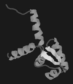
X-ray crystallography [1–7 and references cited therein] is a method to determine the arrangement of atoms within a crystal (Fig. 15.1). In this method, a beam of X-rays strikes a crystal. Then, it scatters into many different directions. The electron density map of the molecule can be generated from the angles and intensities of these scattered beams to build a three-dimensional (3D) picture of the distribution of electrons within the crystal. This leads to the determinations of the mean positions of the atoms in the crystal, as well as their chemical bonds, the disorder, and various other structural properties. A fully grown crystal is mounted on an apparatus called a goniometer. After that, the crystal is gradually rotated and X-rays are passed through it, which produce a diffraction pattern of spots regularly spaced in two dimensions (2D). These are known as reflections. A
3D electron density model of the whole crystal is then created from the images of the crystal that are taken by rotating it at different orientations with the help of Fourier transforms (FT), as well as with previous chemical data for the crystallized sample. Small crystals or deformities in crystal packing lead to erroneous results. X-ray crystallography is related to several other methods for determining atomic structures. Similar diffraction patterns can be produced by scattering electrons or neutrons, which are likewise interpreted as a FT.
The structure of hexamethylenetetramine was solved in 1923, and this happened to be the structure of the first organic molecule. After that, structures of a number of important bioorganic molecules (e.g., porphyrin, corrin, and chlorophyll) were solved.
X-ray crystallography of biological molecules took off with Dorothy Crowfoot Hodgkin, who solved the structures of cholesterol (1937), vitamin B12 (1945), and penicillin (1954). In 1969, she succeeded in solving the structure of insulin.
FIGURE 15.1 An example of a crystal structure. Helices are shown as ribbons and sheets are presented as arrows. The rests are coils.
15.6.1.1 Protein Crystallography.
Crystal structures of proteins, which are irregular, began to be solved in the late 1950s. The first protein structure that was solved by X-ray crystallography was that of sperm whale myoglobin by Max Perutz and Sir John Cowdery Kendrew. Since then, X-ray crystal structures of proteins, nucleic acids, and other biological molecules have been determined. X-ray crystallography has a widespread use in the elucidation of protein structure function relationship, mutational analysis and drug design. The challenge lies in the prediction of structures of membrane proteins (e.g., ion channels and receptors) as it is difficult to find appropriate systems for them to crystallize. The reason is these proteins are integral parts of the cell membranes and it is hard to get the protein part out from the membrane component.
15.6.1.2 Nuclear Magnetic Resonance Methodologies. Proton nuclear magnetic resonance (HNMR) spectroscopy [1–6, 8 and References cited Therein] is a field of structural biology in which NMR spectroscopy is used to obtain information about the structure and dynamics of proteins. Structure determination by NMR spectroscopy usually consists of several phases, each using a separate set of highly specialized techniques. The sample is prepared, resonances are assigned, restraints are generated, and a structure is calculated and validated.
15.6.1.3 Förster Resonance Energy Transfer–Fluorescence Resonance Energy Transfer. Fluorescence resonance energy transfer (FRET) [1–7, 22 and References cited Therein] is a mechanism describing energy transfer between two molecules, both of which should be sensitive to light. This method is used to study protein dynamics, protein–protein, and protein–deoxyribonucleic acid (DNA) interactions. For FRET analysis of protein interactions, the cyan fluorescent protein (CFP)–yellow fluorescent protein (YFP) pair, which is the color variants of the green fluorescent protein (GFP), is currently the most useful protein pair that is being employed in biology. The interactions between the proteins are determined by the amount of energy that is being transferred between the proteins, thereby creating a large emission peak of YFP obtained by the overlaps of the individual fluorescent emission peaks of CFP and YPF as the two proteins are near to each other.
15.6.1.4 Yeast Two-Hybrid System. One of the important methods to analyze the physical interactions between proteins or proteins with DNA is the yeast two-hybrid screening [1–6, 23–26]. The basic principle behind the process stems from the fact that the close proximity and modularity of the activating and the binding domains of most of the eukaryotic transcription factors lead to the interactions between themselves albeit indirectly. This system often utilizes a genetically engineered strain of yeast that does not possess the biosynthetic machinery required for the biosynthesis of amino acids or nucleic acids. Yeast cells do not survive on the media lacking these nutrients. In order to detect the interactions between the proteins, the transcription factor is divided into two domains called the binding (BD) and the activator domain (AD). Genetically engineered plasmids are made to produce a protein product with the DNA binding domain attached onto a protein. Another such plasmid codes for a protein product having the AD tagged to another protein. The protein fused to the BD may be referred to as the bait protein and is typically a known protein that is used to identify the new binding partners. The protein fused to the AD may be referred to as the prey protein and can either be a single known protein or a collection of known or unknown proteins. The transcription of the reporter gene(s) occurs if and only if the AD and BD of the transcription factors are connected bringing the AD close to the transcription start site of the reporter gene, which justifies the presence of physical interactions between the bait and the prey proteins. Thus, a fruitful interaction between the proteins fused together determines the phenotypic change of the cell.
15.6.1.5 Affinity Purification. This technique studies PPIs [1–6]. It involves creating a fusion protein with a designed piece, the tag, on the end. The protein of interest with the tag first binds to beads coated with IgG. Then, the tag is broken apart by an enzyme. Finally, a different part of the tag binds reversibly to beads of a different type. After the protein of interest has been washed through two affinity columns, it can be examined for binding partners.
15.6.1.6 Rotein Chips–Protein Microarray. This method is also sometimes referred to as protein binding microarray [1–6]. It provides a multiplex approach to identify PPIs, to identify transcription factor protein–activation, or to identify the targets of biologically active small molecules. On a piece of glass, different protein molecules or DNA-binding sequences of proteins are affixed orderly at different locations forming a microscopic array. A commonly used microarray is obtained by affixing antibodies that bind antigen molecules from cell lysate solutions. These antibodies can easily be spotted with appropriate dyes.
The aforementioned experimental tools are routinely used in laboratories to detect PPIs. However, these methods are not devoid of shortcomings. They are labor- and time-intensive expensive, and often give poor results. Moreover, the PPI data obtained using these techniques include false positives, which necessitates the use of other methods in order to verify the results. All these led to the development of computational methods that are capable of PPI prediction with sufficient accuracies.
15.6.2 Computational PPI Prediction Methodologies
Computational PPI prediction methodologies can be classified broadly as numerical value-based and probabilistic. Both of them involve training over a data set containing protein structural and sequence information [27–75]. Numerical methods use a function of the form F = f (pi, pj ![]() ni, x), where, pi = input data for the residue i under consideration, pj = the corresponding properties of the spatially neighboring residues and j
ni, x), where, pi = input data for the residue i under consideration, pj = the corresponding properties of the spatially neighboring residues and j ![]() nrm i and x = the collection of coefficients to be determined by training. The value of F determines the characteristics of residue i under consideration. It can either be I for interface or N for noninterface. If F is above a certain threshold, i is considered to be in I state otherwise it is in N state.
nrm i and x = the collection of coefficients to be determined by training. The value of F determines the characteristics of residue i under consideration. It can either be I for interface or N for noninterface. If F is above a certain threshold, i is considered to be in I state otherwise it is in N state.
The value-based methods are classified as follows:
Linear Regression. This method [27, 31, 38, 67, 72, and References cited Therein] predicts the values of the unknown variable from a set of known variables. It also tests the relationship among the variables. In the case of PPI prediction methods, solvent accessibilities of the amino acid residues of the proteins are taken as inputs. The different amino acid residues have different solvent accessibility values depending on whether they are exposed or buried. Based on a collection of such values of known proteins, linear regression methods may be used to predict the nature of amino acids in unknown proteins.
Scoring Function. This is a general knowledge-based approach [31, 36, 41, 47, 48, 67, 72, and References cited Therein]. Scoring functions are based on empirical energy functions having contributions from various data. In this approach, information is generated from know protein–protein complexes present in the protein databank (PDB). This approach takes into account various physicochemical parameters of the protein complexes, (e.g., solvation potential, solvent accessibilities, interaction free energies, and entropies). These data are used to generate the scoring functions for the individual atoms of the amino acids constituting the protein complexes. The functions can then be used in case of unknown proteins to predict its mode of binding. The typical form of a scoring function is as follows:
There are several methods available that use these. The significances of the individual terms are listed below:
Utotal = Total energy of the system
Ubond = Bond energy of the molecules under considerations. In this case, the molecules are protein molecules.
Kb = Force constant associated with the bond in question
r = Actual bond distance in the molecule
req = Equilibrium bond distance
Uangle = Energy associated with change in bond angles from their usual values
Kθ = Force constant associated with the bond angle in question
θ= Actual bond angle in the molecule
θeq= Equilibrium bond angle
Udihedral = Energy associated with change in dihedral angles from their usual values.
Ф = dihedral angle
n = multiplicity (which gives the number of minimum points in the function as the torsion angle changes from 0 to 2π)
δ = phase angle
An = force constant.
Unonbonded = Energy associated with various nonbonded interactions (e.g., H- bonding, etc.). It consists of an electrostatic and a Lennard-Jones term.
The q terms are the partial atomic charges εij and σij are the Lennard-Jones well-depth energy and collision-diameter parameters ε0 is the permittivity of free space and rij is the interatomic distance.
Support Vector Machines. Support vector machines (SVM) [17, 27, 30, 44, 54–59, and References cited Therein] is a supervised learning method for classification, function approximation, signal processing, and regression analysis. In this method, the input data are divided into two different sets, normaly, the interface (I) and noninterface (N) states. The SVM will create a separating hyperplane that maximizes the margin between the two different types of data. The basic principle of SVM is to first train it with a set of known data, which would create a classifier. The classifier is then used to predict whether a residue is on a PPI site or not by giving it a score. The SVM training is done by using a training file consisting of feature vectors generated using various information about the PPI complex. The typical information used for this purpose follow: hydrophobicities, accessible surface areas, electrical charges, sequence similarity and sequence conservation scores of amino acids and so on. This information is combined into feature vectors and used as input to train the SVM.
In terms of mathematics, the problem is defined as follows:
where Ci is a class representing +1 or -1 to which the datapoints Xi (which are nothing but some real vectors) belong. The datapoints are used to train a SVM that creates the maximum-margin hyperplane dividing the points based on the class label. Any hyperplane can be written on the basis of the datapoints (Xi) as
where,“.” is the dot product, F = normal vector perpendicular to the hyperplane, ![]() offset of the hyperplane from the origin along the normal vector F, a and F are chosen in such a way as to maximize the distance between the parallel hyperplanes to enhance the chance of separation of the data.
offset of the hyperplane from the origin along the normal vector F, a and F are chosen in such a way as to maximize the distance between the parallel hyperplanes to enhance the chance of separation of the data.
The representations of the hyperplanes can be done using the equations:
The training data are generally linearly separable, which enables us to select the two hyperplanes of the margin in a way that there are no points between them. Then we try to maximize their distance. Geometrically, the distance between the two hyperplanes is ![]() has to be minimized. In order to prevent datapoints falling into the margin, the following constraints are added:
has to be minimized. In order to prevent datapoints falling into the margin, the following constraints are added:
For each i either, F. Xi-a > 1 for Xi of the first class with label +1 and for the second class (having a label of -1) F. Xi-a < 1. Thus, Ci (F.Xi - a) ≤ 1, for all 1 ≤ i ≤ n. Combining everything the optimization problem looks like Minimization of ![]() , when (for any
, when (for any ![]() . In order to simplify, the above mentioned problem is converted to a quadratic one and the problem looks like Minimization of
. In order to simplify, the above mentioned problem is converted to a quadratic one and the problem looks like Minimization of ![]() , when (for any i=1,…,n)
, when (for any i=1,…,n)
Standard quadratic programming techniques can now be used to solve the problem.
The classification rule can be written in its unconstrained dual form. The dual of the SVM can be shown to be the following optimization problem: Maximization of ![]() , when (for any i=1,…,n)
, when (for any i=1,…,n) ![]() .
.
The w terms are a dual representation for the weight vector in terms of the training set:
For simplicity, sometimes the hyperplane is made to pass through the origin of the coordinate system. Such hyperplanes are called unbiased. General hyperplanes that are not passing through the origin are called biased. An unbiased hyperplane can be made by a = 0 in Eq. (15.1). In that case the expression of the dual remains almost the same without the equality.
Another approach of SVM is called transductive support vector machines. This is an extension of the aforementioned process in such a way that it can incorporate structural properties (e.g., structural correlations) of the test data set for which the classification needs to be done. In this case, the support vector machine is fed a test data set with the test examples that are to be classified, in addition to the training set T
A transductive support vector machine is defined as follows: Minimization of ![]() , when (for any
, when (for any ![]() and
and ![]()
Neural Network. The neural network [60, 61, 67, 72, and References cited Therein] is an interconnected group of artificial neurons (in biological perspective, neurons are connectors that transmit information via chemical signaling between cells), which are basically an adaptive system. There are hidden layers whose output is fed into a final output node. Protein information like the solvent accessibilities, free energy of interactions, and so on, are fed into the hidden layers to train them. Next, the trained model can be used to produce the output from a set of unknown data.
Random Forests. Random forests [40, 42, 63–66, 72, and References cited Therein] are a combination of tree predictors. Each of the trees is dependent on the respective values of a random vector that is sampled independently following the same distribution for all the trees in the whole forest. The more the number of trees the less is the error. Due to the law of large numbers there are no overfitting problems.
The steps of the algorithm can be summarized as follows: Let X = Number of samples in the training data set, Y = Total number of features or variables of the training samples, and y = The number of input variables that are to be employed to come to a decision at a node of the decision tree given that, y < Y.
A training set is therefore chosen for the tree to be generated and it is done by picking up the samples X times from the training data set with replacement. The remaining samples are used as a test data set to estimate the error of the tree, on the basis of the type of classes assigned to them by the classifier to be built on the training data set. The decision at each node is determined by randomly picking up y variables at that particular node and the best combination of the variables is preserved.
Random forest has a number of advantages like:
1. The method can tackle a very large number of input variables in the data sets.
2. It gives an idea of the variable importance to determine classification.
3. It gives an unbiased estimate of error.
4. If there are missing values for a particular variable, the random forests can employ a method for estimating missing data to maintain accuracy.
5. The method can give an idea about the interactions between variables.
6. It does not over fit.
The probabilistic methods are employed to find the conditional probability ![]() , where s is either I or N for the range of input data
, where s is either I or N for the range of input data ![]() for a residue under consideration. Interface is predicted if the value of
for a residue under consideration. Interface is predicted if the value of ![]() becomes greater than a threshold value. This method can be categorized as follows:
becomes greater than a threshold value. This method can be categorized as follows:
Naïve Bayesian. Naïve Bayesian [67, 72, and References cited Therein] is a supervised learning method. It takes input data, which are assumed to be independent. Naïve Bayes is a well-known machine learning tool. This classifier assumes no dependencies between the variables to predict the class of the object under study. The mathematical formulation of the method is as follows:
This equation calculates the probability of predicting the class of an object X, the observed data based on some hypothesis H. The parameter P(H|X) is the posterior probability of H on X, P(X) is the prior probability of X, P(H) is the a priori probability of H that X belongs to the class C, and P(X|H) is the posterior probability of X on H. In this case, the training data is used to build the decision rule. Selection of the most probable class is the rule:
The class is therefore given the maximum probability based on the rules created by training with known data. Protein sequence information can be used to generate rules for the classification. The window selects a central target residue and uses the neighboring residue information to train and predict the residues involved in interactions.
Bayesian Network. In this case [45, 67, 69, 70, 72, and References cited Therein], the input data are dependent on each other. So a joint probability is calculated. For two dependent input data, x1 and x2, their joint probability P(S|x1,x2) is calculated as P(x1, x2|S).
P(S) = fraction of state S in the training dataset. In case of PPIs S represents whether an amino acid residue of the protein under study is in the interface or not.
P(xi) = probability density of input data xi in the whole data set.
P(xi|S) = probability density of input data in the subset with a given state S.
Hidden Markov Model. Hidden Markov models (HMMs) [46, 67, 71, 72, and References cited Therein] are directed graphical models that define a factored probability distribution of p(x,y). The mathematical formulation of the model is
This is often referred to as a generative model. The term p(xi|yi) can be considered to be the probability that the observed result xi is generated from the feature yi. The second term, p(yi|yi - 1), is actually the first-order Markov assumption term. It represents the probability of a label variable yi that is not related to the other label variables yi - 1 used in the study.
In case of prediction of PPIs, this method takes into account a multiple sequence alignment (MSA) of known proteins. The amino acid residues that are found to be conserved in the MSA are used to construct a profile that is used to predict the nature of the amino acids from the protein of interest.
Conditional Random Field. Conditional random field [67, 71–73, and References cited Therein] is a comparatively new method for the prediction of PPIs. In this method, each position along the protein chain is assigned to either a I or N label depending on some feature functions. This method is quite similar to HMM, but as opposed to HMM during prediction, the conditional probability of p(x|y) is calculated.
From a biological point of view, the PPI predictive methodologies may be categorized in somewhat different ways.
Evaluation Based on Whole Genome Analysis. It has been observed that protein- coding genes that are in close proximities in different genomes are known to be interacting with each other [24–26, 67, 72, 74]. Sometimes two proteins fuse together to form a new protein in another organism. They are also considered to be interacting partners. Though the method seems interesting, but in reality it fails to predict interactions between proteins encoded by genes located far in the genome. This approach is not suitable for eukaryotes.
FIGURE 15.2 Prediction of PPIs based on the whole genome analysis.
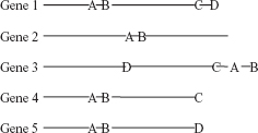
In Figure 15.2, the genes produce proteins A, B, C, and D. Since the distance between the proteins A and B is very small in all the genes, they may be considered to be interacting.
Evaluation Based on Evolutionary Relationships. This method is based on the phylogenetic profiles of the proteins under observations [47, 67, 72, 74, and References cited Therein]. Proteins with similar profiles exhibit functional relationships. Incorporation of evolutionary relationships furthers the prediction method.
TABLE 15.1 Prediction of PPIs Based on Evolutionary Relationships
The genome in Table 15.1 codes for Genes 1–5 with proteins A to E. Proteins A, B, and E share the same phylogenetic profiles. Therefore we may conclude that A, B, and E are interacting among themselves.
Evaluation Based on Protein 3D Structures. This method relies on the solved 3D structures of proteins [17, 31, 33, 37, 40, 47, 67, 72, 74, and References cited Therein]. Proteins having experimentally determined 3D structures can be compared with other such structures for possible sequence identities. A suitable close homologous structure of a protein complex may indicate the possible binding modes of the former with its partner. In general, interface residues are known to be more or less conserved. Therefore, all possible protein pairs between those under observations can be predicted. In other words, the structures of the interacting protein partners are analyzed to find the best possible mode of binding and they are then compared to the existing protein complexes. The possible structures are ranked based on their energy content or some other statistical parameters. This method can also be used to find the putative binding partner from a set of 3D structures of interest.
Evaluation Based on Protein Domains. This method relies on the presence of similar domains in proteins [17, 31, 33, 37, 40, 46, 47, 67, 71, 72, and References cited Therein]. A database of protein families based on protein domains, Pfam, gives an idea about the domain structures in proteins. If the proteins of interest have similar arrangements of domains as those of some other interacting protein pairs, then these former proteins are also considered to have a similar kind interaction pattern as the latter.
Evaluation Based on Primary Structure of Proteins. This method is based on the assumption that PPIs are mediated through a specific number of short sequence motifs [61, 64, 69, 70, 72, 74, and References cited Therein]. Protein sequence information like a position specific scoring matrix (PSSM), combined with other experimental evidences (known interactions, physicochemical properties of amino acids, and so on) can be used as descriptors to train some machine-learning programs (support vector machines, random forest, etc.). The result would predict the probabilities of interactions between protein pairs.
The different methods are applied for different types of input data sets. The combinations of results for the different predictive methodologies may be used to have a comprehensive result. Protein–protein binding modes are also used to predict interfaces. The different computational methods are applied to different data sets with varying degrees of success. The results depend on the type of data used. Some methods are suitable for some specific kinds of data sets. The SVM gives fairly good results if the data set is small and balanced, whereas random forest can handle large data sets. Sometimes SVM can overfit the data, but random forest never does. However, there are a number of challenging problems that need be taken into account. They are
PPIs Associated with Large-Scale Conformational Changes. Large-scale conformational changes, (e.g., those involving domain–domain rearrangements) are difficult to analyze in terms of computation. In such cases, it might be possible for the protein-binding residues in their native complex form to get scattered when they are uncomplexed. This may lead to their elimination in the process of clustering.
One Protein, Many Partners. There are a number of proteins that have multiple partners where the interactions are mediated through the different parts of the surface. In such cases, it is possible that the different binding modes are predicted, but they have to be validated by biochemical data to identify which is for which partner protein.
15.7 DISCUSSION AND CONCLUSION
The PPIs are the central players in many of the vital biochemical processes. Cellular metabolism is guided by the PPIs be it a bacterium, an archea, or complex multicellular organisms. This made the prediction of PPIs so vital. Knowledge of PPI is useful in all aspects of biology. Many of the diseases including cancer are results of improper PPIs. Therefore prediction of PPIs has become important targets for therapy. There are different approaches for the predictions and analyses of protein–protein interactions. This chapter has made an attempt to review the different PPI prediction methodologies that are available. The experimental approaches are more accurate and would give more comprehensive and reliable results; but they are time consuming and labor intensive besides being expensive. As alternatives to the experimental approaches, computational methods have been developed. They are comparatively less accurate, but often give an overall idea of the whole process. There are various computational approaches with somewhat varying accuracies. The most important aspect is that computational approaches are cost effective, and requires less time. A word of caution is that none of the methods are cent percent accurate. To properly predict a PPI, much information is needed. The best way to perform an experiment is first to use the computational algorithms to find a PPI, and then test that via experimental means.
APPENDIX I
This appendix refers to the web links of some of the important servers used in the study of protein–protein interaction. This is not an exhaustive list and the list keeps on growing day by day. This is given for an easy reference of the computational tools available to study protein interactions.
http://protein3d.ncifcrf.gov/∼keskino
http://dockground.bioinformatics.ku.edu/
http://www.ces.clemson.edu/compbio/protcom/
http://mips.gsf.de/proj/yeast/CYGD/interaction/
http://dip.doe-mbi.ucla.edu/dip/Main.cgi
http://www.ncbi.nlm.nih.gov/RefSeq/HIVInteractions/
http://www.ihop-net.org/UniPub/iHOP
http://insilico.csie.ntu.edu.tw:9999/point/
http://point.bioinformatics.tw/
http://www.compbio.dundee.ac.uk/www-pips
http://www.jcvi.org/mpidb/about.php
http://www.molecularconnections.com/home/en/home/products/NetPro
http://www.proteinlounge.com/inter_home.asp
http://itolab.cb.k.u-tokyo.ac.jp/Y2H/
http://mips.gsf.de/genre/proj/mpact/index.html
APPENDIX II
There are a number of techniques that culminate in the generation of numerous software tools for the analysis of PPIs. Of which some of them are mentioned here
PATCHDOCK (http://bioinfo3d.cs.tau.ac.il/PatchDock/). PatchDock algorithm is inspired by object recognition and image segmentation techniques used in Computer Vision. Docking can be compared to assembling a jigsaw puzzle. When solving the puzzle two pieces are matched by picking one piece and searching for the complementary one.
ELM server (http://elm.eu.org/about.html). It is based on the recognition of short linear sequence motifs on proteins (SLiM), which are considered to be the binding regions.
ISEARCH [75]. This method uses known domain–domain interfaces stored in an interface library to screen unbound proteins for structurally similar interaction sites.
GRAMM (http://vakser.bioinformatics.ku.edu/resources/gramm/grammx/). GRAMM is a program for protein docking. To predict the structure of a complex, it requires only the atomic coordinates of the two molecules (no information about the binding sites is needed). The program performs an exhaustive six-dimensional search through the relative translations and rotations of the molecules.
GWIDD (http://gwidd.bioinformatics.ku.edu/). GWIDD is a comprehensive resource for genomewide structural modeling of protein–protein interactions. It contains interaction information for multiple organisms.
The structures of the participating proteins are modeled or crystallographic coordinates are retrieved, if available, and docked by GRAMM-X. The resource is not restricted to interactions in the GWIDD database. Other sequences or structures may be entered at various stages.
Dockground (http://dockground.bioinformatics.ku.edu/). Integrated system of databases for protein recognition studies. The core Dockground data set consists of cocrystallized protein–protein structures. The data set is regularly updated and annotated.
I-2-I Site engine (http://bioinfo3d.cs.tau.ac.il/I2I-SiteEngine).
Interface-to-Interface (I2I)-SiteEngine, is based on the structural alignment between two protein–protein interfaces. The method simultaneously aligns two pairs of binding sites that constitute an interface. The method is based on recognition of similarity of physico-chemical properties and shapes. It assumes no similarity of sequences or folds of the proteins that comprise the interfaces.
INTERVIEWER (http://interviewer.inha.ac.kr/). Protein–protein interaction networks often consist of thousands of nodes or more, which severely limit the usefulness of many graph drawing tools because they become too slow for interactive analysis of the networks and because they produce cluttered drawings with many edge crossings. Interviewer is based on a layout algorithm for visualizing large-scale protein interaction networks.
InterViewer3 (1) first finds a layout of connected components of an entire network, (2) finds a global layout of nodes with respect to pivot nodes within a connected component, and (3) refines the local layout of each connected component by first relocating midnodes with respect to their cutvertices and direct neighbors of the cutvertices and then by relocating all nodes with respect to their neighbors within distance 2.
APID (http://bioinfow.dep.usal.es/apid/index.htm). APID is an interactive bioinformatic webtool that has been developed to allow exploration and analysis of main currently known information about PPIs integrated and unified in a common and comparative platform.
INTEGRATOR (http://bioverse.compbio.washington.edu/integrator/).
Integrator is a tool for graphically searching PPI networks across several genomes. The database contains experimentally determined PPIs from various public repositories (including the DIP, GRID, and PDB) and predicts PPIs based on these collections.
PIPSA (http://projects.villa-bosch.de/mcmsoft/pipsa/3.0/index.html). PIPSA may be used to compute and analyze the pairwise similarity of 3D interaction property fields for a set of proteins. con-PPISP (http://pipe.scs.fsu.edu/ppisp.html). It uses PSI BLAST sequence profile and solvent accessibility as input to a neural network.
PROMATE (http://bioportal.weizmann.ac.il/promate). It is based on a Naïve Bayesian method, which takes secondary structure, amino acid grouping, sequence conservation, and atom distribution as input.
PINUP (http://sparks.informatics.iupui.edu?PINUP/). It is based on an empirical scoring function that involves side chain energy terms, solvent accessible area, and sequence conservation.
PPI-Pred (http://bioinformatics.leeds.ac.uk/ppi-pred). It is based on SVM that considers six parameters.
SPPIDER (http://sppider.cchmc.org/). A neural network based technique. It takes solvent accessibilities as inputs.
SHARP2 (http://www.bioinformatics.sussex.ac.uk/SHARP2). It calculates solvation potential, hydrophobicity, accessible surface area, residue interface propensity, and planarity and protrusion. Each parameter is combined for each surface patch and the patch with the highest value is given as the output.
This is not an exhaustive list. The list is growing day by day.
REFERENCES
1. T. E. Creighton (1996), Proteins: Structures and Molecular Properties, 2nd ed., W. H. Freeman, NY.
2. J. Kyte (1995), Structure in Protein Chemistry, 2nd ed., Garland Publishing Inc., NY.
3. C. Branden and J. Tooze (1999), Introduction to Protein Structure, 2nd ed., Garland Publishing Inc., NY.
4. G. A. Petsko and Dagmar Ringe (2003), Protein Structure and Function (Primers in Biology), 1st ed., New Science Press Ltd., London.
5. D. Voet and J. G. Voet (1995), Biochemistry, 2nd ed., John Wiley & Sons, Inc., NY.
6. A. Fresht (1998), Structure and Mechanism in Protein Science: A Guide to Enzyme Catalysis and Protein Folding, 1st ed., W. H. Freeman, NY.
7. J. Drenth (1994), Principles of protein x-ray crystallography, 2nd ed., Springer, NY.
8. J. Cavanagh, W. J. Fairbrother, A. G. Palmer, III, N. J. Skelton, M. Rance (2006), Protein NMR Spectroscopy: Principles and Practice, 2nd ed., Academic Press, NY.
9. S. Jones and J. M. Thornton (1977), Analysis of protein–protein interaction sites using surface patches, J. Mol. Biol., 272(1), 121–132.
10. S. Jones and J. M. Thornton (1997), Prediction of protein–protein interaction sites using patch analysis, J. Mol. Biol., 272(1), 133–143.
11. Y. Ofran and Burkhard Rost (2003), Analysing six types of protein–protein interfaces, J. Mol. Biol., 325(2), 377–387.
12. A. A. Bogan, and K. S. Thorn (1998), Anatomy of hot spots in protein interfaces, J. Mol. Biol., 280(1), 1–9.
13. Y. Ofran and B. Rost (2007), ISIS: interaction sites identified from sequence, Bioinformatics, 23(20), e13–e16.
14. Y. Ofran and B. Rost (2003), Predicted protein–protein interaction sites from local sequence information, FEBS Lett., 544(1), 236–239.
15. B. Ma, T. Elkayam, H. Wolfson, and R. Nussinov (2003), Protein–protein interactions: Structurally conserved residues distinguish between binding sites and exposed protein surfaces, Proc. Natl. Acad. Sci. USA, 100(10), 5772–5777.
16. Y. Ofran and B. Rost (2007), Protein–protein interaction hotspots carved into sequences, PLoS Compu. Biol., 3(7), e119.
17. Jo-Lan Chung, W. Wang, and P. E. Bourne (2006), Exploiting sequence and structure homologs to identify protein–protein binding sites, Proteins: Struct. Function Bioinformatics, 62(3), 630–640.
18. D. Reichmann, O. Rahat, S. Albeck, R. Meged, O. Dym, and G. Schreiber (2005), The modular architecture of protein-protein binding interfaces, Proc. Natl. Acad. Sci. USA, 102(1), 57–62.
19. O. Keskin, B. Ma, and R. Nussinov (2005), Hot regions in protein–protein interactions: The organization and contribution of structurally conserved hot spot residues, J. Mol. Biol., 345(5), 1281–1294.
20. S. Jones and J. M. Thornton (1996), Principles of protein–protein interactions, Proc. Natl. Acad. Sci. USA, 93(1), 13–20.
21. W. L. DeLano (2002), Unraveling hot spots in binding interfaces: progress and challenges, Curr. Opin. Struct. Biol., 12(1), 14–20.
22. A. A. Deniz, T. A. Laurence, G. S. Beligere, M. Dahan, A. B. Martin, D. S. Chemla, P. E. Dawson, P. G. Schultz, S. Weiss (2000), Single-molecule protein folding: Diffusion fluorescence resonance energy transfer studies of the denaturation of chymotrypsin inhibitor 2, Proc. Natl. Acad. Sci. USA, 97(10), 5179–5184.
23. J. A. Wells (1991), Systematic mutational analyses of protein–protein interfaces, Methods Enzymol., 202, 390–411.
24. P. Uetz et al. (2000), A comprehensive analysis of protein–protein interactions in Saccharomyces cerevisiae, Nature (London), 403(6770), 623–627.
25. Y. Ho et al. (2002), Systematic identification of protein complexes in Saccharomyces cerevisiae by mass spectrometry, Nature (London), 415(6868), 180–183.
26. J. Wang et al. (2009), Uncovering the rules for protein-protein interactions from yeast genomic data, Proc. Natl. Acad. Sci.,106(10), 3752–3757.
27. I. Ezkurdia et al. (2009), Progress and challenges in predicting protein-protein interaction sites, Briefings Bioinforamtics, 10(3), 233–246.
28. K. L. Morrison and G. A. Weiss (2001), Combinatorial alanine-scanning, Curr. Opin. Chem. Biol., 5(3), 302–307.
29. A. A. Bogan and K. S. Thorn (2001), ASEdb: a database of alanine mutations and their effects on the free energy of binding in protein interactions, Bioinformatics, 17(3), 284–287.
30. A. Koike and T. Takagi (2004), Prediction of protein–protein interaction sites using support vector machines, Protein Eng. Des. Sel. 17(2), 165–173.
31. H. Neuvirth, R. Raz, and G. Schreiber (2004), ProMate: A Structure Based Prediction Program to Identify the Location of Protein–Protein Binding Sites, J. Mol. Biol., 338(1), 181–199.
32. F. Pazos and A. Valencia (2002), In silico two-hybrid system for the selection of physically interacting protein pairs, Proteins: Struct., Function Bioinformatics, 47(2), 219–227.
33. I. Re, I. Mihalek, and O. Lichtarge (2005), An evolution based classifier for prediction of protein interfaces without using protein structures, Bioinformatics, 21(10), 2496–2501.
34. N. Zaki et al. (2009), Protein–protein interaction based on pairwise similarity, BMC Bioinformatics, 10(150), 150–162.
35. B. Wang et al. (2005), Predicting protein interaction sites from residue spatial sequence profile and evolution rate, FEBS Lett., 580, 380–384.
36. J. Fernández-Recio, M. Totrov, and R. Abagyan, Identification of Protein–Protein Interaction Sites from Docking Energy Landscapes, J. Mol. Biol., 335(3), 843–865.
37. A. Garg, H. Kaur, and G.P. Raghava (2005), Real value prediction of solvent accessibility in proteins using multiple sequence alignment and secondary structure, Proteins, 61(2), 318–324.
38. M. Wagner, R. Adamczak, A. Porollo, and J. Meller (2005), Linear regression models for solvent accessibility prediction in proteins, J Comput. Biol., 12(3), 355–369.
39. Z. Yuan and B. Huang (2004), Prediction of protein accessible surface areas by support vector regression, Proteins, 57(3), 558–564.
40. M. Šikić, S. Tomić, and K. Vlahoviček, Prediction of Protein–Protein Interaction Sites in Sequences and 3D Structures by Random Forests, PLoS Comput. Biol., 5(1).
41. S. J Wodak and R. Méndez (2004), Prediction of protein–protein interactions: the CAPRI experiment, its evaluation and implications, Curr. Opin. Struct. Biol., 14(2), 242–249.
42. X-W. Chen and M. Liu (2005), Prediction of protein–protein interactions using random decision forest framework, Bioinformatics, 21(24), 4394–4400.
43. L. Banci, I. Bertini, V. Calderone, N. Della-Malva, I. C. Felli, S. Neri, A. Pavelkova, and A. Rosato (2009), Copper(I)-mediated protein–protein interactions result from suboptimal interaction surfaces, Biochem. J., 10, 37–42.
44. J. R. Bradford and D. R. Westhead, Improved prediction of protein–protein binding sites using a support vector machines approach, Bioinformatics, 21(8), 1487–1494.
45. J. R. Bradford, C. J. Needham, A. J. Bulpitt, and D. R. Westhead (2006), Insights into Protein–Protein Interfaces using a Bayesian Network Prediction Method, J. Mol. Biol., 362(2), 365–387.
46. T. Friedrich, B. Pils, T. Dandekar, J. Schultz, and T. Müller (2006), Modelling interaction sites in protein domains with interaction profile hidden Markov models. Bioinformatics, 22(23), 2851–2857.
47. M. Landau et al., (2005), ConSurf 2005: the projection of evolutionary conservation scores of residues on protein structures, Nucleic Acids Res., 33(Web Server Issue), w299–w302.
48. N. J. Burgoyne and R. M. Jackson (2006), Predicting protein interaction sites: binding hot-spots in protein–protein and protein-ligand interfaces, Bioinformatics, 22(11), 1335–1342.
49. A. Koike and T. Takagi (2004), Prediction of protein–protein interaction sites using support vector machines, Protein Eng. Des. Sel., 17(2).
50. C. H. Yan, et al. (2004), Identification of interface residues in protease-inhibitor and antigen-antibody complexes: a support vector machine approach, Neural Comput. Appl., 13, 123–129.
51. D. Meyer, F. Leisch, and K. Hornik (2003), The support vector machine under test, Neurocomputing, 55(1–2), 169–186.
52. C. Cortes and V. Vapnik (1995), Support-Vector Networks, Machine Learning, 20.
53. M. Aizerman, E. Braverman, and L. Rozonoer (1964), Theoretical foundations of the potential function method in pattern recognition learning, Automation Remote Control, 25, 821–837.
54. B. E. Boser, I. M. Guyon, and V. N. Vapnik (1992), A training algorithm for optimal margin classifiers, D. Haussler (ed.), 5th Annual ACM Workshop on COLT, ACM Press, Pittsburgh, PA, pp. 144–152
55. H. Drucker, C. J. C. Burges, L. Kaufman, A. Smola, and V. Vapnik (1996), Support Vector Regression Machines. Advances in Neural Information Processing Systems 9 NIPS MIT Press, MA pp. 155–161.
56. M. Ferris and T. Munson (2002), Interior-point methods for massive support vector machines, SIAM J. Optimization 13, 783–804.
57. V. Vapnik (1995), The Nature of Statistical Learning Theory, Springer-Verlag, NY.
58. V. Vapnik and S. Kotz (2006), Estimation of Dependences Based on Empirical Data. Springer, NY, 291–400.
59. O. Ivanciuc (2007), Applications of Support Vector Machines in Chemistry, Rev. Comput. Chem., 23.
60. H. Chen and H-X Zhou (2005), Prediction of interface residues in protein–protein complexes by a consensus neural network method: test against NMR data, Proteins, 61(1), 21–35.
61. P. Fariselli et al. (2002), Prediction of protein–protein interaction sites in heterocomplexes with neural networks, Eur. J. Biochem., 269(5), 1356–1361.
62. A Porollo and J Meller (2007), Prediction-based fingerprints of protein–protein interactions, Proteins, 66(3), 630–645.
63. Y. Qi, J. Klein-Seetharama, and Z. Bar-Joseph (2005), Random forest similarity for protein-protein interaction prediction from multiple sources, Pac. Symp. Biocomput., 10, 531–542.
64. M. Šikić, S. Tomić, and K. Vlahoviček (2009), Prediction of Protein Protein Interaction Sites in Sequences and 3D Structures by Random Forests, Plos Computa. Biol., W. H. Freeman, NY.
65. L. Breiman (2002), Looking inside the black box, Wald Lecture II. Available at www.stat.berkley.edu/-brelman/wald 2002–2 pdf.
66. L. Breiman (2001), Random Forests, Machine Learning, 45.
67. L. Skrabanek, H. K Saini, G. D Bader, and A. J Enright (2008), Computational prediction of protein–protein interactions, Mole. Biotechnol. 38(1), 1–17.
68. C. Wang, J. Cheng, S. Su, and D. X (2008), Identification of Interface Residues Involved in Protein–Protein Interactions Using Naïve Bayes Classifier, Lecture Notes in Artificial Intelligence 5139.
69. J. R. Bradford, C. J. Needham, A. J. Bulpitt, and D. R. Westhead (2006), Insights into protein–protein interfaces using a Bayesian network prediction method, J. Mol. Biol., 362 (2).
70. R. Jansen et al. (2003), A Bayesian Networks Approach for Predicting Protein–Protein Interactions from Genomic Data, Science, 302 (5644), 449–453.
71. T. Friedrich et al. (2006), Modelling interaction sites in protein domains with interaction profile hidden Markov models, Bioinformatics, 22 (23), 2851–2852.
72. H.-X. Zhou and S. Qin (2007), Interaction-site prediction for protein complexes: a critical assessment, Bioinformatics, 23(17), 2203–2209.
73. M.-H. Li, L. Lin, X-L. Wang, and T. Liu (2007), Protein–protein interaction site prediction based on conditional random fields, Bioinformatics, 23(5), 597–604.
74. S. Pitre, Md. Alamgir, J. R Green, M. Dumontier, F. Dehne, and A. Golshani (2008), Computational methods for predicting protein–protein interactions, Adv. Biochem. Eng. Biotechnol. 110.
75. S. Günther, P. May, A. Hoppe A, C. Frömmel, and R. Preissner (2007), Docking without docking: ISEARCH–prediction of interactions using known interfaces, Proteins, 69(4), 839–844.