
CHAPTER 9
KERNEL FUNCTION APPLICATIONS IN CHEMINFORMATICS
9.1 INTRODUCTION
The fast accumulation of data describing chemical compound structures and biological activity calls for the development of efficient informatics tools. Cheminformatics is a rapidly emerging research discipline that employs a wide array of statistical, data mining, and machine learning techniques with the goal of establishing robust relationships between chemical structures and their biological properties. Hence, cheminformatics is an important component on the application side of applying informatics approach to life science problems. It has a broad range of applications in chemistry and biology; arguably the most commonly known roles are in the area of drug discovery where cheminformatics tools play a central role in the analysis and interpretation of structure–activity data collected by various means of modern high throughput screening technology. Traditionally, the analysis of large chemical structure–activity databases was done only within pharmaceutical companies, and up until recently the academic community has had only limited access to such databases. This situation, however, has changed dramatically in very recent years.
In 2002, the National Cancer Institute created the Initiative for Chemical Genetics (ICG) with the goal of offering to the academic research community a large database of chemicals with their roles in cancer research [11]. Two years later, the National Health Institute (NIH) launched a Molecular Libraries Initiative (MLI) that included the formation of the national Molecular Library Screening Centers Network (MLSCN). MLSCN is a consortium of 10 high-throughput screening centers for screening large chemical libraries [2]. Collectively, ICG and MLSCN aim to offer to the academic research community the results of testing about a million compounds against hundreds of biological targets. To organize this data and to provide public access to the results, the PubChem and Chembank database have been developed as the central repository for chemical structure–activity data. These databases currently contain >18 million chemical compound records, >1000 bioassay results, and links from chemicals to bioassay description, literature, references, and assay data for each entry.
Many machine learning and data mining algorithms have been applied to study the structure–activity relationship of chemicals. For example, Xue et al. reported promising results of applying five different machine learning algorithms: logistic regression, C4.5 decision tree, k-nearest neighbor, probabilistic neural network, and support vector machines, to predicting the toxicity of chemicals against an organism of Tetrahymena pyriformis [3]. Advanced techniques, [e.g., random forest and MARS (multivariate adaptive regression splines)] have also been applied to cheminformatics applications [4,5].
This chapter, addresses as the problem of graph classification through study of kernel functions and the application of graph classification in chemical quantitative structure–activity relationship (QSAR) study. Graphs, especially the connectivity maps, have been used for modeling chemical structure for decades. In a connectivity map, nodes represent atoms and edges represent chemical bounds between atoms.
Recently, support vector machines (SVM) have gained popularity in drug design and cheminformatics. A key insight of SVM is the utilization of kernel functions (i.e., inner product of two points in a Hilbert space) to transform a nonlinear classification problem into a linear one. Design of a good kernel function for graphs is therefore a critical issue. The initial effort to define kernels for semistructured data was done by Haussler in his work on the R-Convolution kernel, which provided a framework that many current graph kernel functions follow [6].
While kernel functions and classifier (e.g., SVMs) for graphs have received a great deal of attention recently, most approaches are stymied by graph complexity. Precise comparisons are slow to compute, but simpler methods do not capture enough information about graph topology and structure. The focus of this work is to augment simple graph representations with structure information, allowing the use of fast kernel functions while recognizing important topological similarities. This work draws from several studies: incorporating structure feature graphs into kernel functions [7], extensions for approximate matching of such structure features [8], set-based matching kernels with structure features [9], and an application of wavelets for simplified topology comparison in graph kernels [10].
The material presented here explores some graph kernel functions that improve on existing methods with respect to both classification accuracy and kernel computation time. The following key insights are explored. First, problem relevant structure features can be used to annotate graph vertices in an alignment-based kernel function, raising model accuracy and adding explanatory capability [7]. Second, extensions for matching approximate structure features [8], as well as a faster, simpler kernel function [9], lead to gains in accuracy, as well as faster computation time. Finally, wavelet functions can be applied to graphs in order to summarize feature information in local graph topology, greatly reducing the kernel computation time [10]. We demonstrate a comprehensive experimental study, in the context of QSAR study in cheminformatics, for graph-based modeling and classification.
9.2 BACKGROUND
Before proceeding to algorithmic details, this chapter presents some general background material from a variety of directions. The work of this chapter draws from techniques in data mining, as well as machine learning and chemical property prediction. This chapter will address the following topics: chemical structures as graphs, graph classification, kernel functions, graph mining, and wavelet analysis for graphs.
9.2.1 Chemical Structure
Chemical compounds are organic molecules that are easily modeled by a graph representation. In this approach, nodes in a graph model atoms in a chemical structure and edges in the graph to model chemical bonds in the chemical structure. In this representation, nodes are labeled with the atom element type, and edges are labeled with the bond type (single, double, and aromatic bond). The edges in the graph are undirected, since there is no directionality associated with chemical bonds. Figures 9.1 shows an example chemical structure, where unlabeled vertices are assumed to be carbon (C).
Figures 9.2 shows two sample chemical structures on the left, and their graph representation on the right.
FIGURE 9.1 An example chemical structure.
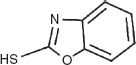
FIGURE 9.2 Graph representations of chemicals.

9.2.2 Graph Classification
Many classifiers exist for classification of objects as feature vectors. The feature vector embeds objects as points in a space where the data is modeled. Recently, an important linear classifier has gained a great deal of attention, the SVM. It is not only fast to train with great model generalization power, but it is also a kernel classifier giving it additional advantages over established vector space classifiers. These issues will be addressed in Section 9.2.3 on kernel functions.
The SVM builds a classification model by finding a linear hyperplane that best separates the classes of data objects. The optimal separating hyperplane (OSH) is chosen by maximizing the margin between the hyperplane and the nearest data points (termed support vectors).
When data are not linearly separable, called the soft-margin case, the SVM finds a hyperplane that optimizes an additional constraint. Often this constraint is a penalty for misclassified samples expressed in various ways.
The problem of finding an OSH is formulated as a convex optimization problem. Hence, it can leverage very powerful algorithms for exactly finding the OSH. Once a OSH has been found, classification of additional objects is easily determined by finding which side of the hyperplane the object resides on. The efficiency of these operations makes SVM an extremely fast classifier. Since the SVM model ideally depends only on a small number of support vectors, it generalizes well and is compact to store.
Crucially, the SVM problem can be formulated such that it represents objects using only the dot products between their vectors. This modification allows the dot products to be replaced with a kernel function between objects, the use of which is discussed further in Section 9.2.3.
9.2.3 Kernel Functions
A kernel function K is a mapping between a pair of graphs into a real number, ![]() . This function defines an inner product between two graphs and must satisfy the following properties:
. This function defines an inner product between two graphs and must satisfy the following properties:
Such a function embeds graphs or any other objects into a Hilbert space, and is termed a Mercer kernel from Mercer’s theorem.
Kernel functions can enhance classification in two ways: first, by mapping vector objects into higher dimensional spaces; second, by embedding nonvector objects in an implicitly defined space. The advantages of mapping objects into a higher dimensional space, the so-called kernel trick, are apparent in a variety of cases where objects are not separable by a linear decision boundary.
This implicit embedding is not only useful for nonlinear mappings, but also serves to decouple the object representation from the spatial embedding. A kernel function need only be defined between data objects in order to apply SVM classification. Therefore SVM can be used for classification of graph objects by defining a kernel function between graphs, without explicitly defining any set of graph features.
9.2.4 Graph Database Mining
This section discusses a few important definitions for graph database mining: labeled graphs, subgraph isomorphic relation, and graph classification.
Definition 9.2.1 A labeled graph G is a quadruple G = (V, E, Σ, λ ) where V is a set of vertices or nodes and E ⊆ V × V is a set of undirected edges. A set of (disjoint) vertex and edge labels Σ, and λ: V ∪ E → Σ is a function that assigns labels to vertices and edges. Assume that a total ordering is defined on the labels in Σ.
A graph database is a set of labeled graphs.
Definition 9.2.2 A graph G′ = (V′,E′, Σ′, λ′) is subgraph isomorphic to G = (V,E, Σ, λ), denoted by G′ ⊆ G, if there exists a 1-1 mapping f: V′ → V such that
The function f is a subgraph isomorphism from graph G′ to graph G. It is said G′ occurs in G if G′ ⊆ G. Given a subgraph isomorphism f, the image of the domain V′ (f(V′)) is an embedding of G′ in G.
Example 9.1 Figures 9.3 shows a graph database of three labeled graphs. The mapping (isomorphism) q1 → p3, q2 → p1, and q3 → p2 demonstrates that graph Q is subgraph isomorphic to P, and hence Q occurs in P. Set p1, p2, p3 is an embedding of Q in P. Similarly, graph S occurs in graph P, but not Q.
FIGURE 9.3 A database of three labeled graphs.

Problem Statement: Given a graph space G∗, a set of n graphs sampled from G∗ and the related target values of these graphs ![]() the graph classification problem is to estimate a function F: G∗ → T that accurately map graphs to their target value.
the graph classification problem is to estimate a function F: G∗ → T that accurately map graphs to their target value.
By classification, all target values are assumed to be discrete values, otherwise it is a regression problem. Below, several algorithms are reviewed for graph classification that work within a common framework called a kernel function. The term kernel function refers to an operation of computing the inner product between two points in a Hilbert space. Kernel functions are widely used in classification of data in a high-dimensional feature space.
9.2.5 Wavelet Analysis for Graphs
Wavelet functions are commonly used as a means for decomposing and representing a function or signal as its constituent parts, across various resolutions or scales. Wavelets are usually applied to numerically valued data (e.g., communication signals or mathematical functions), as well as to some regularly structured numeric data (e.g., matrices and images).
Graphs, however, are arbitrarily structured and may represent many relationships and topologies between data elements. Recent work has established the successful application of wavelet functions to graphs for multiresolution analysis [11]. The use of wavelets in this capacity is different than the use of wavelets for signal and image compression (e.g., in [12]). The complex graph topology must be projected into a Euclidean space, and wavelets are used to summarize the information in the local topology around graph nodes.
Given a vertex v in graph G, define the h-hop neighbors of v as the set of other nodes in G whose shortest path to v is h nodes. The sets of h-hop neighbors then lead to the notion of hop distance, which suitably projects the nodes of a graph into Euclidean space.
Wavelets are then used to summarize feature information in the local topology around vertices in a graph. Since regions near the origin in a wavelet function are strongly positive, while the regions farther away are strongly negative, the distant regions are neutral. By using a wavelet function to compute a weighted sum over vertex features arranged according to hop distance corresponds to a comparison of vertex features in the local neighborhood to those in the distant neighborhood.
9.3 RELATED WORKS
Given that graphs are such powerful and interesting structures, their classification has been extensively studied. This chapter reviews the related work covering pattern mining, kernel functions, and wavelets for graph analysis.
This section surveys work related to graph classification methods by dividing them into two categories. The first category explicitly collects a set of features from the graphs. The possible features included are both structural and chemical. Structural features are graph fragments of different types. Examples are paths, cycles, trees, and general subgraphs [13]. Chemical descriptors, as they are called in QSAR work, are properties describing a molecule overall (e.g., as weight and charge).
Once a set of features is determined, a graph is described by a feature vector, and any existing classification methods (e.g., CBA [14] and decision tree [15]) that work in an n-dimensional Euclidian space, may be applied for graph classification.
The second classification approach is to implicitly collect a (possibly infinite) set of features from graphs. Rather than computing the features, this approach computes the similarity of graphs, using the framework of kernel functions [16]. The advantage of a kernel method is that it has a lower chance of over fitting, which is a serious concern in high-dimensional space with low sample size.
The following sections summarize recent work related to pattern mining and structural features, as well as vector-based classification, kernel functions for classification, and wavelets for graphs.
9.3.1 Pattern Mining
Algorithms that search for frequent patterns (e.g., trees, paths, and cyclic graphs) in graphs can be roughly divided into three groups.
The first group uses a level-wise search strategy, including AGM [17] and FSG [18]. The second category takes a depth-first search strategy, including gSpan[19] and FFSM [20]. Different from level-wise search algorithms AGM and FSG, the depth-first search strategy utilizes a back-track algorithm to mine frequent subgraphs. The advantage of a depth-first search is a better memory utilization, since depth-first search keeps one frequent subgraph in memory and enumerates its supergraphs, in contrast to keeping all k-edge frequent subgraph in memory.
The third category of frequent subgraph mining algorithms does not work directly on a graph space to identify frequent patterns. Instead, algorithms in this category first project a graph space to another space (e.g., that of trees), then identify frequent patterns in the projected space, and finally reconstruct all frequent patterns in the graph space. This strategy is called progressive mining. Algorithms in this category includes SPIN [21] and GASTON [22].
9.3.1.1 Frequent Subgraphs Frequent subgraph mining is a technique used to enumerate graph substructures that occur in a graph database with at least some specified frequency. This minimum frequency threshold is termed the support threshold by the data mining community. After limiting returned subgraphs by frequency, types found can be further constrained by setting upper and lower limits on the number of vertices they can contain. In much of this articles work, the FFSM algorithm [23] is used for fast computation of frequent subgraphs. Figures 9.4, shows an example of this frequent subgraph enumeration. Some work has been done by Deshpande et al. [24] toward the use of these frequent substructures in the classification of chemical compounds with promising results.
FIGURE 9.4 Example graphs and frequent subgraphs (support = 2/3).

9.3.1.2 Chemical Properties and Target Prediction A target property of the chemical compound is a measurable quantity of the compound. There are two categories of target properties: continuous (e.g., binding affinities to a protein) and discrete target properties (e.g., active compounds vs inactive compounds).
The relationship between a chemical compound and its target property is typically investigated through a quantitative structure–property relationship (QSPR). (Such a study a also known as a quantitative structure–activity relationship (QSAR), but property refers to a broader range of applications than activity.) Abstractly, any QSPR method generally may be defined as a function that maps a chemical space to a property space in the form of
Here, D is a chemical structure, P is a property, and the function ![]() is an estimated mapping from a chemical to a property space.
is an estimated mapping from a chemical to a property space.
Different QSPR methodologies can be understood in terms of the types of target property values (continuous or discrete), types of features, and algorithms that map descriptors to target properties.
9.3.2 Vector-Based Classification
Several classification algorithms based on explicitly collected features exist for graph classification in a variety of applications. What follows is a brief survey of popular methods for some pertinent applications
Recent methods applied to QSAR and chemical activity prediction include decision trees, classification based on association [14], and random forest among many others. Decision trees use a collection of simple learners organized in a hierarchical tree structure to classify a object. Nonleaf nodes make decisions about an object based on one of it’s properties and send it to one of the children. Leaf nodes of the tree correspond to classification categories. Random forest uses a collection of randomly generated decision trees and typically classify an object according to the mode of the classes returned by all trees.
Classification based on association (CBA) is somewhat different than these other methods. It seeks to find a set of association rules of the form A → ci, where A is some set of properties and ci is a class label. The XRules [13] are similar to CBA and utilize frequent tree patterns to build a rule-based classifier for XML data. Specifically, XRules first identifies a set of frequent tree patterns. An association rule: G → ci is then formed where G is a tree pattern and ci is a class label. The confidence of the rule is the conditional probability ![]() estimated from the training data. The XRules carefully selects a subset of rules with high confidence values and uses those rules for classification.
estimated from the training data. The XRules carefully selects a subset of rules with high confidence values and uses those rules for classification.
Graph boosting [25] also utilizes substructures toward graph classification. Similar to XRules, graph boosting uses rules with the format of G → ci. Different from XRules, it uses the boosting technique to assign weights to different rules. The final classification result is computed as the weighted majority.
9.3.3 Kernel Functions for Graph Classification
The term kernel function refers to an operation for computing the inner product between two vectors in a feature space, thus avoiding the explicit computation of coordinates in that feature space. Graph kernel functions are simply kernel functions that have been defined to compute the similarity between two graph structures. In recent years, a variety of graph kernel functions have been developed, with promising results as described by Ralaivola et al. [26].
Graph kernel functions can be roughly divided into two categories. The first group of kernel functions consider the full adjacency matrix of graphs, and hence measured the global similarity of two graphs. These include product graph kernels [27], random walk based kernels [28], and kernels based on the shortest paths between a pair of nodes [29]. The second group of kernel functions tries to capture the local similarity of two graphs by counting the shared subcomponents of graphs. These include the subtree [30], cyclic [31], and spectrum kernels [24]. This section reviews the relevant work on these kernel functions.
Product graph kernels use a feature space of all possible node label sequences for walks in graphs. Since the number of possible walks are infinite, there is no way to enumerate all the features in kernel computation [27]. Instead, a product graph is computed in order to make the kernel function computation feasible.
Rather than computing the shared paths exactly, which has prohibitive computational cost for large graphs, the work of Kashima et al. [28] is based on the use of shared random label sequences in the computation of graph kernels. Their marginalized graph kernel uses a Markov model to randomly generate walks of a labeled graph. The random walks are created using a transition probability matrix combined with a walk termination probability. These collections of random walks are then compared and the number of shared sequences is used to determine the overall similarity between two molecules.
Spectrum kernels aim to simplify the aforementioned kernels by working in a finite-dimensional feature space based on a set of subgraphs (or as special cases, trees, cycles, and paths). The kernel function is computed as the inner product between two feature vectors (e.g., counts of subgraph occurrences) as in [24]. Transformations of the inner product (e.g., minmax kernel [32] and Tanimoto kernel [26], are also widely used. The subtree kernel [33] is a variation on the spectrum kernel that uses subtrees instead of paths.
The optimal assignment kernel, described by Frölich et al. [10], differs significantly from the marginalized graph kernel. This kernel function first computes the similarity between all vertices in one graph and all vertices in another. The similarity between the two graphs is then computed by finding the maximal weighted bipartite graph between the two sets of vertices, called the optimal assignment. The authors investigate an extension of this method whereby certain structure patterns defined a priori by expert knowledge, are collapsed into single vertices, and this reduced graph is used as input to the optimal assignment kernel.
9.3.4 Wavelets Functions for Graphs
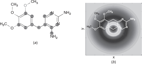
Crovella and Kolaczyk [11] developed a multiscale method for network traffic data analysis. For this application, they are attempting to determine the scale at which certain traffic phenomena occur. They represent traffic networks as graphs labeled with some measurement (e.g., bytes carried per unit time). In their method, they use the hop distance between vertices in a graph, defined as the length of the shortest path between them, and apply a weighted average function to compute the difference between the average of measurements close to a vertex and measurements that are far, up to a certain distance. This process produces a new measurement for a specific vertex that captures and condenses information about the vertex neighborhood. Figures 9.5 shows a diagram of wavelet function weights overlayed on a chemical structure.
FIGURE 9.5 A chemical graph and hop distances. From [10], with permission.
Maggioni et al. [12] demonstrate a general purpose biorthogonal wavelet for graph analysis. In their method, they use the dyadic powers of an diffusion operator to induce a multiresolution analysis. While their method applies to a large class of spaces, (e.g., manifolds and graphs), the applicability of their method to attributed chemical structures is not clear. The major technical difficulty is how to incorporate node labels in a multiresolution analysis.
9.4 ALIGNMENT KERNELS WITH PATTERN-BASED FEATURES
Traditional approaches to graph similarity rely on the comparison of compounds using a variety of molecular attributes known a priori to be involved in the activity of interest. Such methods are problem-specific, however, and provide little assistance when the relevant descriptors are not known in advance. Additionally, these methods lack the ability to provide explanatory information regarding what structural features contribute to the observed chemical activity. The method proposed here, referred to as OAPD for Optimal-Assignment with Pattern-Based Descriptors, alleviates both of these issues through the mining and analysis of structural patterns present in the data in order to identify highly discriminating patterns, which then augment a graph kernel function that computes molecular similarity.
9.4.1 Structure-Based Pattern Mining for Chemical Compound Classification
The following sections outline the algorithm that drives the experimental method. In short, it measures the similarity of graph structures whose vertices and edges have been labeled with various descriptors. These descriptors represent physical and chemical information (e.g., atom and bond types). They are also used to represent the membership of atoms in specific structure patterns that have been mined from the data. To compute the similarity of two graphs, the vertices of one graph are aligned with the vertices of the second graph, such that the total overall similarity is maximized with respect to all possible alignments. Vertex similarity is measured by comparing vertex descriptors, and is computed recursively so that when comparing two vertices, it also compares the neighbors of those vertices, and their neighbors, and so on.
9.4.1.1 Structure Pattern Mining The frequent subgraph mining problem can be phrased as such: Given a set of labeled graphs, the support of an arbitrary subgraph is the fraction of all graphs in the set that contain that subgraph. A subgraph is frequent if its support meets a certain minimum threshold. The goal is to enumerate all the frequent, connected subgraphs in a graph database. The extraction of important subgraph patterns can be controlled by selecting the proper frequency threshold, as well as other parameters (e.g., size and density) of subgraph patterns.
9.4.1.2 Optimal Assignment Kernel The optimal assignment kernel function computes the similarity between two graph structures. This similarity computation is accomplished by first representing the two sets graph vertices as a bipartite graph, and then finding the set of weighted edges assigning every vertex in one graph to a vertex in the other. The edge weights are calculated via a recursive vertex similarity function. This section presents the equations describing this algorithm in detail, as discussed by Frölich et al. 34]. The top-level equation describing the similarity of two molecular graphs is
where (π) denotes a permutation of a subset of graph vertices, and (m) is the number of vertices in the smaller graph. This information is needed to assign all vertices of the smaller graph to vertices in the large graph. The (knei) function, which calculates the similarity between two vertices using their local neighbors, is given as follows:
The functions (kv) and (ke) compute the similarity between vertices (atoms) and edges (bonds), respectively. These functions could take a variety of forms, but in the OA kernel they are RBF functions between vectors of vertex–edge labels.
The (γ(l)) term is a decay parameter that weights the similarity of neighbors according to their distance from the original vertex. The (l) parameter controls the topological distance within which to consider neighbors of vertices. The (Rl) equation, which recursively computes the similarity between two specific vertices, is given by the following equation:
where (|v|) is the number of neighbors of vertex (v), and (nk(v)) is the set of neighbors of (v). The base case for this equation is (R0), defined by
The notation (v → ni(v)) refers to the edge connecting vertex v with the (i)th neighboring vertex. The functions (kv) and (ke) are used to compare vertex and edge descriptors, by counting the total number of descriptor matches.
9.4.1.3 Reduced Graph Representation One way in which to utilize the structure patterns that are mined from the graph data is to collapse the specific subgraphs into single vertices in the original graph. This technique is explored by Frölich et al. [10] with moderate results, although they use predefined structure patterns, so called pharmacophores, identified a priori with the help of expert knowledge. The method proposed here ushers these predefined patterns in favor of the structure patterns generated via frequent subgraph mining.
The use of a reduced graph representation has some advantages. First, by collapsing substructures, an entire set of vertices can be compared at once, reducing the graph complexity and marginally decreasing computation time. Second, by changing the substructure size, the resolution at which graph structures are compared can be adjusted. The disadvantage of a reduced graph representation is that substructures can only be compared directly to other substructures, and cannot align partial structure matches. As utilized in Frölich et al. [34], this is not as much of a burden since they have defined the best patterns a priori using expert knowledge. In the case of the method presented here, however, this is a significant downside, as there is no a priori knowledge to guide pattern generation and we wish to retain as much structural information as possible.
9.4.1.4 Pattern-Based Descriptors The loss of partial substructure alignment following the use of a reduced graph representation motivated us to find another way of integrating this pattern-based information. Instead of collapsing graph substructures, vertices are simply annotated with additional descriptor labels indicating the vertex’s membership in the structure patterns that were previously mined. These pattern-based descriptors are calculated for each vertex and are used by the optimal assignment kernel in the same way that other vertex descriptors are handled. In this way, substructure information can be captured in the graph vertices without needing to alter the original graph structure.
9.4.2 Experimental Study
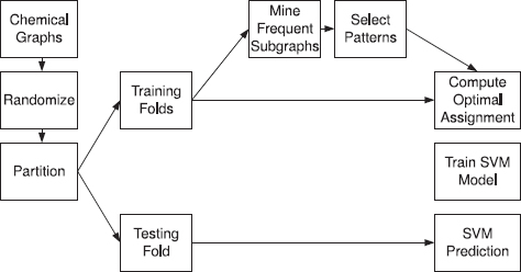
Classification experiments were conducted on five different biological activity data sets, and measured SVM classifier prediction accuracy for several different feature generation methods. The data sets and classification methods are described in more detail in the following sections, along with the associated results. Figure 9.6 gives a graphical overview of the process.
FIGURE 9.6 Experimental workflow for a cross-validation trial with frequent subgraph mining.
All of the experiments were performed on a desktop computer with a 3-GHz Pentium 4 processor and 1 GB of RAM. Generating a set of frequent subgraphs is very quick, generally a few seconds. Optimal assignment requires significantly more computation time, but not intractable, at less than one-half of an hour for the largest data set.
9.4.2.1 Data Sets Five data sets used in various problem areas were selected to evaluate classifier performance. The predictive toxicology challenge (PTC) data set, discussed by Helma et al. [35], contains a set of chemical compounds classified according to their toxicity in male rats (PTC–MR), female rats (PTC–FR), male mice (PTC-MM), and female mice (PTC–FM). The human intestinal absorption (HIA) dataset (Wessel et al. [36] contains chemical compounds classified by intestinal absorption activity. Also included were two different virtual screening data sets (VS-1 and VS-2) used to predict various binding inhibitors from Fontaine et al. [37] and Jorissen and Gilson [38]. The final data set (MD) is from Patterson et al. [39], and was used to validate certain molecule descriptors. Various statistics for these data sets can be found in Table 9.1.
TABLE 9.1 Data Set Statistics for OAPD Experiments

9.4.2.2 Methods The performance of the SVM classifier was evaluated by training with several different feature sets. The first set of features (FSM) consists only of frequent subgraphs. Those subgraphs are mined using the FFSM software [23] with minimum subgraph frequency of 50%. Each chemical compound is represented by a binary vector with length equal to the number of mined subgraphs. Each subgraph is mapped to a specific vector index, and if a chemical compound contains a subgraph then the bit at the corresponding index is set to one, otherwise it is set to zero.
The second feature set (optimal assignment, OA) consists of the similarity values computed by the optimal assignment kernel, as proposed by Frölich et al. [34]. Each compound is represented as a real-valued vector containing the computed similarity between it and all other molecules in the data set.
The third feature set optimal assignment reduced graph (OARG) is computed using the optimal assignment kernel as well, except that the frequent subgraph patterns are embedded as a reduced graph representation before computing the optimal assignment. The reduced graph representation is described by Frölich et al. as well, but they use a priori patterns instead of frequently mined ones.
Finally, the fourth feature set optimal assignment pattern discovery (OAPD) also consists of the subgraph patterns combined with the optimal assignment kernel, however, in this case a reduced graph is not derived, and instead annotate vertices in a graph with additional descriptors indicating its membership in specific subgraph patterns.
In the experiments, SVM classifier was used in order to generate activity predictions. The use of SVM has recently become quite popular for a variety of biological machine learning applications because of its efficiency and ability to operate on high-dimensional data sets. The SMO SVM classifier was used, implemented by Platt [40] and included in the Weka data-mining software package by Witten and Frenk [41]. The SVM parameters were fixed, with a linear kernel and C = 1. Classifier performance was averaged over a ten-fold cross-validation set.
Some feature selection was performed in order to identify the most discriminating frequent patterns. Using a simple statistical formula, known as the Pearson correlation coefficient (PCC), the correlation between a set of feature samples (in this case, the occurrences of a particular subgraph in each of the data samples) and the corresponding class labels was measured. Frequent patterns are ranked according to correlation strength, and the top patterns are selected.
9.4.2.3 Results Table 9.2 contains results reporting the average and standard deviation of the prediction accuracy over the 10 cross-validation trials. The following observations can be made from this table:
TABLE 9.2 Average and Standard Deviation of 10-Fold Cross-Validation Accuracy for OAPD Experiments

First, notice that OAPD (and OARG) outperforms FSM methods in all of the tried data sets except one (FSM is better than OARG on the PTC–MR data set). This result indicate that use of frequent subgraphs alone without using the optimal alignment kernel, does not produce a good classifier. Although the conclusion is generally true, interestingly, for the PTC–MR data set, the FSM method outperforms both the OA and OARG methods, while the OAPD method outperforms FSM. This seems to suggest that important information is encoded in the frequent subgraphs, and is being lost in the OARG, but is still preserved in the OAPD method.
Second, notice that the OAPD (or OARG) method outperforms the original OA method in five of the tried eight data sets: The HIA, MD, PTC–FR, PTC–MM, PTC–MR. OAPD data sets have a very close performance to that of OA in the rest of the three data sets. The results indicate that the OAPD method provides good performance for diverse data sets that involve tasks (e.g., predicting chemical’s toxicology, human intestinal absorption of chemicals, and virtual screening of drugs).
In addition to outperforming the previous methods, this method also reports the specific subgraph patterns that were mined from the training data and used to augment the optimal assignment kernel function. By identifying highly discriminative patterns, this method can offer additional insight into the structural features that contribute to a compound’s chemical function. Table 9.3 contains the five highest ranked (using Pearson correlation coefficient) subgraph patterns for each data set, expressed as SMARTS strings that encode the specific pattern. Many of the patterns in all sets denote various carbon chains (C(CC)C, C = CC, etc.), however, there seem to be some unique patterns as well. The MD data set contains carbon chain patterns with some sulfur atoms mixed in, while the VS-1 data set has carbon chains with nitrogen mixed in. The [NH2+] and [NH3+] patterns appear to be important in the VS-2 data set, as well as some of the PTC data sets.
TABLE 9.3 SMARTS String of Highly Ranked Chemical Patterns from the OAPD Method
9.4.3 Conclusions
Graph structures are a powerful and expressive representation for chemical compounds. This work presents a new method, termed OAPD, for computing the similarity of chemical compounds, based on the use of an optimal assignment graph kernel function augmented with pattern-based descriptors that have been mined from a set of molecular graphs. Experimental studies demonstrate that the OAPD method integrates the structural alignment capabilities of the existing optimal alignment kernel method with the substructure discovery capabilities of the frequent subgraph mining method and delivers better performance in most of the tried benchmarks. In the future, it may be possible to involve domain experts to evaluate the performance of this algorithm, including the prediction accuracy and the capability of identifying structure important features, in diverse chemical structure data sets.
9.5 ALIGNMENT KERNELS WITH APPROXIMATE PATTERN FEATURES
The work presented in this chapter aims to leverage existing frequent pattern mining algorithms and explore the application of kernel classifiers in building highly accurate graph classification algorithms. Toward that end, a novel technique is demonstrated called graph pattern diffusion kernel (GPD). In this method, all frequent patterns are first identified from a graph database. Then subgraphs are mapped to graphs in the graph database and nodes of graphs are projected to a high-dimensional space with a specially designed function. Finally, a novel graph alignment algorithm is used to compute the inner product of two graphs. This algorithm is tested using a number of chemical structure data sets. The experimental results demonstrate that this method is significantly better than competing methods (e.g., those based on paths, cycles, and other subgraphs).
9.5.1 Graph Pattern Diffusion Kernels for Accurate Graph Classification
Here we present the design of the pattern diffusion kernel. The section begins by first presenting a general framework. It is proved, through a reduction to the subgraph isomorphism problem, that the computational cost of the general framework can be prohibitive for large graphs. The pattern-based graph alignment kernel is then presented. Finally, a technique is shown called “pattern diffusion” that can significantly improve graph classification accuracy in practice.
9.5.1.1 Graph Similarity Measurement with Alignment An alignment of two graphs G and G′ (assuming ![]() . Given an alignment π, define the similarity between two graphs, as measured by a kernel function kA, below:
. Given an alignment π, define the similarity between two graphs, as measured by a kernel function kA, below:
The function kn is a kernel function to measure the similarity of node labels and the function ke is a kernel function to measure the similarity of edge labels. Equation (9.9) uses an additive model to compute the similarity between two graphs. The maximal similarity among all possible mappings is defined as the similarity between two graphs.
9.5.1.2 NP-Hardness of Graph Alignment Kernel Function It is no surprise that computing the graph alignment kernel is a nonpdynomial (NP)-hard problem. This has been proposed with a reduction from the graph alignment kernel to the subgraph isomorphism problem. Here, paragraphs, assuming there exists an efficient solver of the graph alignment kernel problem, it is shown that the same solver can be used to solve the subgraph isomorphism problem efficiently. Since the subgraph isomorphism problem is an NP-hard problem, with the reduction mentioned before, it is proved that the graph alignment kernel problem is therefore an NP-hard problem as well. Note: This section is a stand-alone component of this work, and readers who choose to skip this section should encounter no difficulty in reading the rest of the text.
Given two graphs G and G′ (for simplicity, assume nodes and edges in G and G′ are not labeled as usually studied in the subgraph isomorphism problem), use a node kernel function that returns a constant 0. Define an edge kernel function ke: ![]()
With the constant node and the specialized edge function, the kernel function of two graphs is simplified to the following format:
The NP-hardness of the graph alignment kernel is established with the following theorem.
Theorem 9.5.1 Given two (unlabeled) graphs G and G′ and the edge kernel function ke defined previously, G is subgraph isomorphic to G′ if and only if Ka(G, G′) = |E[G]|
Proof: If: Notice from the definition of ke that the maximal value of Ka(G, G′) it is claimed that there exists an alignment function π : V[G] → V[G′] such that for all (u, v) ![]() E[G], (π(u), π(v))
E[G], (π(u), π(v)) ![]() E[G′]. The existence of such a function π guarantees that graph G is a subgraph of G′.
E[G′]. The existence of such a function π guarantees that graph G is a subgraph of G′.
Only if: Given G is a subgraph of G′, there is an alignment function π: V[G] → V[G′] such that for all (u, v) ![]() E[G], (π(u), π(v))
E[G], (π(u), π(v)) ![]() E[G′]. According to Eq. (9.10), Ka(G, G′) = |E[G]|.
E[G′]. According to Eq. (9.10), Ka(G, G′) = |E[G]|.
Theorem 9.5.1 shows that the graph alignment kernel problem is no easier than the subgraph isomorphism problem. Hence, it is at least NP-hard in complexity.
9.5.1.3 Graph Node Alignment Kernel To derive an efficient algorithm scalable to large graphs, the idea is that a function f is used to map nodes in a graph to a high (possibly infinite)-dimensional feature space that captures not only the node label information, but also the neighborhood topological information around the node. If such a function f is obtained, the graph kernel function may be simplified with the following formula:
Where π: V[G] → V[G′] denotes an alignment of graph G and G′. f(v) is a set of “features”’ associated with a node.
With this modification, the optimization problem that searches for the best alignment can be solved in polynomial time. To derive a polynomial running time algorithm, a weighted complete bipartite graph is constructed by making every node pair (u,v) ![]() V[G] × V[G′] incident on an edge. The weight of the edge (u,v) is kn(f(v), f(u)). Figure 9.7, shows a weighted complete bipartite graph for V[G] = v1, v 2, v3 and V[G′] ={u1, u2, u3. Highlighted edges (v1,u2), (v2,u1), (v3,u3) have larger weights than the rest of the edges (dashed).
V[G] × V[G′] incident on an edge. The weight of the edge (u,v) is kn(f(v), f(u)). Figure 9.7, shows a weighted complete bipartite graph for V[G] = v1, v 2, v3 and V[G′] ={u1, u2, u3. Highlighted edges (v1,u2), (v2,u1), (v3,u3) have larger weights than the rest of the edges (dashed).
With the bipartite graph, a search for the best alignment becomes a search for the maximum weighted bipartite subgraph from the complete bipartite graph. Many network flow-based algorithms (e.g., linear programming) can be used to obtain the maximum weighted bipartite subgraph. The Hungarian algorithm is used with complexity O(|V[G]|3). For details of the Hungarian algorithm see [42].
FIGURE 9.7 A maximum weighted bipartite graph for graph alignment.

Applying the Hungarian algorithm to graph alignment was first explored by [34] for chemical compound classification. In contrast to their algorithm, which utilized domain knowledge of chemical compounds extensively and developed a complicated recursive function to compute the similarity between nodes, a new framework is developed here that maps such nodes to a high-dimensional space in order to measure the similarity between two nodes without assuming any domain knowledge. Even in cheminformatics, experiments show that this technique generates similar and sometimes better classification accuracies compared to the method reported in [34].
Unfortunately, using the Hungarian algorithm for assignment, as used by [34] is not a true Mercer kernel. Since the kernel function proposed here uses this algorithm as well, it is also not a Mercer kernel. As seen in [34], however, this kernel still performs competitively.
9.5.1.4 Pattern Diffusion This section introduces a novel technique “pattern diffusion” to project nodes in a graph to a high-dimensional space that captures both node labeling and local topology information. This design has the following advantages as a kernel function:
The design is generic and does not assume any domain knowledge from a specific application. The diffusion process may be applied to graphs with dramatically different characteristics.
The diffusion process is straightforward to implement and can be computed efficiently.
Below, the pattern diffusion kernel is outlined in three steps.
In the first step, a seed is identified as a starting point for the diffusion. In this design, a “seed”’ could be a single node, or a set of connected nodes in the original graph. In the experimental study, frequent subgraphs are used for seeds since a seed can easily be compared from one graph to a seed in another graph. However, there is no requirement that frequent subgraphs must be used for the seed.
In the second step given a set of nodes S as seed, recursively define ft in the following way.
The base f0 is defined as
Given some time t, define ft+1 (t ≥ 0) with ft in the following way:
In this notation, N(v) is the set of nodes that connects to v directly. The parameter d(v) is the node degree of v, or d(v) = |N(v)| and λ is a parameter that controls the diffusion rate.
Equation (9.12) describes a process where each node distributes a λ fraction of its value to its neighbors evenly and in the same way receives some value from its neighbors. Call it “diffusion”’ because the process simulates the way a value is spreading in a network. The intuition is that the distribution of such a value encodes information about the local topology of the network.
To constrain the diffusion process to a local region, one parameter, called diffusion time, is used and is denoted by τ, to control the diffusion process. Specifically, the diffusion process is limited to a local region of the original graph with nodes that are at most τ hops away from a node in the seed S. For this reason, the diffusion is referred to as “local diffusion”.
Finally, for the seed S, define the mapping function fS as the limit function of ft as t approaches infinity, or
9.5.1.5 Pattern Diffusion Kernel and Graph Classification This section summarizes the discussion of kernel functions and shows how they are utilized to construct an efficient graph classification algorithm at both the training and testing phases.
Training Phase. In the training phase, divide graphs of the training data set D = ![]() into groups according to their class labels. For example, in binary classification there are two groups of graphs: positive or negative. For multiclass classification, there are multiple groups of graphs where each group contains graphs with the same class label. The training phase is composed of four steps:
into groups according to their class labels. For example, in binary classification there are two groups of graphs: positive or negative. For multiclass classification, there are multiple groups of graphs where each group contains graphs with the same class label. The training phase is composed of four steps:
1. Obtain frequent subgraphs for seeds. Identify frequent subgraphs from each graph group and take union of the subgraph sets together as the seed set S.
2. For each seed S ![]() S and for each graph G in the training data set, use fS to label nodes in G. Thus the feature vector of a node v is a vector
S and for each graph G in the training data set, use fS to label nodes in G. Thus the feature vector of a node v is a vector ![]() with length m = |S|.
with length m = |S|.
3. For two graphs G, G′, construct the complete weighted bipartite graph as described in Section 9.5.1.3 and compute the kernel Ka(G, G′) using Eq. (9.11).
4. Train a predictive model using a kernel classifier.
Testing Phase. In the testing phase, the kernel function is computed for graphs in the testing and training data sets. The trained model is used to make predictions about graph in the testing set.
- For each seed S
 S and for each graph G in the testing data set, fS is used to label nodes in G and create feature vectors as done in the training phase.
 - Equation (9.11) computes the kernel function
- Ka(G, G′) for each graph G in the testing data set and for each graph G′ in the training data set.
- Use kernel classifier and trained models to obtain prediction accuracy of the testing data set
9.5.2 Experimental Study
Classification experiments were conducted using 10 different biological activity data sets, and compared cross-validation accuracies for different kernel functions. The following sections describe the data sets and the classification methods in more detail along with the associated results.
All of the experiments were performed on a desktop computer with a 3 GHz Pertium 4 processor and 1 GB of RAM. Generating a set of frequent subgraphs is efficient, generally taking a few seconds.
Computing alignment kernels somewhat takes more computation time, typically in the range of a few minutes.
In all kernel classification experiments, the LibSVM software [43] was used as the kernel classifier. The nu-SVC type classifier was used with nu = 0.5, the LibSVM default. To perform a fair comparison, model selection was not performed, the SVM parameters were not tuned to favor any particular method, and default parameters were used in all cases. The classifiers CBA and Xrule were downloaded as instructed in the related papers, and default parameters were used for both. The classification accuracy is computed by averaging over 10 trials of a 10-fold cross-validation experiment. Standard deviation is computed similarly.
9.5.2.1 Data Sets Ten data sets were selected covering typical chemical benchmarks in drug design to evaluate our classification algorithm performance.
The first five data sets are from drug virtual screening experiments taken from [38]. In this data set, the target values are drugs’ binding affinity to a particular protein. Five proteins also are used in the data set including: CDK2, COX2, FXa, PDE5, and A1A, where each symbol represents a specific protein. For each protein, the data provider carefully selected 50 chemical structures that clearly bind to the protein (active ones). The data provider also deliberately listed chemical structures that are very similar to the active ones (judged with domain knowledge), but clearly do not bind to the target protein. This list is known as the “decoy” list and 50 chemical structures were randomly sampled.
The next data set, from Wessel et al. [37] includes compounds classified by affinity for absorption through human intestinal lining. Moreover, the PTC [35] data sets were included, which contain a series of chemical compounds classified according to their toxicity in male and female rats and male and female mice.
The same protocol was used as in [23] to transform chemical structure data sets to graphs. Table 9.4 lists the total number of chemical compounds in each data set, as well as the number of positive and negative samples. In the table, no. G-number of samples (chemical compounds) in the data set, no. P-positive samples and no. N-negative samples
TABLE 9.4 Data Set and Class Statistics for GPD Experiments
9.5.2.2 Feature Sets Frequent patterns were exclusively used from graph representations of chemicals in our study. Such frequent subgraphs were generated from a data set using two different graph mining approaches: that with exact matching [23] and that of approximate matching. In the approximate frequent subgraph mining, a pattern matches with a graph as long as there are up to k > 0 node label mismatches. For chemical structures, typical mismatch tolerance is small, that is k values are 1, 2, and so on. In the experiments, approximate graph mining with k = 1 was used.
Once frequent subgraphs are mined, three feature sets are generated: (1) general subgraphs (all of mined subgraphs), (2) tree subgraphs, and (3) path subgraphs. Cycles were examined as well, but were not included in this study, since typically less than two cyclic subgraphs were identified in a data set. These feature sets are used for constructing kernel functions as discussed below.
9.5.2.3 Classification Methods The performance of the following classifiers was evaluated:
CBA. The first is a classifier that uses frequent item set mining, known as CBA [14]. In CBA mined frequent subgraphs are treated as item sets.
Graph Convolution Kernels. This type of kernel include the mismatch kernel (MIS) and the min–max (MNX) kernel. The former is based on the normalized Hamming distance of two binary vectors, and the latter is computed as the ratio between two sums: The numerator is the sum of the minimum between each feature pair in two binary vectors, and the denominator is the same, except it sums the maximum. See [32] for details about the min–max kernel.
SVM Built-in Kernels. A linear kernel (Linear) and radial basis function (RBF) kernel were used.
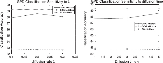
GPD. The graph pattern diffusion kernel was implemented, as discussed in Section 9.5.1. The default parameter for the GPD kernel is a diffusion rate of λ =20% and the diffusion time τ = 5.
9.5.2.4 Experimental Results Here we present the results of our graph classification experiments. One round of experiments was performed to evaluate the methods based on exact subgraph mining, and another round of experiments were with approximate subgraph mining. For both subgraph mining methods, patterns were selected that were general graphs, trees, and paths.
A simple feature selection method is applied in order to identify the most discriminating frequent patterns. Using a simple statistical formula, PCC, the correlation is measured between a set of feature samples (in our case, the occurrences of a particular subgraph in each of the data samples) and the corresponding class labels. Frequent patterns are ranked according to correlation strength, and the top 10% patterns are selected to construct the feature set.
Comparison between Classifiers. The results of the comparison of different graph kernel functions are shown in Table 9.5. For these results, frequent subgraph mining using exact matching was used. In the table that uses general subgraphs (the first 10 rows in Table 9.5), it is shown that for exact mining of general subgraphs, in 4 of the 10 data sets, the GPD method provides mean accuracy that is significantly better (at least two standard deviations above the next best method). In another, 4 data sets, GPD gives the best performance, but the difference is less significant and is still 1 standard deviation). In the last two data sets, other methods perform better, but not significantly better. The mismatch and min–max kernels all give roughly the same performance. Hence, only the results of the mismatch kernel are shown. The GPD′s superiority is also confirmed in classifications where tree and path patterns are used.
Table 9.6 compares the performance of our GPD kernel to the classification based on association (CBA) method. In general it shows comparable performance to the other methods. In one data set, it does show a noticeable increase over the other methods. This is expected since CBA is designed specifically for discrete data such as the binary feature occurrences used here. Despite the strengths of CBA, the GDA method still gives the best performance for six of the seven data sets. These data sets were also tested using the recursive optimal-assignment kernel included in the JOELib2 computational chemistry library. It’s results are comparable to those of the CBA method, and hence were not included here as separate results.
TABLE 9.5 Comparison of Different Graph Kernel Functions and Feature Sets in GPD Experiments, With Strict Subgraph Matching
In addition, a classifier called XRules was tested. XRules is designed for classification of tree data [13]. Chemical graphs, while not strictly trees, often are close to trees. To run the XRules executable, a graph is transformed to a tree by randomly selecting a spanning tree of the original graph. Our experimental study shows the application of XRules on average delivers incompetent results among the group of classifiers (e.g., 50% accuracy on the CDK2 inhibitor data set), which may be due to the particular way a graph is transformed to a tree. Since tree patterns are computed for the rule based classifier CBA in our comparison, XRules was not explored further.
A method based on a recursive optimal assignment [10] was also tested using biologically relevant chemical descriptors labeling each node in a chemical graph. In order to perform a fair comparison with this method to the other methods, the chemical descriptors are ignored and the focus is instead on the structural alignment. In these experiments, the performance of this method is very similar to CBA. Hence, only the results of CBA are shown here.
Comparison between Descriptor Sets. Various types of subgraphs (e.g., trees, paths, and cycles) have been used in kernel functions between chemical compounds. In addition to exact mining of general subgraphs, approximate subgraph mining was also used to generate the features for our respective kernel methods. In both cases, the general subgraphs mined are filtered into sets of trees and sets of paths as well.
The results for all kernels using exact tree subgraphs are identical to those for exact general subgraphs. This is not surprising, given that most chemical fragments are structured as trees. The results using exact path subgraphs, however, do show some shifts in accuracy, but the difference is not significant. These results are not recorded here since they add no appreciable information to the evaluation of the various methods.
The results using approximate subgraph mining (shown in Table 9.7) are similar to those for exact subgraph mining (shown in Table 9.5). In contrast to the hypothesis that using approximate subgraph mining might improve the classification accuracy, the data show that there is no significant difference between the set of features. However, it is clear that GPD is still better than the competing kernel functions.
TABLE 9.6 Comparison of GPD Kernel to CBA

TABLE 9.7 Comparison of Different Graph Kernel Functions and Feature Sets in GPD Experiments, With Approximate Subgraph Matching
Effect of Varying GPD Diffusion Rate and Time. This section evaluates the sensitivity of the GPD methods to its two parameters: diffusion rate λ and diffusion time. Different diffusion rate λ values and diffusion time values were tested. Figure 9.8 shows that the GPD algorithm is not very sensitive to the two parameters at the range that was tested. Although only three data sets are shown in Figure 9.8, the observation is true for other data sets in the experiments.
FIGURE 9.8 Effect of diffusion rate and time on GPD classification accuracy. From with permission.
9.5.3 Conclusions
With the rapid development of fast and sophisticated data collection methods, data has become complex, high-dimensional, and noisy. Graphs have proven to be powerful tools for modeling complex, high-dimensional, and noisy data; building highly accurate predictive models for graph data is a new challenge for the data-mining community. This work demonstrates the utility of a novel graph kernel function, graph pattern diffusion kernel (GPD kernel). It is shown that the GPD kernel can capture the intrinsic similarity between two graphs and has the lowest testing error in many of the data sets evaluated. Although a very efficient computational framework was developed, computing a GPD kernel may be hard for large graphs. Future work will concentrate on improving the computational efficiency of the GPD kernel for very large graphs, as well as performing additional comparisons between this method and other two-dimensional (2D)-descriptor and QSAR-based methods.
9.6 MATCHING KERNELS WITH APPROXIMATE PATTERN-BASED FEATURES
This chapter expands on the GPD kernel presented in Chapter 8, by defining a similar kernel function that uses a matching-based set kernel instead of an alignment kernel. This method is termed a graph pattern matching (GPM) kernel. The advantage of this modification is that the GPM kernel, unlike GPD, is guaranteed to be positive semidefinite, and hence a true Mercer kernel. This algorithm was tested using 16 chemical structure data sets. The experimental results demonstrate that this method outperforms existing state-of-the-art methods with a large margin.
9.6.1 Graph Pattern Matching Kernel with Diffusion for Accurate Graph Classification
This section presents the design of a graph matching kernel with diffusion. The section begins by first presenting a general framework for graph matching. Then the pattern-based graph matching kernel is presented. Finally, a technique called “pattern diffusion” is discussed that significantly improves graph classification accuracy in practice.
9.6.1.1 Graph Matching Kernel To derive an efficient algorithm scalable to large graphs, a function Γ : V → Rn is used to map nodes in a graph to an n-dimensional feature space that captures not only the node label information, but also the neighborhood topological information around the node. If there is such a function Γ, the following graph kernel may be defined
where K can be any kernel function defined in the codomain of Γ. This function Km is called a graph matching kernel. The following theorem indicates that Km is symmetric and positive semidefinite, and hence a real kernel function.
Theorem 9.6.1 The graph matching kernel is symmetric and positive semidefinite if the function K is symmetric and positive semidefinite.
Proof sketch: The matching kernel is a special case of the R-convolution kernel and is hence positive semidefinite as proved in [45].
The kernel function can be visualized by constructing a weighted complete bipartite graph: connecting every node pair ![]() with an edge. The weight of the edge (u, v) is K (Γ(v), Γ(v)). Figure 9.6 shows a weighted complete bipartite graph for V[G] = {v1, v2, v3} and V[G′] = {u1, u2, u3}. Highlighted edges (v1,u2), (v2,u1), (v3,u3) have larger weights than the rest of the edges (dashed).
with an edge. The weight of the edge (u, v) is K (Γ(v), Γ(v)). Figure 9.6 shows a weighted complete bipartite graph for V[G] = {v1, v2, v3} and V[G′] = {u1, u2, u3}. Highlighted edges (v1,u2), (v2,u1), (v3,u3) have larger weights than the rest of the edges (dashed).
We can see from the figure that if two nodes are quite dissimilar, the weight of the related edge is small. Since dissimilar node pairs usually outnumber similar node pairs, if a linear kernel is used for nodes, the kernel function may be noisy, and hence lose the signal. In this design, the RBF kernel function is used, as specified below, to penalize dissimilar node pairs.
where ||X||22 is the squared L2 norm of a vector X.
9.6.1.2 Graph Pattern Matching Kernel One way to design the function Γ is to take advantage of frequent patterns mined from a set of graphs. Intuitively, if a node belongs to a subgraph F, there is some information about the local topology of the node. Following the intuition, given a node v in a graph G and a frequent subgraph F, a function ΓF is designed such that
The function ΓF is called a “pattern membership function” since this function tests whether a node occurs in a specific subgraph feature (membership to a subgraph).
Given a set of frequent subgraphs F = F1, F2, …, Fn, each membership function is treated as a dimension and the function ΓF is defined as
In other words, given an n frequent subgraph, the function Γ maps a node v in G to an n-dimensional space, indexed by the n subgraphs, where values of the features indicate whether the node is part of the related subgraph in G.
Example 9.2 Figure 9.9, showns that two subgraph features, F1 and F2, where F1 is embedded in Q at q1, q2 and F2 occurs in Q at q1, q3. The occurrences are depicted using shadings with different color and orientations. For node q1, a subgraph F1 is considered as a feature, and ΓF1(q1) = 1 since q1 is part of an embedding of F1 in Q. Also, ΓF1(q3) = 0 since q3 is not part of an embedding of F1 in Q. Similarly, ΓF2(q1) = 1 and ΓF2(q3) = 1. Hence, ΓF1, F2(q1) = (1, 1) and ΓF1, F2(q3) = (0, 1). The values of the function ΓF1, F2 are also illustrated in the same figure using the annotated Q.
FIGURE 9.9 Example pattern membership functions for GPM kernel. From

9.6.1.3 Graph Pattern Matching Kernel with Pattern Diffusion This section introduces a better technique than the pattern membership function to capture the local topology information of nodes. This technique is called “pattern diffusion”. The design here has the following advantages:
It is generic and does not assume any domain knowledge from a specific application. The diffusion process may be applied to graphs with dramatically different characteristics.
The diffusion process is straightforward to implement and can be computed efficiently.
It is proof that the diffusion process is related to the probability distribution of a graph random walk. This explains why the simple process may be used to summarize local topological information.
Below, the pattern diffusion kernel is outlined in three steps.
In the first step, a seed is identified as a starting point for the diffusion. In this design, a “seed” could be a single node, or a set of connected nodes in the original graph. In the experimental study, frequent subgraphs are always used for seeds since a seed from one graph can be easily compared to a seed in another graph.
In the second step, given a set of nodes S as seed, a diffusion function ft is recursively defined in the following way:
The base f0 is defined as
Define ft+1 (t ≥ 0) with ft in the following way:
In the notation, ![]() is the set of nodes that connects to v directly and
is the set of nodes that connects to v directly and ![]() is the node degree of v. The parameter λ controls the diffusion rate.
is the node degree of v. The parameter λ controls the diffusion rate.
Equation (9.17) describes a process where each node distributes a λ fraction of its value to its neighbors evenly and in the same way receives some value from its neighbors. It is called “diffusion” because the process simulates the way a value is spreading in a network. The intuition is that the distribution of such a value encodes information about the local topology of the network.
To constrain the diffusion process to a local region, one parameter called diffusion time, denoted by τ, is used to control the diffusion process. Specifically, the diffusion process is limited to a local region of the original graph with nodes that are at most τ hops away from a node in the seed S. In this sense, the diffusion should be named “local diffusion”.
Finally, in the last step for the seed S, define the mapping function ΓdS as the limit function of ft as t approaches to infinity, or
And given a set of frequent subgraph F = F1, F2, …, Fn as seeds, define the pattern diffusion function ![]()
9.6.1.4 Connections of Other Graph Kernels Connection to Marginalized Kernels. Here the connection of pattern matching kernel function to the marginalized graph kernel [28] is shown, which uses a Markov model to randomly generate walks of a labeled graph.
Given a graph G with nodes set ![]() , and a seed S ⊆ V[G], for each diffusion function ft, construct a vector
, and a seed S ⊆ V[G], for each diffusion function ft, construct a vector ![]() . According to the definition of
. According to the definition of ![]() × Ut, where the matrix M is defined as
× Ut, where the matrix M is defined as
In this representation, compute the stationary distribution ![]() by computing M∞ × U0.
by computing M∞ × U0.
Note that the matrix M corresponds to a probability matrix corresponding to a Markov chain since
- All entries are non-negative.
- Column sum is 1 for each column.
Therefore the vector M∞ × U0 corresponds to the stationary distribution of the local random walk as specified by M. In other words, rather than using random walk to retrieve information about the local topology of a graph, the stationary distribution is used to retrieve information about the local topology. The experimental study shows that this in fact is an efficient method of graph classification.
Connection to Optimal Assignment Kernel. The optimal assignment (OA) kernel [34] carries the same spirit of the graph pattern matching kernel in that OA uses pairwise node kernel function to construct a graph kernel function. The OA kernel has been utilized for cheminformatics applications and is found to deliver good results empirically.
There are two major differences between GPM and the OA kernel. (1) The OA kernel is not positive semidefinite, and hence is not a Mercer kernel in a strict sense. Non-Mercer kernel functions are used to train SVM models and the problem is that the convex optimizer utilized in SVM will not converge to a global optimal and hence the performance of the SVM training may not be reliable. (2) The OA utilizes a complicated recursive function to compute the similarity between nodes, which make the computation of the kernel function run slowly for large graphs [10].
9.6.1.5 Pattern Diffusion Kernel and Graph Classification This section summarizes the discussions presented so far and shows how the kernel function is utilized to construct an efficient graph classification algorithm in both the training and testing phases.
Training Phase. In the training phase, graphs of the training data set ![]() are divided into groups according to their class labels. For example in binary classification there are two groups of graphs: positive or negative. For multiclass classification, graphs are partitioned according to their class label, where graphs having the same class labels are grouped together. The training phase is composed of four steps:
are divided into groups according to their class labels. For example in binary classification there are two groups of graphs: positive or negative. For multiclass classification, graphs are partitioned according to their class label, where graphs having the same class labels are grouped together. The training phase is composed of four steps:
1. Obtain frequent subgraphs. Identify frequent subgraphs from each graph group and union the subgraph sets together as the seed set F.
2. For each graph G in the training data set, use the node pattern diffusion function ΓdF to label nodes in G. Thus the feature vector of a node v is a vector ![]() with length m = |F|.
with length m = |F|.
3. For two graphs G, G′, construct the complete weighted bipartite graph as described in Section 9.6.1.1 and compute the kernel Km(G, G′) using Eqs. (9.14) and (9.15).
4. Train a predictive model using a kernel classifier.
Testing Phase. In the testing phase, the kernel function is computed for graphs in the testing and training data sets. The trained model is used to make predictions about graph in the testing set.
- For each graph G in the testing data set, use ΓdF to label nodes in G and create feature vectors as in the training phase.
- Use Eqs. (9.14) and (9.15) to compute the kernel function
- Km(G, G′) for each graph G in the testing data set and for each graph G′ in the training data set.
- Use kernel classifier and trained models to obtain prediction accuracy of the testing data set
9.6.5 Experimental Study
Classification experiments were conducted using six different graph kernel functions, including the pattern diffusion kernel, on 16 different data sets. There are 12 chemical–protein binding data sets, and the rest are chemical toxicity data sets. All of the experiments were performed on a desktop computer with a 3-GHz Pertium 4 processor and 1 GB of RAM. The following sections describe the data sets and the classification methods in more detail along with the associated results.
In all classification experiments, the LibSVM [44] was used as kernel classifier. The nu-SVC was used with default parameter ν = 0.5. The classification accuracy (TP+TN/S, TP: true positive, TN: true negative, S: total number of testing samples) is computed by averaging over a 10-fold cross-validation experiment. Standard deviation is computed similarly. To have a fair comparison, default SVM parameters were used in all cases, and were not tuned to increase the accuracy of any method.
9.6.2.1 Data Sets Sixteen data sets were selected, covering prediction of chemical–protein binding activity and chemical toxicity. The first seven data sets are manually extracted from the BindindDB database [45]. The next five are established data sets taken from Jorissen and Gilson [38]. The last four are from the predictive toxicology challenge [35] (PTC). Detailed information for the data sets is available in Table 9.8 where no. G-number of samples (chemical compounds) in the data set, no. P-positive samples, and no. N-negative samples.
TABLE 9.8 Characteristics of Data Sets in GPM Experiments
BindingDB Sets. The BindingDB database contains >450 proteins. For each protein, the database record chemicals that bind to the protein. Two types of activity measurements Ki and IC50 are provided. Both measurements measure inhibition–dissociation rates between a proteins and chemicals. From BindingDB, 7 proteins were manually selected with a wide range of known interacting chemicals (ranging from tens to several hundreds). These data sets are AChE, ALF, EGF-R, HIV-P, HIV-RT, HSP90, and MAPK.
Jorissen Sets. The Jorissen data sets also contains information about chemical–protein binding activity. In this case, the provider of the data set carefully selected positive and negative samples, and hence is more reliable than the data sets created from BindingDB. For more information about the creation of the data sets, see [38] in details. The data sets from this study are CDK2, COX2, FXa, PDE5, and A1A.
PTC Sets. The PTC data sets contain a series of chemical compounds classified according to their toxicity in male and female rats and male and female mice. While chemical–protein binding activity is an important type of chemical activity, it is not the only type. Toxicity is another important, though different, kind of chemical activity necessary to predict in drug design. These data sets (PTC–FR/FM/MR/MM) are well curated and highly reliable.
9.6.2.2 Kernel Functions Six different kernel functions were selected for evaluation: marginalized [28], spectrum [24], tanimoto [26], subtree [33], optimal assignment [34], together with the graph pattern matching kernel.
Four kernel functions (marginalized, spectrum, tanimoto, and subtree) are computed using the open source Chemcpp v1.0.2 package [47]. The optimal assignment kernel was computed using the JOELib2 package, and is not strictly a kernel function, but still provides good prediction accuracy. The graph pattern matching kernel was computed using MATLAB code.
9.6.2.3 Experimental Results Comparison between Kernel Functions. This section presents the results of our graph classification experiments with various kernel functions. Figure 9.10 shows the classification accuracy for different kernel functions and data sets, averaged over a 10-fold cross-validation experiment. The standard deviations (omitted) of the accuracies are generally very high, from 5–10%, so statistically significant differences between kernel functions are generally not observed.
FIGURE 9.10 Average accuracy for kernel functions and data sets in GPM experiments. From
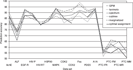
The data shows that the GPM method is competitive for all 16 data sets. If the accuracy of each kernel function averaged over all data sets is examined, the GPM kernel performs the best overall. Again, the standard deviations are high so the differences between the top performing kernels are not statistically significant. Still, with 16 different data sets some trends are clear: GPM kernel delivers the highest classification accuracy in 8 out of the 16 data sets, with tanimoto kernel best in 4, marginalized best in 2, subtree in 2, optimal assignment in 1, and spectrum in none.
Although GPM does not work well on a few data sets (e.g., AChE, HIV–RT, MAPK, and PTC–FR/MR), overall it performs better when compared to any other kernels for a majority of data sets. It is better than every other kernel function in at least 10 of the 16 data sets.
In general the GPM, spectrum and tanimoto kernels perform the best, with an overall average accuracy of ∼80%. The subtree, optimal assignment, and marginalized also perform very good, in the mid to high 70%. The min–max tanimoto kernel performed much worse than the other methods, and hence were not included in the figure. Note that the optimal assignment kernel is missing a prediction accuracy for the FXa data set, which was due to a terminal error in the JOELib2 software used to calculate this kernel on this data set.
9.6.3 Conclusions
Graphs have proven to be powerful tools for modeling complex and high-dimensional biological data; building highly accurate predictive models for chemical graph classification is a goal for cheminformatics and drug design. This work demonstrates the utility of a novel graph kernel function, graph pattern matching kernel (GPM kernel). It is shown that the GPM kernel can capture the intrinsic connection between a chemical and its class label and has the lowest testing error in a majority of the data sets we evaluated.
9.7 GRAPH WAVELETS FOR TOPOLOGY COMPARISON
Previous kernels such as the alignment kernel or other substructure-based kernels attempt to mitigate the high-dimensionality of graphs in different ways. The first possibility is to use complex patterns (e.g., general subgraphs), but restrict pattern selection in some way. The second approach is to use simpler patterns (e.g., paths or trees), but retain the set of feature patterns. In the most extreme case, graphs are reduced to point sets of vertices for very fast but information-poor analysis. The approach presented here, termed Wavelet–Alignment (WA) kernel, works on simpler graph representations, but uses an application of graph wavelet analysis to create high-quality localized structure features for chemical analysis. The wavelet functions are used to condense neighborhood information about an atom into a single feature of that atom, rather than features spread over it’s neighboring atoms. By doing so, (local) features are extracted with various topological scales about chemical structures and these wavelet features can be used to compute an alignment of two chemical graphs. This chapter describes the wavelet-alignment method in detail and compares it to competing methods for chemical activity prediction with several data sets.
9.7.1 Graph Wavelet Alignment Kernels for Drug Virtual Screening
The following sections outline the algorithms that drive our experimental method. This method measures the similarity of graph structures whose nodes and edges have been labeled with various features. These features represent different kinds of chemical structure information including atoms and chemical bond types, among others. To compute the similarity of two graphs, the nodes of one graph are aligned with the nodes of the second graph, such that the total overall similarity is maximized with respect to all possible alignments. Vertex similarity is measured by comparing vertex descriptors, and is computed recursively so that when comparing two nodes, the immediate neighbors of those nodes are also compared, and the neighbors of those neighbors, and so on.
9.7.1.1 Graph Alignment Kernel An alignment of two graphs G and G′ (assuming is a 1-1 mapping. Given an alignment π, define the similarity between two graphs, as measured by a kernel function kA, below:
The function kn is a kernel function to measure the similarity of nodes and the function ke is a kernel function to measure the similarity of edges. Intuitively, Eq. (9.20) uses an additive model to compute the similarity between two graphs by computing the sum of the similarity of nodes and the similarity of edges. The maximal similarity among all possible alignments is defined as the similarity between two graphs.
9.7.1.2 Simplified Graph Alignment Kernel A direct computation of the graph alignment kernel is computationally intensive and is unlikely scalable to large graphs. With no surprise, the graph alignment kernel computation is no easier than the subgraph isomorphism problem, a known NP-hard problem. (Formally, showing a reduction from the graph alignment kernel to the subgraph isomorphism problem is needed. The details of such reduction are omitted due to their loose connection to the main theme of the current paper, which is an advanced data-mining approach, as applied to cheminformatics applications.) To derive efficient algorithms scalable to large graphs, the graph kernel function is simplified with the following formula:
Where π: V[G] → V[G′] denotes an alignment of graph G and G′. The parameter f(v) is a set of features associated with a node that not only include node features, but also include information about topology of the graph where v belongs.
Equation (9.21), computes a maximal weighted bipartite graph, which has an efficient solution known as the Hungarian algorithm. The complexity of the algorithm is O(|V[G]|3). See [34] for further details.
Provided below is an efficient method, based on graph wavelet analysis, to create features to capture the topological structure of a graph.
9.7.1.3 Graph Wavelet Analysis Originally proposed to analyze time series signals, wavelet analysis transforms a series of signals to a set of summaries with different scale. Two of the key insights of wavelet analysis of signals are (1) using localized basis functions and (2) analysis with different scales. Wavelet analysis offers efficient tools to decompose and represent a function with arbitrary shape [47,48]. Since invented, wavelet analysis has quickly gained popularity in a wide range of applications outside time series data, (e.g., image analysis and geography data analysis). In all these applications, the level of detail, or scale, is considered as an important factor in data comparison and compression. Figure 9.11 shows two examples of wavelet functions in a 3D space, the Haar and Mexican Hat.
FIGURE 9.11 Two wavelet functions in three dimensions (3 Ds), Mexican hat and Haar. From

Intuition. With wavelet analysis, as applied to graph representations of chemical structure features about each atom and its local environment are collected at different scales. For example, information can be collected about the average charge of an atom and it’s surrounding atoms, then assign the average value as a feature to the atom. Information can also be collected about whether an atom belongs to a nearby functional group, whether the surrounding atoms of a particular atom belong to a nearby functional group, and the local topology of an atom to its nearby functional groups.
In summary, conceptually the following two types of insights are gained about the chemicals after applying wavelet analysis to graph represented chemical structure:
1. Analysis With Varying Levels of Scale. Intuitively, at the finest level, two chemical structures are compared by matching the atoms and chemical bonds in the two structures. At the next level, comparison of two regions is performed (e.g., chemical functional groups). At an even coarser level, small regions may be grouped into larger ones (e.g., pharmacophore), and two chemicals are compared by matching the large regions and the connections among large regions.
2. Nonlocal Connection. In a chemical structure, two atoms that are not directly connected by a chemical bond may still have some kind of interaction. Therefore when comparing two graphs, their vertices cannot depend only on the local environment immediately surrounding an atom, but rather must consider both the local and nonlocal environment.
Though conceptually appealing, current wavelet analysis is often limited to numerical data with regular structures (e.g., matrices and images). Graphs, however, are arbitrarily structured and may represent innumerable relationships and topologies between data elements. In order to define a reasonable graph wavelet function, the following two important concepts are introduced (1) h-hop neighborhood and (2) discrete wavelet functions.
The former (h-hop neighborhood) is essentially used to project graphs from a high-dimensional space with arbitrary topology into a Euclidean space suitable for operation with wavelets. The h-hop measure defines a distance metric between vertices that is based on the shortest path between them. The discrete wavelet function then operates on a graph projection in the h-hop Euclidean space to compactly represent the information about the local topology of a graph. It is the use of this compact wavelet representation in vertex comparison that underlies the complexity reduction achieved by this method. Based on the h-hop neighborhood, a discrete wavelet function is used to summarize information in a local region of a graph and create features based on the summarization. These two concepts are discussed in detail below.
h-hop Neighborhood. In this section, the following definitions are introduced.
Definition 9.7.1 Given a node v in a graph G the h-hope neighborhood of v, denoted by Nh(v), is the set of nodes that are (according to the shortest path) exactly h-hops away from v.
For example if h = 0, then ![]() .
.
Here, fv denotes the feature vector associated with a node v in a graph G. The parameter |f| is the feature vector length (number of features in the feature vector). The average feature measurement, denoted by ![]() for nodes in Nj(v), is
for nodes in Nj(v), is
Example 9.3 Figure 9.5(a) shows a chemical graph. Given a node v in the graph G, label the shortest distance of nodes to v in G. In this case, N0(v) = v and N1(v) = {t,u}. If the feature vector contains a single feature of atomic number, ![]() is the average atomic number of atoms that are at most 1-hop away from v. In this case, since N1(v) = {t,u} and {t,u} are both carbon with an atomic number equal to eight, then
is the average atomic number of atoms that are at most 1-hop away from v. In this case, since N1(v) = {t,u} and {t,u} are both carbon with an atomic number equal to eight, then ![]() is equal to eight as well.
is equal to eight as well.
Discrete Wavelet Functions. In order to adapt a wavelet function to a discrete structure (e.g., graphs), a wavelet function ψ(x) must be applied to the h-hop neighborhood. Toward that end, a wavelet function ψ(x) (e.g., the Haar or Mexican Hat) can be scaled to have support on the domain [0,1), with integral 0, and partition the function into h+1 intervals. Then, compute the average, ψj,h, as the average of ψ(x) over the jth interval, 0 ≤ j ≤ h as
With neighborhood and discrete wavelet functions, wavelet analysis can be applied to graphs. This analysis is called wavelet measurements, denoted by Γh(v), for a node v in a graph G at scale up to h > 0.
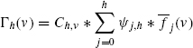
where Ch,v is a normalization factor with ![]()
Define Γh(v) as the sequence of wavelet measurements as applied to a node v with scale value up to h. That is Γh(v) = {Γ1(v), Γ2(Γhv), … , Γh(v)}. Call Γh(v) the wavelet measurement vector of node v. Finally insert the wavelet measurement vector into the alignment kernel with the following formula:
where ka(Γh(v), Γh(π(v)) is a kernel function defined on vectors. Two popular choices are linear kernel and radius-based function kernel.
Example 9.4 Figure 9.5(b) shows a chemical graph overlayed with a wavelet function centered on a specific vertex. It is clear how the wavelet is most intense at the central vertex, hop distance of zero, corresponding to a strongly positive region of the wavelet function. As the hop distance increases, the wavelet function becomes strongly negative, roughly at hop distances of one and two. At hop distance >2, the wavelet function returns to zero intensity, indicating negligible contribution from vertices at this distance.
9.7.2 Experimental Study
Classification experiments were conducted on five different biological activity data sets, and measured SVM classifier prediction accuracy for several different feature generation methods. The following sections describe the data sets and classification methods in more detail, along with the associated results.
We performed all experiments on a desktop computer with a 3-GHz Pertium 4 processor and 1 GB of RAM.
9.7.2.1 Data Sets Five data sets were selected to represent typical chemical benchmarks in drug design to evaluate the classifier performance. The PTC data set, discussed by Helma et al. [35], contains a set of chemical compounds classified according to their toxicity in male rats (PTC–MR), female rats (PTC–FR), male mice (PTC–MM), and female mice (PTC–FM). The human intestinal absorption (HIA) data set (Wessel et al. [36]) contains chemical compounds classified by intestinal absorption activity. The remaining data set (MD) is from Patterson et al. [40], and was used to validate certain molecule descriptors. Various statistics for these data sets can be found in Table 9.9.
TABLE 9.9 Data Set and Class Statistics for WA Experiments
All of these data sets exist natively as binary classification problems, therefore in the case of the MD and HIA data sets, some preprocessing is required to transform them into regression and multiclass problems. For regression, this is a straightforward process of using the compound activity directly as the regression target. In the case of multiclass problems, the transformation is not as direct. A histogram of compound activity values was chosen to visualize which areas of the activity space are more dense, allowing natural and intuitive placement of class separation thresholds.
9.7.2.2 Methods The performance of the SVM classifier trained with different methods was evaluated. The first two methods (WA–linear, WA–RBF) are both computed using the wavelet-alignment kernel, but use different functions for computing atom–atom similarity; both a linear and RBF function were tested here. Different hop distance thresholds were evaluated and fixed to h=3 in all experiments.
The method OA consists of the similarity values computed by the optimal assignment kernel, as proposed by Frölich et al. [34]. There are several reasons that we consider OA as the current state-of-the-art graph-based chemical structure classification method. First, the OA method is developed specifically for chemical graph classification. Second the OA method contains a large library to compute different features for chemical structures. Third, the OA method has developed a sophisticated kernel function to compute the similarity between two chemical structures. The experimental study shows that the wavelet analysis obtains performance profiles comparable to, and sometimes exceeding that of the existing state-of-the-art chemical classification approaches. In addition, a significant computation time reduction was achieved by using the wavelet analysis. The details of the experimental study are shown below.
In these experiments, the SVM classifier was used in order to generate activity predictions. The LibSVM classifier was used, as implemented by Chang et al. [43] and included in the Weka data-mining software package by Witten et al. [42]. The SVM parameters were fixed across all methods, and we use a linear kernel. For (binary) classification, nu-SVC was used for multiclass classification with nu = 0.5. The Haar wavelet function was used in the WA experiments. Classifier performance was averaged over a 10-fold cross-validation set.
Most of the algorithms were developed and tested under the MATLAB programming environment. The OA software was provided by [34] as part of their JOELib software, a computational chemistry library implemented in java [23]
9.7.2.3 Results Below are results of the experimental study of the wavelet-alignment kernel with two focuses: (1) classification accuracy and (2) computational efficiency.
TABLE 9.10 Prediction Results of Cross-Validation Trials for WA Experiments
9.7.2.4 Classification Accuracy Table 9.10 reports the average and standard deviation of the prediction results over 10 trials. The best results are marked with an asterisk. For classification problems, results are in prediction accuracy, and for regression problems they are in mean-squared-error (MSE) per sample. From the table, observe that for the HIA data set, WA–RBF kernel significantly outperforms OA for both binary and multiclass classification. For the MD data set, OA does best for both classification sets, but WA–linear is best for regression. For the PTC binary data, the WA–linear method outperforms the others in three of the four sets.
9.7.2.5 Computational Efficiency In Table 9.11, the kernel computation time for both OA and WA methods was documented using six different data sets. The runtime advantage of the WA algorithm over OA is clear, showing improved computation efficiency by factors of > 10-fold for the WA–linear kernel and over fivefold for the WA–RBF kernel.
Figure 9.12 shows the kernel computation time across a range of data set sizes, with chemical compounds sampled from the HIA data set. Using simple random sampling with replacement, data sets were created sized from 50 to 500. The OA method was not run on even larger data sets since the experimental results clearly demonstrate the efficiency of the WA kernel already.
TABLE 9.11 Running Time Results for WA Experiments
FIGURE 9.12 Comparison of computation times between methods for WA experiments. From cite{Smalter08d}, with permission.
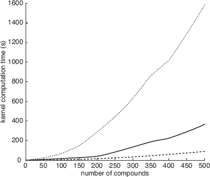
What these run time results do not demonstrate is the even greater computational efficiency afforded by the WA algorithm when operating on general, non-chemical graph data. Chemical graphs have some restrictions on their general structure, specifically, the number of atom neighbors is bound by a small constant (4 or so). Since the OA computation time is much more dependent on the number of neighbors, WA is even more advantageous in these circumstances. Unfortunately, since the OA software is designed as part of the JOELib chemoinformatics library specifically for use with chemical graphs, it will not accept generalized graphs as input, and hence this aspect of the algorithm could not be empirically demonstrated
9.7.3 Conclusions
Graph structures are a powerful and expressive representation for chemical compounds. This work presents a new method wavelet-assignment, for computing the similarity of chemical compounds, based on the use of an optimal assignment graph kernel function augmented with pattern and wavelet-based descriptors. The experimental study demonstrates that this wavelet-based method delivers an improved classification model, along with an order of magnitude speedup in kernel computation time. For high-volume, real-world data sets, this algorithm is able to handle a much greater number of graph objects, demonstrating it’s potential for processing both chemical and non-chemical data in large amounts. In the present study, only a limited number of atom features are used. In the future, domain experts can be involved to evaluate the performance of these algorithms, including the prediction accuracy and the capability for identifying important features in diverse chemical structure data sets.
9.8 CONCLUSIONS
Graph structures are a powerful and expressive representation for many kinds of data. With the rapid development of fast and sophisticated data collection methods, data has become complex, high-dimensional, and noisy. Graphs have proven to be powerful tools for modeling such data.
Building highly accurate predictive models for graph data is a new challenge for the data mining and machine learning communities. These methods are of great value in a variety of fields, but especially so in biological and chemical research where computational tools are helping to make many important new discoveries with respect to disease treatment and other medical activities.
Much recent activity on graph classification has focused on the definition of kernel functions for comparing graph objects directly. The kernel function defines an implicit feature space where graph classification can be accomplished via support vector machine or another kernel classifier. Classification in kernel space avoids many difficulties associated with using high-dimensional feature vectors to represent graphs and other complex objects.
The use of kernel functions do not completely mitigate the problems of working with complex graph objects, however. Currently established kernel functions are either slow to compute or lack discriminative power. This chapter addresses these issues through several novel techniques, however, there remain many opportunities for further improvement. In the chemical domain, at least, there appear to be many high-level structural rules that even complex models have difficulty capturing. The most precise models are prohibitively time consuming for databases of the size now available.
Future work must focus on methods for efficient, large-scale analysis. The value of this high-volume approach is exemplified by the proliferation of high-throughput screening technology, which has drastically accelerated the analysis of chemicals and biological molecules. The ability to accurately and quickly analyze databases in the millions of compounds using only computer models offers unprecedented opportunities for learning about biological systems.
Ultimately, the result of improved computer models is a better understanding and control of complex phenomena. Biological systems, though an important beneficiaries of such models, are only a single area of potential application. Graphs are fundamental to our general understanding of many concepts. Therefore, only by fully understanding graphs can these concepts themselves be fully modeled and understood.
REFERENCES
1. N. Tolliday, P. A. Clemons, P. Ferraiolo, A. N. Koehler, T. A. Lewis, X. Li, S. L. Schreiber, D. S. Gerhard, and S. Eliasof (2006), Small molecules, big players: the national cancer institute’s initiative for chemical genetics. Cancer Res., 66:8935–8935.
2. C. P. Austin, L. S. Brady, T. R. Insel, and F. S. Collins (2004), Nih molecular libraries initiative. Science, 306(5699):1138–1139.
3. Y. Xue, H. Li, C. Y. Ung, C. W. Yap, and Y. Z. Chen (2006), Classification of a diverse set of tetrahymena pyriformis toxicity chemical compounds from molecular descriptors by statistical learning methods. Chem. Res. Toxicol., 19 (8).
4. R. Put, Q. S. Xu, D. L. Massart, and Y. V. Heyden (2004), Multivariate adaptive regression splines (mars) in chromatographic quantitative structure-retention relationship studies. J Chromatogr A., 1055(1–2).
5. V. Svetnik, A. Liaw, C. Tong, J. C. Culberson, R. P. Sheridan, and B. P. Feuston (2003), Random forest: A classification and regression tool for compound classification and qsar modeling. J. Chem. Information Computer Sci., 43
6. D. Haussler (1999), Convolution kernels on discrete structures. Technical Report UCSC-CRL099-10, Computer Science Department, UC Santa Cruz.
7. A. Smalter, J. Huan, and G. Lushington (2008), Structure-based pattern mining for chemical compound classification. Proceedings of the 6th Asia Pacific Bioinformatics Conference, Kyato, Japan.
8. A. Smalter, J. Huan, and G. Lushington (2008), Gpd: A graph pattern diffusion kernel for accurate graph classification. Proceedings of the 8th International Workshop on Data Mining in Bioinformatics, Las Vegas, NE.
9. A. Smalter, J. Huan, and G. Lushington (2008), Gpm: A graph pattern matching kernel with diffusion for accurate graph classification. Proceedings of the 8th IEEE International Conference on BioInformatics and BioEngineering, Athens, Greece.
10. A. Smalter, J. Huan, and G. Lushington (2009), Graph wavelet alignment kernels for drug virtual screening. J. Bioinformatics Computational Bio., 7:473–497.
11. M. Crovella and E. Kolaczyk (2003), Graph wavelets for spatial traffic analysis. Infocom, 3:1848–1857.
12. M. Maggioni, J. Bremer, Jr, R. Coifman, and A. Szlam (2005), Biorthogonal diffusion wavelets for multiscale representations on manifolds and graphs. Proc. SPIE Wavelet XI, Vol. 5914.
13. M. J. Zaki and C. C. Aggarwal (2006), Xrules: An effective structural classifier for xml data. Machine Learning J. Special Issue Stat. Relational Learning Multi-Relational Data Mining, 62(1–2):137–170.
14. B. Liu, W. Hsu, and Y. Ma (1998), Integrating classification and association rule mining. Proceedings of the Fourth International Conference on Knowledge Discovery and Data Mining, NY.
15. J. R. Quinlan (1993), C4.5 : Programs for Machine Learning. Morgan Kaufmann.
16. V. Vapnik (1998), Statistical Learning Theory. John Wiley & Sons, Inc. NY.
17. A. Inokuchi, T. Washio, and H. Motoda (2000), An apriori-based algorithm for mining frequent substructures from graph data. PKDD′00, Lyon, France, 13–23.
18. M. Kuramochi and G. Karypis (2001), Frequent subgraph discovery. Proc. International Conference on Data Mining’01, San Diego, CA, pp. 313–320.
19. X. Yan and J. Han (2002), gspan: Graph-based substructure pattern mining. Proc. International Conference on Data Mining’02, Masbashe City, Japan, 721–724.
20. W. Wang, J. Huan, and J. Prins (2003), Efficient mining of frequent subgraphs in the presence of isomorphism. In Proceeding of ICDM, Melbourne, FL.
21. J. Huan, W. Wang, J. Prins, and J. Yang (2004), SPIN: Mining maximal frequent subgraphs from graph databases, Seattle, WA, 581–586.
22. S. Nijssen and J. N. Kok (2004), A quickstart in frequent structure mining can make a difference. Proceedings of the 10th ACM SIGKDD International Conference on Knowledge Discovery and Data Mining, Seattle, WA, 647–652.
23. J. Huan, W. Wang, and J. Prins (2003), Efficient mining of frequent subgraph in the presence of isomorphism. Proceedings of the 3rd IEEE International Conference on Data Mining (ICDM), Melbourne, FL, pp. 549–552.
24. M. Deshpande, M. Kuramochi, and G. Karypis (2005), Frequent sub-structure-based approaches for classifying chemical compounds. IEEE Trans. on Knowledge Data Eng., 1768:1036–1050.
25. T. Kudo, E. Maeda, and Y. Matsumoto (2004), An application of boosting to graph classification. NIPS, Vancaurce, Canada.
26. L. Ralaivola, S. J. Swamidass, H. Saigo, and P. Baldi (2005), Graph kernels for chemical informatics. Neural Networks, 18:1093–1110.
27. T. Gärtner, P. Flach, and S. Wrobel (2003), On graph kernels: Hardness results and efficient alternatives. Sixteenth Annual Conference on Computational Learning Theory and Seventh Kernel Workshop, Washington, DC.
28. H. Kashima, K. Tsuda, and A. Inokuchi (2003), Marginalized kernels between labeled graphs. Proceedig of the Twentieth International Conference on Machine Learning (ICML), Washington, DC.
29. K. M. Borgwardt and H. P. Kriegel (2005), Shortest-path kernels on graphs. Proceeding of the International Conference on Data Mining, Houston, TX, 27–31, NY.
30. J. Ramon and T. Gärtner (2003), Expressivity versus efficiency of graph kernels. In Technical Report, First International Workshop on Mining Graphs, Trees and Sequences, Carat. Dubrounik, Groatia.
31. T. Horvath, T. Gartner, and S. Wrobel (2004), Cyclic pattern kernels for predictive graph mining. SIGKDD, Seattle, WA.
32. N. Wale, I. Watson, and G. Karypis (2007), Comparison of descriptor spaces for chemical compound retrieval and classification. Knowledge Infor. Systems, 14(3):347–375.
33. P. Mahe and J. P. Vert (2006), Graph kernels based on tree patterns for molecules. Technical Report HAL:ccsd-00095488, Ecoles des Mines de Paris.
34. H. Fröhlich, J. Wegner, F. Sieker, and A. Zell, (2006), Kernel functions for attriubted molecular graphs - a new similarity-based approach to adme prediction in classification. QSAR Combinatorial Sci., 25(4):317–326.
35. C. Helma, R. King, and S. Kramer (2001), The predictive toxicology challenge 2000–2001. Bioinformatics, 17(1):107–108.
36. M. Wessel, P. Jurs, J. Tolan, and S. Muskal (1998), Prediction of human intestinal absorption of drug compounds from molecular structure. J. Chem. Inf. Comput. Sci., 38(4):726–735.
37. F. Fontaine, M. Pastor, I. Zamora, and F. Sanz (2005), Anchor-grind: Filling the gap between standard 3d qsar and the grid-independent descriptors. J. Med. Chem., 48:2687–2694.
38. R. Jorissen and M. Gilson (2005), Virtual screening of molecular databases using a support vector machine. J. Chem. Inf. Model., 45(3):549–561.
39. D. Patterson, R. Cramer, A. Ferguson, R. Clark, and L. Weinberger (1996), Neighbourhood behaviour: A useful concept for validation of “molecular diversity” descriptors. J. Med. Chem., 39:3049–3059.
40. J. Platt (1998), Fast Training of Support Vector Machines using Sequential Minimal Optimization. MIT Press, Cambridge, MA.
41. I. Witten and E. Frank (2005), Data Mining: Practical machine learning tools and techniques, 2nd ed. Morgan Kaufmann, San Francisco, CA.
42. R. Ahuja, T. Magnanti, and J. Orlin (1995), Network flows, SIAM Rev., 37 (1).
43. C. Chang and C. Lin (2001), Libsvm: a library for support vector machines, Available at http://www.csie.ntu.edu.tw/cjlin/libsvm.
44. S. Lyu (2005), Mercer kernels for object recognition with local features. IEEE Computer Vision and Pattern Recognition, San Diego, CA, 223–229.
45. T. Liu, Y. Lin, X. Wen, R. N. Jorrisen, and M. K. Gilson (2007), Bindingdb: a web-accessible database of experimentally determined protein-ligand binding affinities. Nucleic Acids Res., 35:D198–D201.
46. J. L. Perret, P. Mahe, and J. P. Vert (2007), Chemcpp: an open source c++ toolbox for kernel functions on chemical compounds, Available at http://chemcpp.sourceforge.net.
47. A. Deligiannakis and N. Roussopoulos (2003), Extended wavelets for multiple measures. Proceedings of the 2003 ACM SIGMOD International Conference on Management of Data San Diego, CA.
48. M. Garofalakis and A. Kumar (2005), Wavelet synopses for general error metrics. ACM Tran. Database Systems (TODS), 30(4):888–928.