CHAPTER 12

IDENTIFYING POTENTIAL GENE MARKERS USING SVM CLASSIFIER ENSEMBLE

ANIRBAN MUKHOPADHYAY, UJJWAL MAULIK, AND SANGHAMITRA BANDYOPADHYAY

12.1 INTRODUCTION

An important task in modern data mining is to utilize advanced data analysis and integration tools in gene expression pattern discovery and classification. These tools include a number of machine learning techniques, which may help in identifying relevant features for diagnostic and system biology studies. Furthermore, discovery of novel automated techniques for intelligent information retrieval and knowledge representation are crucial for biological data analysis. When a living cell undergoes a biological process, not all of its genes are expressed at the same time. Function of a cell is critically related to the gene expression at a given time and their relative abundance. For understanding biological processes, it is usual to measure gene expression levels in different developmental phases, body tissues, clinical conditions, and organisms. This information of differential gene expression can be utilized in characterizing gene function, determining experimental treatment effects, and understanding other molecular biological processes. Traditional approaches to genomic research was based on examining and collecting data for a single gene locally. The progress in the field of microarray technology has made possible to the study of the expression levels of a large number of genes across different time points or tumor samples [1–5]. Microarray technology has its application in a wide variety of fields, including medical diagnosis and cancer classification. Supervised classification is usually used to classify the tissue samples into two classes, namely, normal (benign) and cancerous (malignant) or into their subclasses, considering the genes as classification features [6–9]. For successful diagnosis and treatment of cancer, it is important to have a precise and reliable classification of tumors. Classical methods for classifying human malignancies rely on various morphological, clinical, and molecular variables. In spite of recent progress, there are still uncertainties in diagnosis. Also, it is likely that the existing classes are heterogeneous and comprise diseases that are molecularly distinct and follow different clinical courses. Deoxyribonucleic acid (DNA) microarrays may be used to characterize the molecular variations among tumors by monitoring gene expression profiles on a genomic scale. This leads to a finer and more reliable classification of tumors, which in turn helps to identify marker genes that distinguish among these classes. Eventually this improves the ability to understand and predict cancer survival. There are several classification approaches studied by bioinformatics researchers, among which support vector machine (SVM) classifier [10,11] has been widely used for this purpose [12–18]. The SVMs are powerful classification systems based on regularization techniques and provide excellent performance in many practical classification problems.

In this chapter, we have employed a SVM classifier to analyze a microarray matrix. The SVM classifiers use different kernel functions of which, four kernel functions, namely, linear, polynomial, sigmoidal, and radial basis function (RBF) are used. As different kernel functions can produce different classification results even when they are trained by the same set of samples, in this study we have used a majority voting ensemble technique to combine the classification results of the different kernel functions. Subsequently, this classification result is utilized to identify relevant gene markers based on SNR statistics followed by a feature selection method based on multiobjective genetic algorithm [19–21].

The performance of the proposed technique has been demonstrated on three publicly available benchmark cancer data sets, namely, leukemia, colon cancer, and lymphoma data. The experimental results establish the utility of the proposed ensemble classification technique. Moreover, relevant gene markers are identified from the four data sets that are responsible for different types of cancer.

12.2 MICROARRAY GENE EXPRESSION DATA

A microarray is typically a glass (or some other material) slide, on to which DNA molecules are attached at fixed locations (spots) [22]. There may be tens of thousands of spots on an array, each containing a huge number of identical DNA molecules (or fragments of identical molecules), of lengths from 20 to hundreds of nucleotides. Each of these molecules ideally should identify one gene or one exon in the genome. The chip is made of chemically coated glass, nylon, membrane, or silicon. Each grid cell of a microarray chip corresponds to a DNA sequence. For a cyclic DNA (cDNA) microarray experiment, the first step is to extract ribonucleic acid (RNA) from a tissue sample and amplification of RNA. Thereafter two messenger RNA (mRNA) samples are reverse transcribed into cDNA (targets) labeled using different fluorescent dyes (red-fluorescent dye Cy5 and green-fluorescent dye Cy3). Due to the complementary nature of the base pairs, the cDNA binds to the specific oligonucleotides on the array. In the subsequent stage, the dye is excited by a laser so that the amount of cDNA can be quantified by measuring the fluorescence intensities. The log ratio of two intensities of each dye is used as the gene expression profile.

The spots are either printed on the microarrays by a robot, or synthesized by photolithography (as in computer chip productions), or by ink-jet printing. Many important questions can potentially be answered by analyzing and interpreting microarray data [23].

A microarray gene expression data consisting of s tissue samples and g genes are usually expressed as a real valued s × g matrix M = [mij], i=1,2,…,s and j=1,2,…,g. Here, each element mij represents the expression level of the jth gene in the ith sample.

The raw gene expression data consists of noise, some variations arising from biological experiments and missing values. Hence, the raw data is preprocessed before it is used for any analysis. Two widely used preprocessing techniques are missing value estimation and standardization. Standardization is a statistical tool for transforming data into a format that can be used for meaningful analysis [4]. Normalization is a useful standardization process by which each row of the matrix M is standardized to have mean 0 and variance 1. The following preprocessing techniques are used here. First, some filtering is applied on the raw data to filter out those genes whose expression levels do not change significantly over different time points. Next, the expression values are log transformed and each row is normalized to have mean 0 and variance 1.

12.3 SUPPORT VECTOR MACHINE CLASSIFIER

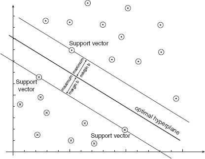
Support vector machine classifiers are inspired by statistical learning theory and they perform structural risk minimization on a nested set structure of separating hyperplanes [10,11]. Viewing the input data as two sets of vectors in a d-dimensional space, an SVM constructs a separating hyperplane in that space, which maximizes the margin between the two classes of points. To compute the margin, two parallel hyperplanes are constructed on each side of the separating one, which are “pushed up against”’ the two classes of points (Fig. 12.1). Intuitively, a good separation is achieved by the hyperplane that has the largest distance to the neighboring datapoints of both classes. A larger margin or distance between these parallel hyperplanes indicates a better generalization error of the classifier. Fundamentally, the SVM classifier is designed for two-class problems. It can be extended to handle multiclass problems by designing a number of one-against-all or one-against-one two-class SVMs.

Suppose a data set consisting of n feature vectors , where , denotes the class label for the datapoint xi. The problem of finding the weight vector w can be formulated as minimizing the following function:

subject to

Here, b is the bias and the function Ф(x) maps the input vector to the feature vector. The dual formulation is given by maximizing the following:

subject to

Only a small fraction of the αi coefficients are nonzero. The corresponding pairs of xi entries are known as support vectors and they fully define the decision function. Geometrically, the support vectors are the points lying near the separating hyperplane. is called the kernel function.

Kernel functions are used for mapping the input space to a higher dimensional feature space so that the classes become linearly separable. Use of four popularly used kernel functions has been studied in this chapter. These are

12.4 PROPOSED TECHNIQUE

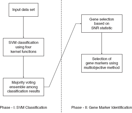
The proposed method consists of two main phases. In the first phase, SVM classifier and ensembling is used for classification purposes. In the subsequent phase, the classification result is used to identify the gene markers.

12.4.1 Phase-I: SVM Classification and Ensemble

From the input preprocessed data set, 50% of the samples are chosen randomly as the training samples. These samples are used to train the four SVM classifiers with four kernel functions mentioned above, respectively. The remaining 50% of the samples are then classified by the four trained classifiers. This process is repeated 50 times resulting in 200 classification solutions. Finally, these solutions are combined through majority voting ensemble to produce a single classification of the samples. The whole process is repeated for 50 data sets created through bootstrapping of samples and genes and the best classification of samples (in terms of classification accuracy) is chosen finally for further processing.

12.4.2 Phase-II: Identification of Gene Markers

Phase two consists of two stages. First, most potential genes are selected based on signal-to-noise ratio (SNR) statistic. Thereafter, a multiobjective genetic algorithm-based feature selection method is employed in order to further reduce the number of selected gene markers.

Stage-I. The final classification result obtained in the previous phase is used to identify the relevant gene markers as follows: Each data set has two classes, one corresponds to normal samples and the other corresponds to malignant samples. For each gene, a statistic called SNR [8] is computed. The SNR is defined as

where μi and σi, i1,2, denote the mean and standard deviation of class i for the corresponding gene. Note that a larger absolute value of SNR for a gene indicates that the gene’s expression level is high in one class and low in another. Hence this bias is very useful in distinguishing the genes that are expressed differently in the two classes of samples.

After computing the SNR statistic for each gene, the genes are sorted in descending order of their SNR values. From the sorted list, the genes whose SNR values are grater than the average SNR value are selected. These genes are mostly responsible for distinguishing the two sample classes.

Stage-II. The set of genes obtained is further reduced by a feature selection technique based on multiobjective genetic algorithm. In this technique, each chromosome is represented as a binary string of length equal to the number of genes selected through the SNR method. The chromosomes encode the information of whether a gene is selected or not. For a chromosome, bit ‘1’ indicates that the corresponding gene is selected, and bit ‘0’ indicates that the corresponding gene is not selected. Here, we have used the nondominated sorting genetic algorithm-II (NSGA-II) [24], a popular multiobjective GA, as the underlying optimization tool. The two objective functions are the classification accuracy and the number of selected genes. The classification accuracy is computed by training a SVM classifier by half of the samples selected randomly, while predicting the class labels of the remaining samples by the trained SVM classifier. The same ensemble technique for combining the four different kernel solutions is used. Note that SVM training and testing is done for the subset of genes encoded in the chromosome. The goal is to maximize the first objective while minimizing the second one simultaneously. The crowded binary tournament selection method as used in [24] followed by conventional uniform crossover and bit-flip mutation operators are used to produce child population from a parent population. From the final nondominated front, the solution with the maximum classification accuracy is selected and the corresponding gene subset is selected as the final set of gene markers.

The different parameters of NSGA-II are selected as follows: number of generations = 100, population size = 50, crossover probability = 0.8, mutation probability = 0.1. All the parameters are set experimentally. Figure 12.2 summarizes the different steps of the two phases.

12.5 DATA SETS AND PREPROCESSING

Three publicly available benchmark cancer data sets, namely, leukemia, colon cancer, and lymphoma data sets have been used for experiments. The data sets and their preprocessing are described in this section.

12.5.1 Leukemia Dataz

The leukemia data set [8] consists of 72 tissue samples. The samples consist of two types of leukemia, 25 of AML and 47 of ALL. The samples are taken from 63 bone marrow samples and 9 peripheral blood samples. There are 7129 genes in the data set. The data set is publicly available at http://www.genome.wi.mit.edu/MPR.

The data set is subjected to a number of preprocessing steps to find out the genes with most variability. The initial gene selection steps followed here are also completely unsupervised. However, more sophisticated methods for gene selection could have been applied. First, we have selected the genes whose expression levels fall between 100 and 15,000. From the resulting 1015 genes, the 100 genes with the largest variation across samples are selected, and the remaining expression values are log-transformed. The resultant data set is of dimension 72× 100.

12.5.2 Colon Cancer Data

The colon cancer data set [7] consists of 62 samples of colon epithelial cells from colon cancer patients. The samples consists of tumor biopsies collected from tumors (40 samples), and normal biopsies collected from healthy parts of the colons (22 samples) of the same patient. The number of genes in the data set is 2000. The data set is publicly available at http://microarray.princeton.edu/oncology.

This data set is preprocessed as follows: First the genes whose expression levels fall between 10 and 15,000 are selected. From the resulting 1756 genes, the 100 genes with the largest variation across samples are selected, and the remaining expression values are log transformed. The resultant data set is of dimension 62× 100.

12.5.3 Lymphoma Data

The diffuse large B-cell lymphoma (DLBCL) data set [6] contains expression measurements of 96 normal and malignant lymphocyte samples each measured using a specialized cDNA microarray, containing 4026 genes that are preferentially expressed in lymphoid cells or which are of known immunological or oncological importance. There are 42 DLBCL and 54 other cancer disease samples. The data set is publicly available at http://genome-www.stanford.edu/lymphoma.

The preprocessing steps for this data set are as follows: As the data set contains some missing values, we have selected only those genes that do not contain any missing value. This results in 854 genes. Thereafter, the top 100 genes with respect to variance are selected. Hence, the data set contains 96 samples, each described by 100 genes.

12.6 EXPERIMENTAL RESULTS

This section first demonstrates the utility of the proposed ensemble classifier method on the three publicly available microarray data sets used for experiments. Thereafter, we have discussed the gene markers identified in the second phase of the proposed technique.

TABLE 12.1 Percentage Classification Accuracy Obtained by Different Kernel Functions and Their Ensemble for All the Data Sets

TABLE 12.2 Number of Gene Markers Selected for Different Data Sets and Performance of Ensemble Classifier on the Set of all 100 Genes and on the Set of Marker Genes in Terms of Classification Accuracy

12.6.1 Classification Results

Table 12.1 reports the percentage classification accuracy obtained by individual kernel functions, as well as by the majority voting ensemble method. It is evident from the table that the ensemble classification provides better classification accuracy compared to that provided by each of the kernel functions. This demonstrates the utility of the proposed ensemble classification technique.

12.6.2 Identification of Gene Markers

Table 12.1 reports the number of gene markers obtained as above for the three data sets. The numbers of gene markers for the three data sets are 11, 8, and 9, respectively. This table also reports the classification accuracy obtained by the proposed ensemble classification technique on the complete preprocessed data sets (with 100 genes) and on the reduced data set consisting of the marker genes only. It is evident from this table that the performance of the proposed technique gets improved when applied to the data set with the identified marker genes only. This indicates the ability of the gene markers to distinguish the two types of samples in all the data sets.

Gene Markers for Leukemia Data In Figure 12.3, the heatmap of the gene versus sample matrix, where the rows correspond to the top 30 genes in terms of SNR statistic scores, and the columns correspond to the ALL and AML samples, is shown. The cells of the heatmap represent the expression levels of the genes in terms of colors. The shades of dark gray represent higher expression level, the shades of light gray represent low expression level, and the colors toward black represent absence of differential expression values. The eleven gene markers identified as discussed are placed at the top 11 rows of the heatmap. It is evident from the figure that these eleven gene markers discriminate the AML samples from the ALL ones. The characteristics of the gene markers are as follows: The genes M92287_at, HG1612-HT1612_at, X51521_at, Z15115_at, U22376_cds2_s_at, X67951_at are upregulated in the ALL samples and downregulated in the AML samples. On the other hand, the genes M63138_at, X62320_at, HG2788-HT2896_at, U46751,_at and L08246_at are downregulated in the ALL samples and upregulated in the AML samples. In Table 12.3, we have reported the eleven gene markers along with their description and associated gene ontological (GO) terms. It is evident from this table that all the eleven genes share most of the GO terms that indicating that these genes have similar molecular functions (mainly related to cell, cell part, and organelle).

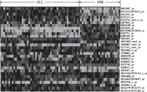
TABLE 12.3 The Description and Associated Gene Ontological (GO) Terms for the Eleven Gene Markers Identified in Leukemia Data

12.6.2.2 Gene Markers for Colon Cancer Data Figure 12.4 shows the heatmap of the gene versus sample matrix for the top 30 gene markers of colon cancer data. The eight gene markers identified as discussed are placed at the top eight rows of the heatmap. It is evident from visual inspection that these eight gene markers partitions the tumor samples from the normal ones. The characteristics of the gene markers are as follows: The genes M63391 and Z24727 are downregulated in the tumor samples and upregulated in the normal samples. On the contrary, the genes T61609, T48804, T57619, M26697, T58861, and T52185 are upregulated in the tumor samples and downregulated in the normal samples. In Table 12.4, the eight gene markers are described along with the associated GO terms. It is evident from this table that all eight genes are mainly take part in metabolic process, cellular process, gene expression, and share most of the GO terms. This indicates that these genes have similar molecular functions.

12.6.2.3 Gene Markers for Lymphoma Data In Figure 12.5, the heatmap for the top 30 gene markers for lymphoma data is shown. The topmost nine gene markers selected using the proposed method are placed at the top nine rows of the heatmap. Visual inspection reveals that these nine gene markers efficiently distinguish the DLBCL samples from the non-DLBCL ones. The characteristics of the gene markers are as follows: The genes 19335, 19338, 20344, 18344, 19368, 20392, and 16770 are upregulated in the non-DLBCL samples and downregulated in the DLBCL samples. On the other hand, the genes 13684 and 16044 are downregulated in the non-DLBCL samples and upregulated in the DLBCL samples. In Table 12.5, we have reported the nine gene markers along with their description and associated GO terms. It is evident from this table that all nine genes share most of the GO terms (mainly related to different kinds of binding functions), indicating that these genes have similar molecular functions.

TABLE 12.4 The Description and Associated GO Terms for the Eight Gene Markers Identified in Colon Cancer Data

TABLE 12.5 The Description and Associated GO Terms for the Nine Gene Markers Identified in Lymphoma Data

12.7 DISCUSSION AND CONCLUSIONS

In this chapter, a cancer classification technique based on support vector machine classifier is proposed. The classification solutions yielded by different classifiers are combined through a majority voting ensemble to obtain the final solution. Further, this classification result is utilized to identify potential gene markers using SNR statistic followed by a multiobjective feature selection technique.

Results on three publicly available benchmark cancer data sets, namely, leukemia, colon cancer and lymphoma, have been demonstrated. The utility of the proposed classification ensemble technique has been demonstrated. The proposed ensemble classifier technique consistently outperformed the other kernel functions considered individually. Finally, relevant gene markers are identified using the classification result. The gene markers identified for different data sets are found to share many GO terms and molecular functions.

As a scope of further research, performance of other popular classifiers and their ensemble is to be studied. Moreover, the gene markers identified are needed to be further investigated biologically.

ACKNOWLEDGMENT

Sanghamitra Bandyopadhyay gratefully acknowledges the financial support received from the grant no. DST/SJF/ET-02/2006-07 under the Swarnajayanti Fellowship scheme of the Department of Science and Technology, Government of India.

REFERENCES

1. S. Bandyopadhyay, A. Mukhopadhyay, and U. Maulik (2007), An improved algorithm for clustering gene expression data, Bioinformatics, 23(21):2859–2865.

2. D. Jiang, C. Tang, and A. Zhang (2004), Cluster analysis for gene expression data: A survey, IEEE Trans. Knowl. Data Eng., 16(11):1370–1386.

3. U. Maulik, A. Mukhopadhyay, and S. Bandyopadhyay (2009), Combining pareto-optimal clusters using supervised learning for identifying co-expressed genes, BMC Bioinformatics, 10(27).

4. W. Shannon, R. Culverhouse, and J. Duncan (2003), Analyzing microarray data using cluster analysis, Pharmacogenomics, 4(1):41–51.

5. R. Shyamsundar, Y. H. Kim, J. P. Higgins, K. Montgomery, M. Jorden, A. Sethuraman, M. van de Rijn, D. Botstein, P. O. Brown, and J. R. Pollack (2005), A DNA microarray survey of gene expression in normal human tissues. Genome Biol., 6:R22.

6. A. A. Alizadeh, M. B. Eisen, R. Davis, C. Ma, I. Lossos, A. Rosenwald, J. Boldrick, R. Warnke, R. Levy, W. Wilson, M. Grever, J. Byrd, D. Botstein, P. O. Brown, and L. M. Straudt (2000), Distinct types of diffuse large b-cell lymphomas identified by gene expression profiling. Nature (London), 403:503–511.

7. U. Alon et al. (1999), Broad patterns of gene expression revealed by clustering analysis of tumor and normal colon tissues probed by oligonucleotide arrays, Proc. Natl. Acad. Sci., USA 96:6745–6750.

8. T. R. Golub, D. K. Slonim, P. Tamayo, C. Huard, M. Gassenbeek, J. P. Mesirov, H. Coller, M. L. Loh, J. R. Downing, M. A. Caligiuri, D. D. Bloomfield, and E. S. Lander (1999), Molecular classification of cancer: class discovery and class prediction by gene expression monitoring, Science, 286:531–537.

9. K. Y. Yeung and R. E. Bumgarner (2003), Multiclass classification of microarray data with repeated measurements: application to cancer, Genome Biol., 4.

10. V. Vapnik (1998), Statistical Learning Theory. John Wiley & Sons, Inc., NY.

11. K. Crammer and Y. Singer (2001), On the algorithmic implementation of multiclass kernel-based vector machines. J. Machine Learning Res., 2:265–292.

12. E. Alba, J. Garcia-Nieto, L. Jourdan, and E-G. Talbi (2007), Gene selection in cancer classification using PSO/SVM and GA/SVM hybrid algorithms. Proceedings of the IEEE Congress Evolution of Computers, IEEE Computer Society, Singapore, pp. 284–290.

13. M. P. S. Brown, W. N. Grundy, D. Lin, N. Cristianini, C. W. Sugnet, T. S. Furey, Jr, and D. Haussler (2000), Knowledge-based analysis of microarray gene expression data by using support vector machines Proc. Natl. Acad. Sci. USA, 97(1):262–267.

14. K. B. Duan, J. C. Rajapakse, H. Wang, and F. Azuaje (2005), Multiple SVM-RFE for gene selection in cancer classification with expression data, IEEE Trans. Nanobiosci., 4(3):228–234.

15. T. S. Furey, N. Cristianini, N. Duffy, D. W. Bednarski, M. Schummer, and D. Haussler (2000), Support vector machine classification and validation of cancer tissue samples using microarray expression data, Bioinformatics, 16(10):906–914.

16. I. Guyon, J. Weston, S. Barnhill, and V. Vapnik (2002), Gene selection for cancer classification using support vector machines, Machine Learning, 46(1-3):389–422.

17. S. Li and M. Tan (2007), Gene selection and tissue classification based on support vector machine and genetic algorithm, Proceedings of the 1st International Conference on Bioformatics and Biomedical Engineering (ICBBE 2007) pp. 192–195.

18. J. Mohr, S. Seo, and K. Obermayer (2008), Automated microarray classification based on P-SVM gene selection. ICMLA ‘08: Proceedings of the 2008 Seventh International Conference on Machine Learning and Applications, IEEE Computer Society, pp. 503–507. Washington, DC.

19. C.A. Coello Coello (2006), Evolutionary multiobjective optimization: A historical view of the field. IEEE Comput. Intell. Mag., 1(1):28–36.

20. C.A. Coello Coello, D.A. Van Veldhuizen, and G.B. Lamont (2006), Evolutionary Algorithms for Solving Multi-Objective Problems, (Genetic and Evolutionary seves) Springer-Verlag, NY.

21. K. Deb ( 2001), Multi-objective Optimization Using Evolutionary Algorithms, John Wiley & Sons, Ltd, England.

22. N. M. Luscombe, D. Greenbaum, and M. Gerstein (2001), What is bioinformatics? A proposed definition and overview of the field. Methods of Information & Medicine, Schatbuer, Vol. 40(4), pp. 346–358.

23. J. Quackenbush (2001), Computational analysis of microarray data, Nat. Rev. Genet., 2:418–427.

24. K. Deb, A. Pratap, S. Agrawal, and T. Meyarivan (2002), A fast and elitist multiobjective genetic algorithm: NSGA-II, IEEE Trans. Evolut. Comput., 6:182–197.