3. Integer Functions
Whole numbers constitute the backbone of discrete mathematics, and we often need to convert from fractions or arbitrary real numbers to integers. Our goal in this chapter is to gain familiarity and fluency with such conversions and to learn some of their remarkable properties.
3.1 Floors and Ceilings
We start by covering the floor (greatest integer) and ceiling (least integer) functions, which are defined for all real x as follows:

Kenneth E. Iverson introduced this notation, as well as the names “floor” and “ceiling,” early in the 1960s [191, page 12]. He found that typesetters could handle the symbols by shaving the tops and bottoms off of ‘[’ and ‘]’. His notation has become sufficiently popular that floor and ceiling brackets can now be used in a technical paper without an explanation of what they mean. Until recently, people had most often been writing ‘[x]’ for the greatest integer ≤ x, without a good equivalent for the least integer function. Some authors had even tried to use ‘]x[’—with a predictable lack of success.
)Ouch.(
Besides variations in notation, there are variations in the functions themselves. For example, some pocket calculators have an INT function, defined as ![]() x
x![]() when x is positive and
when x is positive and ![]() x
x![]() when x is negative. The designers of these calculators probably wanted their INT function to satisfy the identity INT(–x) = –INT(x). But we’ll stick to our floor and ceiling functions, because they have even nicer properties than this.
when x is negative. The designers of these calculators probably wanted their INT function to satisfy the identity INT(–x) = –INT(x). But we’ll stick to our floor and ceiling functions, because they have even nicer properties than this.
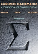
One good way to become familiar with the floor and ceiling functions is to understand their graphs, which form staircase-like patterns above and below the line f(x) = x:
We see from the graph that, for example,
![]() e
e![]() = 2,
= 2, ![]() –e
–e![]() = –3,
= –3,
![]() e
e![]() = 3,
= 3, ![]() –e
–e![]() = –2,
= –2,
since e = 2.71828 . . . .
By staring at this illustration we can observe several facts about floors and ceilings. First, since the floor function lies on or below the diagonal line f(x) = x, we have ![]() x
x![]() ≤ x; similarly
≤ x; similarly ![]() x
x![]() ≥ x. (This, of course, is quite obvious from the definition.) The two functions are equal precisely at the integer points:
≥ x. (This, of course, is quite obvious from the definition.) The two functions are equal precisely at the integer points:
![]() x
x![]() = x
= x ![]() x is an integer
x is an integer ![]()
![]() x
x![]() = x .
= x .
(We use the notation ‘⇔’ to mean “if and only if.”) Furthermore, when they differ the ceiling is exactly 1 higher than the floor:
Cute.
By Iverson’s bracket convention, this is a complete equation.
If we shift the diagonal line down one unit, it lies completely below the floor function, so x – 1 < ![]() x
x![]() ; similarly x + 1 >
; similarly x + 1 > ![]() x
x![]() . Combining these observations gives us
. Combining these observations gives us
Finally, the functions are reflections of each other about both axes:
Thus each is easily expressible in terms of the other. This fact helps to explain why the ceiling function once had no notation of its own. But we see ceilings often enough to warrant giving them special symbols, just as we have adopted special notations for rising powers as well as falling powers. Mathematicians have long had both sine and cosine, tangent and cotangent, secant and cosecant, max and min; now we also have both floor and ceiling.
Next week we’re getting walls.
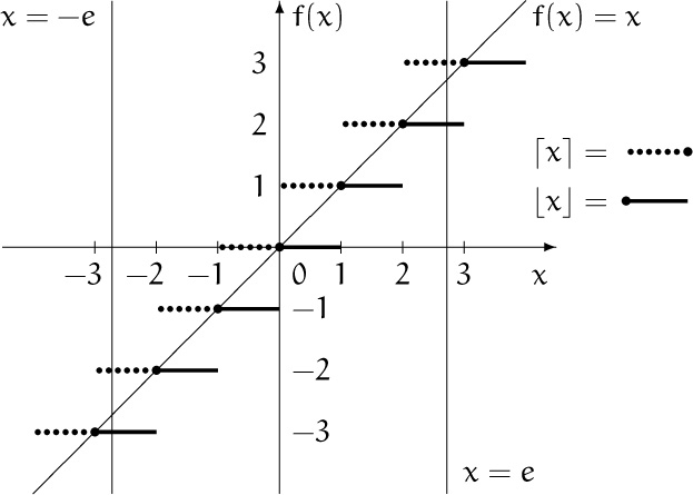
To actually prove properties about the floor and ceiling functions, rather than just to observe such facts graphically, the following four rules are especially useful:
(We assume in all four cases that n is an integer and that x is real.) Rules (a) and (c) are immediate consequences of definition (3.1); rules (b) and (d) are the same but with the inequalities rearranged so that n is in the middle.
It’s possible to move an integer term in or out of a floor (or ceiling):
(Because rule (3.5(a)) says that this assertion is equivalent to the inequalities ![]() x
x![]() + n ≤ x + n <
+ n ≤ x + n < ![]() x
x![]() + n + 1.) But similar operations, like moving out a constant factor, cannot be done in general. For example, we have
+ n + 1.) But similar operations, like moving out a constant factor, cannot be done in general. For example, we have ![]() nx
nx![]() ≠ n
≠ n![]() x
x![]() when n = 2 and x = 1/2. This means that floor and ceiling brackets are comparatively inflexible. We are usually happy if we can get rid of them or if we can prove anything at all when they are present.
when n = 2 and x = 1/2. This means that floor and ceiling brackets are comparatively inflexible. We are usually happy if we can get rid of them or if we can prove anything at all when they are present.
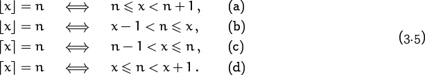
It turns out that there are many situations in which floor and ceiling brackets are redundant, so that we can insert or delete them at will. For example, any inequality between a real and an integer is equivalent to a floor or ceiling inequality between integers:
These rules are easily proved. For example, if x < n then surely ![]() x
x![]() < n, since
< n, since ![]() x
x![]() ≤ x. Conversely, if
≤ x. Conversely, if ![]() x
x![]() < n then we must have x < n, since x <
< n then we must have x < n, since x < ![]() x
x![]() + 1 and
+ 1 and ![]() x
x![]() + 1 ≤ n.
+ 1 ≤ n.
It would be nice if the four rules in (3.7) were as easy to remember as they are to prove. Each inequality without floor or ceiling corresponds to the same inequality with floor or with ceiling; but we need to think twice before deciding which of the two is appropriate.
The difference between x and ![]() x
x![]() is called the fractional part of x, and it arises often enough in applications to deserve its own notation:
is called the fractional part of x, and it arises often enough in applications to deserve its own notation:
Hmmm. We’d better not write {x} for the fractional part when it could be confused with the set containing x as its only element.
We sometimes call ![]() x
x![]() the integer part of x, since x =
the integer part of x, since x = ![]() x
x![]() + {x}. If a real number x can be written in the form x = n + θ, where n is an integer and 0 ≤ θ < 1, we can conclude by (3.5(a)) that n =
+ {x}. If a real number x can be written in the form x = n + θ, where n is an integer and 0 ≤ θ < 1, we can conclude by (3.5(a)) that n = ![]() x
x![]() and θ = {x}.
and θ = {x}.
Identity (3.6) doesn’t hold if n is an arbitrary real. But we can deduce that there are only two possibilities for ![]() x + y
x + y![]() in general: If we write x =
in general: If we write x = ![]() x
x![]() + {x} and y =
+ {x} and y = ![]() y
y![]() + {y}, then we have
+ {y}, then we have ![]() x + y
x + y![]() =
= ![]() x
x![]() +
+ ![]() y
y![]() +
+ ![]() {x} + {y}
{x} + {y}![]() . And since 0 ≤ {x} + {y} < 2, we find that sometimes
. And since 0 ≤ {x} + {y} < 2, we find that sometimes ![]() x + y
x + y![]() is
is ![]() x
x![]() +
+ ![]() y
y![]() , otherwise it’s
, otherwise it’s ![]() x
x![]() +
+ ![]() y
y![]() + 1.
+ 1.
The second case occurs if and only if there’s a “carry” at the position of the decimal point, when the fractional parts {x} and {y} are added together.
3.2 Floor/Ceiling Applications
We’ve now seen the basic tools for handling floors and ceilings. Let’s put them to use, starting with an easy problem: What’s ![]() lg 35
lg 35![]() ? (Following a convention that many authors have proposed independently, we use ‘lg’ to denote the base-2 logarithm.) Well, since 25 < 35 ≤ 26, we can take logs to get 5 < lg 35 ≤ 6; so relation (3.5(c)) tells us that
? (Following a convention that many authors have proposed independently, we use ‘lg’ to denote the base-2 logarithm.) Well, since 25 < 35 ≤ 26, we can take logs to get 5 < lg 35 ≤ 6; so relation (3.5(c)) tells us that ![]() lg 35
lg 35![]() = 6.
= 6.
Note that the number 35 is six bits long when written in radix 2 notation: 35 = (100011)2. Is it always true that ![]() lg n
lg n![]() is the length of n written in binary? Not quite. We also need six bits to write 32 = (100000)2. So
is the length of n written in binary? Not quite. We also need six bits to write 32 = (100000)2. So ![]() lg n
lg n![]() is the wrong answer to the problem. (It fails only when n is a power of 2, but that’s infinitely many failures.) We can find a correct answer by realizing that it takes m bits to write each number n such that 2m–1 ≤ n < 2m; thus (3.5(a)) tells us that m – 1 =
is the wrong answer to the problem. (It fails only when n is a power of 2, but that’s infinitely many failures.) We can find a correct answer by realizing that it takes m bits to write each number n such that 2m–1 ≤ n < 2m; thus (3.5(a)) tells us that m – 1 = ![]() lg n
lg n![]() , so m =
, so m = ![]() lg n
lg n![]() + 1. That is, we need
+ 1. That is, we need ![]() lg n
lg n![]() + 1 bits to express n in binary, for all n > 0. Alternatively, a similar derivation yields the answer
+ 1 bits to express n in binary, for all n > 0. Alternatively, a similar derivation yields the answer ![]() lg(n + 1)
lg(n + 1)![]() ; this formula holds for n = 0 as well, if we’re willing to say that it takes zero bits to write n = 0 in binary.
; this formula holds for n = 0 as well, if we’re willing to say that it takes zero bits to write n = 0 in binary.
Let’s look next at expressions with several floors or ceilings. What is ![]()
![]() x
x![]()
![]() ? Easy—since
? Easy—since ![]() x
x![]() is an integer,
is an integer, ![]()
![]() x
x![]()
![]() is just
is just ![]() x
x![]() . So is any other expression with an innermost
. So is any other expression with an innermost ![]() x
x![]() surrounded by any number of floors or ceilings.
surrounded by any number of floors or ceilings.
Here’s a tougher problem: Prove or disprove the assertion
(Of course π, e, and ϕ are the obvious first real numbers to try, aren’t they?)
Equality obviously holds when x is an integer, because x = ![]() x
x![]() . And there’s equality in the special cases π = 3.14159 . . . , e = 2.71828 . . . , and
. And there’s equality in the special cases π = 3.14159 . . . , e = 2.71828 . . . , and ![]() , because we get 1 = 1. Our failure to find a counterexample suggests that equality holds in general, so let’s try to prove it.
, because we get 1 = 1. Our failure to find a counterexample suggests that equality holds in general, so let’s try to prove it.
Incidentally, when we’re faced with a “prove or disprove,” we’re usually better off trying first to disprove with a counterexample, for two reasons: A disproof is potentially easier (we need just one counterexample); and nit-picking arouses our creative juices. Even if the given assertion is true, our search for a counterexample often leads us to a proof, as soon as we see why a counterexample is impossible. Besides, it’s healthy to be skeptical.
Skepticism is healthy only to a limited extent. Being skeptical about proofs and programs (particularly your own) will probably keep your grades healthy and your job fairly secure. But applying that much skepticism will probably also keep you shut away working all the time, instead of letting you get out for exercise and relaxation.
Too much skepticism is an open invitation to the state of rigor mortis, where you become so worried about being correct and rigorous that you never get anything finished.
—A skeptic
If we try to prove that ![]() with the help of calculus, we might start by decomposing x into its integer and fractional parts
with the help of calculus, we might start by decomposing x into its integer and fractional parts ![]() x
x![]() + {x} = n + θ and then expanding the square root using the binomial theorem: (n+θ)1/2 = n1/2 + n–1/2θ/2 – n–3/2θ2/8 + · · · . But this approach gets pretty messy.
+ {x} = n + θ and then expanding the square root using the binomial theorem: (n+θ)1/2 = n1/2 + n–1/2θ/2 – n–3/2θ2/8 + · · · . But this approach gets pretty messy.
It’s much easier to use the tools we’ve developed. Here’s a possible strategy: Somehow strip off the outer floor and square root of ![]() , then remove the inner floor, then add back the outer stuff to get
, then remove the inner floor, then add back the outer stuff to get ![]() . OK. We let
. OK. We let ![]() and invoke (3.5(a)), giving
and invoke (3.5(a)), giving ![]() . That removes the outer floor bracket without losing any information. Squaring, since all three expressions are nonnegative, we have m2 ≤
. That removes the outer floor bracket without losing any information. Squaring, since all three expressions are nonnegative, we have m2 ≤ ![]() x
x![]() < (m + 1)2. That gets rid of the square root. Next we remove the floor, using (3.7(d)) for the left inequality and (3.7(a)) for the right: m2 ≤ x < (m + 1)2. It’s now a simple matter to retrace our steps, taking square roots to get
< (m + 1)2. That gets rid of the square root. Next we remove the floor, using (3.7(d)) for the left inequality and (3.7(a)) for the right: m2 ≤ x < (m + 1)2. It’s now a simple matter to retrace our steps, taking square roots to get ![]() and invoking (3.5(a)) to get
and invoking (3.5(a)) to get ![]() . Thus
. Thus ![]() ; the assertion is true. Similarly, we can prove that
; the assertion is true. Similarly, we can prove that
The proof we just found doesn’t rely heavily on the properties of square roots. A closer look shows that we can generalize the ideas and prove much more: Let f(x) be any continuous, monotonically increasing function on an interval of the real numbers, with the property that
f(x) = integer ![]() x = integer.
x = integer.
(The symbol ‘⇒’ means “implies.”) Then we have
(This observation was made by R. J. McEliece when he was an undergrad.)
whenever f(x), f(![]() x
x![]() ), and f(
), and f(![]() x
x![]() ) are defined. Let’s prove this general property for ceilings, since we did floors earlier and since the proof for floors is almost the same. If x =
) are defined. Let’s prove this general property for ceilings, since we did floors earlier and since the proof for floors is almost the same. If x = ![]() x
x![]() , there’s nothing to prove. Otherwise x <
, there’s nothing to prove. Otherwise x < ![]() x
x![]() , and f(x) < f(
, and f(x) < f(![]() x
x![]() ) since f is increasing. Hence
) since f is increasing. Hence ![]() f(x)
f(x)![]() ≤
≤ ![]() f(
f(![]() x
x![]() )
)![]() , since
, since ![]()
![]() is nondecreasing. If
is nondecreasing. If ![]() f(x)
f(x)![]() <
< ![]() f(
f(![]() x
x![]() )
)![]() , there must be a number y such that x ≤ y <
, there must be a number y such that x ≤ y < ![]() x
x![]() and f(y) =
and f(y) = ![]() f(x)
f(x)![]() , since f is continuous. This y is an integer, because of f’s special property. But there cannot be an integer strictly between
, since f is continuous. This y is an integer, because of f’s special property. But there cannot be an integer strictly between ![]() x
x![]() and
and ![]() x
x![]() . This contradiction implies that we must have
. This contradiction implies that we must have ![]() f(x)
f(x)![]() =
= ![]() f(
f(![]() x
x![]() )
)![]() .
.
An important special case of this theorem is worth noting explicitly:
if m and n are integers and the denominator n is positive. For example, let m = 0; we have ![]()
![]()
![]() x/10
x/10![]() /10
/10![]() /10
/10![]() =
= ![]() x/1000
x/1000![]() . Dividing thrice by 10 and throwing off digits is the same as dividing by 1000 and tossing the remainder.
. Dividing thrice by 10 and throwing off digits is the same as dividing by 1000 and tossing the remainder.
Let’s try now to prove or disprove another statement:
This works when x = π and x = e, but it fails when x = ϕ; so we know that it isn’t true in general.
Before going any further, let’s digress a minute to discuss different levels of problems that might appear in books about mathematics:
Level 1. Given an explicit object x and an explicit property P(x), prove that P(x) is true. For example, “Prove that ![]() π
π![]() = 3.” Here the problem involves finding a proof of some purported fact.
= 3.” Here the problem involves finding a proof of some purported fact.
Level 2. Given an explicit set X and an explicit property P(x), prove that P(x) is true for all x ![]() X. For example, “Prove that
X. For example, “Prove that ![]() x
x![]() ≤ x for all real x.” Again the problem involves finding a proof, but the proof this time must be general. We’re doing algebra, not just arithmetic.
≤ x for all real x.” Again the problem involves finding a proof, but the proof this time must be general. We’re doing algebra, not just arithmetic.
Level 3. Given an explicit set X and an explicit property P(x), prove or disprove that P(x) is true for all x ![]() X. For example, “Prove or disprove that
X. For example, “Prove or disprove that ![]() for all real x ≥ 0.” Here there’s an additional level of uncertainty; the outcome might go either way. This is closer to the real situation a mathematician constantly faces: Assertions that get into books tend to be true, but new things have to be looked at with a jaundiced eye. If the statement is false, our job is to find a counterexample. If the statement is true, we must find a proof as in level 2.
for all real x ≥ 0.” Here there’s an additional level of uncertainty; the outcome might go either way. This is closer to the real situation a mathematician constantly faces: Assertions that get into books tend to be true, but new things have to be looked at with a jaundiced eye. If the statement is false, our job is to find a counterexample. If the statement is true, we must find a proof as in level 2.
In my other texts “prove or disprove” seems to mean the same as “prove,” about 99.44% of the time; but not in this book.
Level 4. Given an explicit set X and an explicit property P(x), find a necessary and sufficient condition Q(x) that P(x) is true. For example, “Find a necessary and sufficient condition that ![]() x
x![]() ≥
≥ ![]() x
x![]() .” The problem is to find Q such that P(x) ⇔ Q(x). Of course, there’s always a trivial answer; we can take Q(x) = P(x). But the implied requirement is to find a condition that’s as simple as possible. Creativity is required to discover a simple condition that will work. (For example, in this case, “
.” The problem is to find Q such that P(x) ⇔ Q(x). Of course, there’s always a trivial answer; we can take Q(x) = P(x). But the implied requirement is to find a condition that’s as simple as possible. Creativity is required to discover a simple condition that will work. (For example, in this case, “![]() x
x![]() ≥
≥ ![]() x
x![]() ⇔ x is an integer.”) The extra element of discovery needed to find Q(x) makes this sort of problem more difficult, but it’s more typical of what mathematicians must do in the “real world.” Finally, of course, a proof must be given that P(x) is true if and only if Q(x) is true.
⇔ x is an integer.”) The extra element of discovery needed to find Q(x) makes this sort of problem more difficult, but it’s more typical of what mathematicians must do in the “real world.” Finally, of course, a proof must be given that P(x) is true if and only if Q(x) is true.
But no simpler.
—A. Einstein
Level 5. Given an explicit set X, find an interesting property P(x) of its elements. Now we’re in the scary domain of pure research, where students might think that total chaos reigns. This is real mathematics. Authors of textbooks rarely dare to pose level 5 problems.
End of digression. But let’s convert the last question we looked at from level 3 to level 4: What is a necessary and sufficient condition that ![]() We have observed that equality holds when x = 3.142 but not when x = 1.618; further experimentation shows that it fails also when x is between 9 and 10. Oho. Yes. We see that bad cases occur whenever m2 < x < m2 + 1, since this gives m on the left and m + 1 on the right. In all other cases where
We have observed that equality holds when x = 3.142 but not when x = 1.618; further experimentation shows that it fails also when x is between 9 and 10. Oho. Yes. We see that bad cases occur whenever m2 < x < m2 + 1, since this gives m on the left and m + 1 on the right. In all other cases where ![]() is defined, namely when x = 0 or m2 + 1 ≤ x ≤ (m + 1)2, we get equality. The following statement is therefore necessary and sufficient for equality: Either x is an integer or
is defined, namely when x = 0 or m2 + 1 ≤ x ≤ (m + 1)2, we get equality. The following statement is therefore necessary and sufficient for equality: Either x is an integer or ![]() isn’t.
isn’t.
Home of the Toledo Mudhens.
For our next problem let’s consider a handy new notation, suggested by C. A. R. Hoare and Lyle Ramshaw, for intervals of the real line: [α . . β] denotes the set of real numbers x such that α ≤ x ≤ β. This set is called a closed interval because it contains both endpoints α and β. The interval containing neither endpoint, denoted by (α . . β), consists of all x such that α < x < β; this is called an open interval. And the intervals [α . . β) and (α . . β], which contain just one endpoint, are defined similarly and called half-open.
(Or, by pessimists, half-closed.)
How many integers are contained in such intervals? The half-open intervals are easier, so we start with them. In fact half-open intervals are almost always nicer than open or closed intervals. For example, they’re additive—we can combine the half-open intervals [α . . β) and [β . . γ) to form the half-open interval [α . . γ). This wouldn’t work with open intervals because the point β would be excluded, and it could cause problems with closed intervals because β would be included twice.
Back to our problem. The answer is easy if α and β are integers: Then [α . . β) contains the β – α integers α, α + 1, . . . , β – 1, assuming that α ≤ β. Similarly (α . . β] contains β – α integers in such a case. But our problem is harder, because α and β are arbitrary reals. We can convert it to the easier problem, though, since
α ≤ n < β ![]()
![]() α
α![]() ≤ n <
≤ n < ![]() β
β![]() ,
,
α < n ≤ β ![]()
![]() α
α![]() < n ≤
< n ≤ ![]() β
β![]() ,
,
when n is an integer, according to (3.7). The intervals on the right have integer endpoints and contain the same number of integers as those on the left, which have real endpoints. So the interval [α . . β) contains exactly ![]() β
β![]() –
– ![]() α
α![]() integers, and (α . . β] contains
integers, and (α . . β] contains ![]() β
β![]() –
– ![]() α
α![]() . This is a case where we actually want to introduce floor or ceiling brackets, instead of getting rid of them.
. This is a case where we actually want to introduce floor or ceiling brackets, instead of getting rid of them.
By the way, there’s a mnemonic for remembering which case uses floors and which uses ceilings: Half-open intervals that include the left endpoint but not the right (such as 0 ≤ θ < 1) are slightly more common than those that include the right endpoint but not the left; and floors are slightly more common than ceilings. So by Murphy’s Law, the correct rule is the opposite of what we’d expect—ceilings for [α . . β) and floors for (α . . β].
Just like we can remember the date of Columbus’s departure by singing, “In fourteen hundred and ninety-three/Columbus sailed the deep blue sea.”
Similar analyses show that the closed interval [α . . β] contains exactly ![]() β
β![]() –
–![]() α
α![]() +1 integers and that the open interval (α . . β) contains
+1 integers and that the open interval (α . . β) contains ![]() β
β![]() –
–![]() α
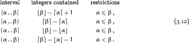
α![]() –1; but we place the additional restriction α ≠ β on the latter so that the formula won’t ever embarrass us by claiming that an empty interval (α . . α) contains a total of –1 integers. To summarize, we’ve deduced the following facts:
–1; but we place the additional restriction α ≠ β on the latter so that the formula won’t ever embarrass us by claiming that an empty interval (α . . α) contains a total of –1 integers. To summarize, we’ve deduced the following facts:
Now here’s a problem we can’t refuse. The Concrete Math Club has a casino (open only to purchasers of this book) in which there’s a roulette wheel with one thousand slots, numbered 1 to 1000. If the number n that comes up on a spin is divisible by the floor of its cube root, that is, if
then it’s a winner and the house pays us $5; otherwise it’s a loser and we must pay $1. (The notation ab, read “a divides b,” means that b is an exact multiple of a; Chapter 4 investigates this relation carefully.) Can we expect to make money if we play this game?
We can compute the average winnings—that is, the amount we’ll win (or lose) per play—by first counting the number W of winners and the number L = 1000 – W of losers. If each number comes up once during 1000 plays, we win 5W dollars and lose L dollars, so the average winnings will be
(A poll of the class at this point showed that 28 students thought it was a bad idea to play, 13 wanted to gamble, and the rest were too confused to answer.)
(So we hit them with the Concrete Math Club.)
If there are 167 or more winners, we have the advantage; otherwise the advantage is with the house.
How can we count the number of winners among 1 through 1000? It’s not hard to spot a pattern. The numbers from 1 through 23 – 1 = 7 are all winners because ![]() for each. Among the numbers 23 = 8 through 33 – 1 = 26, only the even numbers are winners. And among 33 = 27 through 43 – 1 = 63, only those divisible by 3 are. And so on.
for each. Among the numbers 23 = 8 through 33 – 1 = 26, only the even numbers are winners. And among 33 = 27 through 43 – 1 = 63, only those divisible by 3 are. And so on.
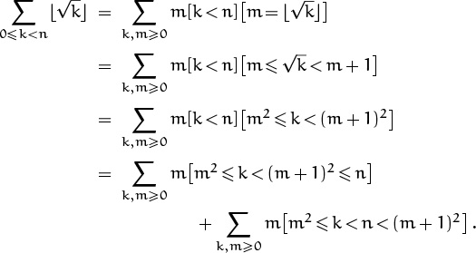
The whole setup can be analyzed systematically if we use the summation techniques of Chapter 2, taking advantage of Iverson’s convention about logical statements evaluating to 0 or 1:
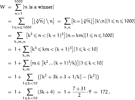
This derivation merits careful study. Notice that line 6 uses our formula (3.12) for the number of integers in a half-open interval. The only “difficult” maneuver is the decision made between lines 3 and 4 to treat n = 1000 as a special case. (The inequality k3 ≤ n < (k + 1)3 does not combine easily with 1 ≤ n ≤ 1000 when k = 10.) In general, boundary conditions tend to be the most critical part of ∑-manipulations.
True.
Where did you say this casino is?
The bottom line says that W = 172; hence our formula for average winnings per play reduces to (6·172 – 1000)/1000 dollars, which is 3.2 cents. We can expect to be about $3.20 richer after making 100 bets of $1 each. (Of course, the house may have made some numbers more equal than others.)
The casino problem we just solved is a dressed-up version of the more mundane question, “How many integers n, where 1 ≤ n ≤ 1000, satisfy the relation ![]() ” Mathematically the two questions are the same. But sometimes it’s a good idea to dress up a problem. We get to use more vocabulary (like “winners” and “losers”), which helps us to understand what’s going on.
” Mathematically the two questions are the same. But sometimes it’s a good idea to dress up a problem. We get to use more vocabulary (like “winners” and “losers”), which helps us to understand what’s going on.
Let’s get general. Suppose we change 1000 to 1000000, or to an even larger number, N. (We assume that the casino has connections and can get a bigger wheel.) Now how many winners are there?
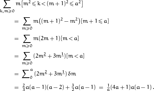
The same argument applies, but we need to deal more carefully with the largest value of k, which we can call K for convenience:
(Previously K was 10.) The total number of winners for general N comes to

We know that the remaining sum is ![]() N/K
N/K![]() –
– ![]() K2
K2![]() + 1 =
+ 1 = ![]() N/K
N/K![]() – K2 + 1; hence the formula
– K2 + 1; hence the formula
gives the general answer for a wheel of size N.
The first two terms of this formula are approximately ![]() , and the other terms are much smaller in comparison, when N is large. In Chapter 9 we’ll learn how to derive expressions like
, and the other terms are much smaller in comparison, when N is large. In Chapter 9 we’ll learn how to derive expressions like
W = ![]() N2/3 + O(N1/3),
N2/3 + O(N1/3),
where O(N1/3) stands for a quantity that is no more than a constant times N1/3. Whatever the constant is, we know that it’s independent of N; so for large N the contribution of the O-term to W will be quite small compared with ![]() . For example, the following table shows how close
. For example, the following table shows how close ![]() is to W:
is to W:

It’s a pretty good approximation.
Approximate formulas are useful because they’re simpler than formulas with floors and ceilings. However, the exact truth is often important, too, especially for the smaller values of N that tend to occur in practice. For example, the casino owner may have falsely assumed that there are only ![]() winners when N = 1000 (in which case there would be a 10¢ advantage for the house).
winners when N = 1000 (in which case there would be a 10¢ advantage for the house).
Our last application in this section looks at so-called spectra. We define the spectrum of a positive real number α to be an infinite multiset of integers,
Spec(α) = {![]() α
α![]() ,
, ![]() 2α
2α![]() ,
, ![]() 3α
3α![]() , . . . } .
, . . . } .
(A multiset is like a set but it can have repeated elements.) For example, the spectrum of 1/2 starts out {0, 1, 1, 2, 2, 3, 3, . . . }.
It’s easy to prove that no two spectra are equal—that α ≠ β implies Spec(α) ≠ Spec(β). For, assuming without loss of generality that α < β, there’s a positive integer m such that m(β – α) ≥ 1. (In fact, any m ≥ ![]() 1/(β – α)
1/(β – α)![]() will do; but we needn’t show off our knowledge of floors and ceilings all the time.) Hence mβ – mα ≥ 1, and
will do; but we needn’t show off our knowledge of floors and ceilings all the time.) Hence mβ – mα ≥ 1, and ![]() mβ
mβ![]() >
> ![]() mα
mα![]() . Thus Spec(β) has fewer than m elements ≤
. Thus Spec(β) has fewer than m elements ≤ ![]() mα
mα![]() , while Spec(α) has at least m.
, while Spec(α) has at least m.
. . . without lots of generality . . .
Spectra have many beautiful properties. For example, consider the two multisets

“If x be an incommensurable number less than unity, one of the series of quantities m/x, m/(1 – x), where m is a whole number, can be found which shall lie between any given consecutive integers, and but one such quantity can be found.”
—Rayleigh [304]
It’s easy to calculate Spec(![]() ) with a pocket calculator, and the nth element of Spec(
) with a pocket calculator, and the nth element of Spec(![]() ) is just 2n more than the nth element of Spec(
) is just 2n more than the nth element of Spec(![]() ), by (3.6). A closer look shows that these two spectra are also related in a much more surprising way: It seems that any number missing from one is in the other, but that no number is in both! And it’s true: The positive integers are the disjoint union of Spec(
), by (3.6). A closer look shows that these two spectra are also related in a much more surprising way: It seems that any number missing from one is in the other, but that no number is in both! And it’s true: The positive integers are the disjoint union of Spec(![]() ) and Spec(
) and Spec(![]() ). We say that these spectra form a partition of the positive integers.
). We say that these spectra form a partition of the positive integers.
Right, because exactly one of the counts must increase when n increases by 1.
To prove this assertion, we will count how many of the elements of Spec(![]() ) are ≤ n, and how many of the elements of Spec(
) are ≤ n, and how many of the elements of Spec(![]() ) are ≤ n. If the total is n, for each n, these two spectra do indeed form a partition.
) are ≤ n. If the total is n, for each n, these two spectra do indeed form a partition.
Whenever α > 0, the number of elements in Spec(α) that are ≤ n is
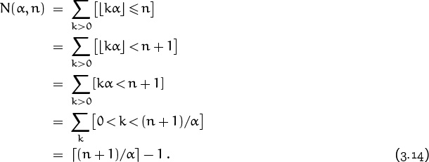
This derivation has two special points of interest. First, it uses the law
to change ‘≤’ to ‘<’, so that the floor brackets can be removed by (3.7). Also—and this is more subtle—it sums over the range k > 0 instead of k ≥ 1, because (n + 1)/α might be less than 1 for certain n and α. If we had tried to apply (3.12) to determine the number of integers in [1 . . (n + 1)/α), rather than the number of integers in (0 . . (n+1)/α), we would have gotten the right answer; but our derivation would have been faulty because the conditions of applicability wouldn’t have been met.
Good, we have a formula for N(α, n). Now we can test whether or not Spec(![]() ) and Spec(
) and Spec(![]() ) partition the positive integers, by testing whether or not
) partition the positive integers, by testing whether or not ![]() for all integers n > 0, using (3.14):
for all integers n > 0, using (3.14):
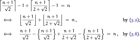
Everything simplifies now because of the neat identity
our condition reduces to testing whether or not
for all n > 0. And we win, because these are the fractional parts of two noninteger numbers that add up to the integer n + 1. A partition it is.
3.3 Floor/Ceiling Recurrences
Floors and ceilings add an interesting new dimension to the study of recurrence relations. Let’s look first at the recurrence

Thus, for example, K1 is 1 + min(2K0, 3K0) = 3; the sequence begins 1, 3, 3, 4, 7, 7, 7, 9, 9, 10, 13, . . . . One of the authors of this book has modestly decided to call these the Knuth numbers.
Exercise 25 asks for a proof or disproof that Kn ≥ n, for all n ≥ 0. The first few K’s just listed do satisfy the inequality, so there’s a good chance that it’s true in general. Let’s try an induction proof: The basis n = 0 comes directly from the defining recurrence. For the induction step, we assume that the inequality holds for all values up through some fixed nonnegative n, and we try to show that Kn+1 ≥ n + 1. From the recurrence we know that Kn+1 = 1 + min(2K![]() n/2
n/2![]() , 3K
, 3K![]() n/3
n/3![]() ). The induction hypothesis tells us that 2K
). The induction hypothesis tells us that 2K![]() n/2
n/2![]() ≥ 2
≥ 2![]() n/2
n/2![]() and 3K
and 3K![]() n/3
n/3![]() ≥ 3
≥ 3![]() n/3
n/3![]() . However, 2
. However, 2![]() n/2
n/2![]() can be as small as n – 1, and 3
can be as small as n – 1, and 3![]() n/3
n/3![]() can be as small as n – 2. The most we can conclude from our induction hypothesis is that Kn+1 ≥ 1 + (n – 2); this falls far short of Kn+1 ≥ n + 1.
can be as small as n – 2. The most we can conclude from our induction hypothesis is that Kn+1 ≥ 1 + (n – 2); this falls far short of Kn+1 ≥ n + 1.
We now have reason to worry about the truth of Kn ≥ n, so let’s try to disprove it. If we can find an n such that either 2K![]() n/2
n/2![]() < n or 3K
< n or 3K![]() n/3
n/3![]() < n, or in other words such that
< n, or in other words such that
K![]() n/2
n/2![]() < n/2 or K
< n/2 or K![]() n/3
n/3![]() < n/3,
< n/3,
we will have Kn+1 < n + 1. Can this be possible? We’d better not give the answer away here, because that will spoil exercise 25.
Recurrence relations involving floors and/or ceilings arise often in computer science, because algorithms based on the important technique of “divide and conquer” often reduce a problem of size n to the solution of similar problems of integer sizes that are fractions of n. For example, one way to sort n records, if n > 1, is to divide them into two approximately equal parts, one of size ![]() n/2
n/2![]() and the other of size
and the other of size ![]() n/2
n/2![]() . (Notice, incidentally, that
. (Notice, incidentally, that
this formula comes in handy rather often.) After each part has been sorted separately (by the same method, applied recursively), we can merge the records into their final order by doing at most n – 1 further comparisons. Therefore the total number of comparisons performed is at most f(n), where
A solution to this recurrence appears in exercise 34.
The Josephus problem of Chapter 1 has a similar recurrence, which can be cast in the form
J(1) = 1;
J(n) = 2J(![]() n/2
n/2![]() ) – (–1)n, for n > 1.
) – (–1)n, for n > 1.
We’ve got more tools to work with than we had in Chapter 1, so let’s consider the more authentic Josephus problem in which every third person is eliminated, instead of every second. If we apply the methods that worked in Chapter 1 to this more difficult problem, we wind up with a recurrence like
where ‘mod’ is a function that we will be studying shortly, and where we have an = –2, +1, or ![]() according as n mod 3 = 0, 1, or 2. But this recurrence is too horrible to pursue.
according as n mod 3 = 0, 1, or 2. But this recurrence is too horrible to pursue.
There’s another approach to the Josephus problem that gives a much better setup. Whenever a person is passed over, we can assign a new number. Thus, 1 and 2 become n + 1 and n + 2, then 3 is executed; 4 and 5 become n + 3 and n + 4, then 6 is executed; . . . ; 3k + 1 and 3k + 2 become n + 2k + 1 and n + 2k + 2, then 3k + 3 is executed; . . . then 3n is executed (or left to survive). For example, when n = 10 the numbers are
The kth person eliminated ends up with number 3k. So we can figure out who the survivor is if we can figure out the original number of person number 3n.
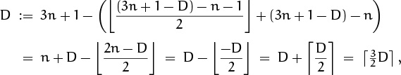
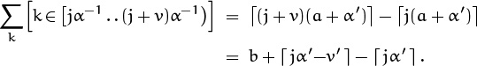
If N > n, person number N must have had a previous number, and we can find it as follows: We have N = n + 2k + 1 or N = n + 2k + 2, hence k = ![]() (N – n – 1)/2
(N – n – 1)/2![]() ; the previous number was 3k + 1 or 3k + 2, respectively. That is, it was 3k + (N – n – 2k) = k + N – n. Hence we can calculate the survivor’s number J3(n) as follows:
; the previous number was 3k + 1 or 3k + 2, respectively. That is, it was 3k + (N – n – 2k) = k + N – n. Hence we can calculate the survivor’s number J3(n) as follows:

“Not too slow, not too fast.”
—L. Armstrong
This is not a closed form for J3(n); it’s not even a recurrence. But at least it tells us how to calculate the answer reasonably fast, if n is large.
Fortunately there’s a way to simplify this algorithm if we use the variable D = 3n + 1 – N in place of N. (This change in notation corresponds to assigning numbers from 3n down to 1, instead of from 1 up to 3n; it’s sort of like a countdown.) Then the complicated assignment to N becomes
and we can rewrite the algorithm as follows:
D := 1;
while D ≤ 2n do D := ![]()
![]() D
D![]() ;
;
J3(n) := 3n + 1 – D .
Aha! This looks much nicer, because n enters the calculation in a very simple way. In fact, we can show by the same reasoning that the survivor Jq(n) when every qth person is eliminated can be calculated as follows:
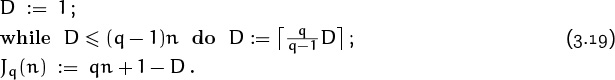
In the case q = 2 that we know so well, this makes D grow to 2m+1 when n = 2m + l; hence J2(n) = 2(2m + l) + 1 – 2m+1 = 2l + 1. Good.
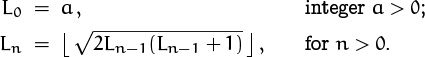
The recipe in (3.19) computes a sequence of integers that can be defined by the following recurrence:

“Known” like, say, harmonic numbers. A. M. Odlyzko and H. S. Wilf have shown [283] that ![]() , where C ≈ 1.622270503.
, where C ≈ 1.622270503.
These numbers don’t seem to relate to any familiar functions in a simple way, except when q = 2; hence they probably don’t have a nice closed form. But if we’re willing to accept the sequence ![]() as “known,” then it’s easy to describe the solution to the generalized Josephus problem: The survivor Jq(n) is
as “known,” then it’s easy to describe the solution to the generalized Josephus problem: The survivor Jq(n) is ![]() , where k is as small as possible such that
, where k is as small as possible such that ![]() .
.
3.4 ‘MOD’: The Binary Operation
The quotient of n divided by m is ![]() n/m
n/m![]() , when m and n are positive integers. It’s handy to have a simple notation also for the remainder of this division, and we call it ‘n mod m’. The basic formula
, when m and n are positive integers. It’s handy to have a simple notation also for the remainder of this division, and we call it ‘n mod m’. The basic formula
tells us that we can express n mod m as n – m![]() n/m
n/m![]() . We can generalize this to negative integers, and in fact to arbitrary real numbers:
. We can generalize this to negative integers, and in fact to arbitrary real numbers:
Why do they call it ‘mod’: The Binary Operation? Stay tuned to find out in the next, exciting, chapter!
This defines ‘mod’ as a binary operation, just as addition and subtraction are binary operations. Mathematicians have used mod this way informally for a long time, taking various quantities mod 10, mod 2π, and so on, but only in the last twenty years has it caught on formally. Old notion, new notation.
We can easily grasp the intuitive meaning of x mod y, when x and y are positive real numbers, if we imagine a circle of circumference y whose points have been assigned real numbers in the interval [0 . . y). If we travel a distance x around the circle, starting at 0, we end up at x mod y. (And the number of times we encounter 0 as we go is ![]() x/y
x/y![]() .)
.)
When x or y is negative, we need to look at the definition carefully in order to see exactly what it means. Here are some integer-valued examples:
Beware of computer languages that use another definition.
| 5 mod 3 = | 5 – 3 |
= 2; |
| 5 mod –3 = | 5 – (–3) |
= –1; |
| –5 mod 3 = | –5 – 3 |
= 1; |
| –5 mod –3 = | –5 – (–3) |
= –2 . |
The number after ‘mod’ is called the modulus; nobody has yet decided what to call the number before ‘mod’. In applications, the modulus is usually positive, but the definition makes perfect sense when the modulus is negative. In both cases the value of x mod y is between 0 and the modulus:
0 ≤ x mod y < y, for y > 0;
0 ≥ x mod y > y, for y < 0.
How about calling the other number the modumor?
What about y = 0? Definition (3.21) leaves this case undefined, in order to avoid division by zero, but to be complete we can define
This convention preserves the property that x mod y always differs from x by a multiple of y. (It might seem more natural to make the function continuous at 0, by defining x mod 0 = limy→0 x mod y = 0. But we’ll see in Chapter 4 that this would be much less useful. Continuity is not an important aspect of the mod operation.)
We’ve already seen one special case of mod in disguise, when we wrote x in terms of its integer and fractional parts, x = ![]() x
x![]() + {x}. The fractional part can also be written x mod 1, because we have
+ {x}. The fractional part can also be written x mod 1, because we have
x = ![]() x
x![]() + x mod 1.
+ x mod 1.
Notice that parentheses aren’t needed in this formula; we take mod to bind more tightly than addition or subtraction.
The floor function has been used to define mod, and the ceiling function hasn’t gotten equal time. We could perhaps use the ceiling to define a mod analog like
x mumble y = y![]() x/y
x/y![]() – x;
– x;
in our circle analogy this represents the distance the traveler needs to continue, after going a distance x, to get back to the starting point 0. But of course we’d need a better name than ‘mumble’. If sufficient applications come along, an appropriate name will probably suggest itself.
There was a time in the 70s when ‘mod’ was the fashion. Maybe the new mumble function should be called ‘punk’?
No—I like ‘mumble’.
Notice that x mumble y = (–x) mod y.
The distributive law is mod’s most important algebraic property: We have
for all real c, x, and y. (Those who like mod to bind less tightly than multiplication may remove the parentheses from the right side here, too.) It’s easy to prove this law from definition (3.21), since
c(x mod y) = c(x – y![]() x/y
x/y![]() ) = cx – cy
) = cx – cy![]() cx/cy
cx/cy![]() = cx mod cy,
= cx mod cy,
if cy ≠ 0; and the zero-modulus cases are trivially true. Our four examples using ±5 and ±3 illustrate this law twice, with c = –1. An identity like (3.23) is reassuring, because it gives us reason to believe that ‘mod’ has not been defined improperly.
The remainder, eh?
In the remainder of this section, we’ll consider an application in which ‘mod’ turns out to be helpful although it doesn’t play a central role. The problem arises frequently in a variety of situations: We want to partition n things into m groups as equally as possible.
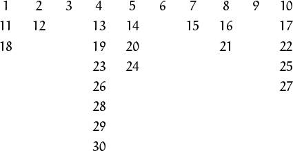
Suppose, for example, that we have n short lines of text that we’d like to arrange in m columns. For æsthetic reasons, we want the columns to be arranged in decreasing order of length (actually nonincreasing order); and the lengths should be approximately the same—no two columns should differ by more than one line’s worth of text. If 37 lines of text are being divided into five columns, we would therefore prefer the arrangement on the right:
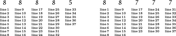
Furthermore we want to distribute the lines of text columnwise—first deciding how many lines go into the first column and then moving on to the second, the third, and so on—because that’s the way people read. Distributing row by row would give us the correct number of lines in each column, but the ordering would be wrong. (We would get something like the arrangement on the right, but column 1 would contain lines 1, 6, 11, . . . , 36, instead of lines 1, 2, 3, . . . , 8 as desired.)
A row-by-row distribution strategy can’t be used, but it does tell us how many lines to put in each column. If n is not a multiple of m, the rowby-row procedure makes it clear that the long columns should each contain ![]() n/m
n/m![]() lines, and the short columns should each contain
lines, and the short columns should each contain ![]() n/m
n/m![]() . There will be exactly n mod m long columns (and, as it turns out, there will be exactly n mumble m short ones).
. There will be exactly n mod m long columns (and, as it turns out, there will be exactly n mumble m short ones).
Let’s generalize the terminology and talk about ‘things’ and ‘groups’ instead of ‘lines’ and ‘columns’. We have just decided that the first group should contain ![]() n/m
n/m![]() things; therefore the following sequential distribution scheme ought to work: To distribute n things into m groups, when m > 0, put
things; therefore the following sequential distribution scheme ought to work: To distribute n things into m groups, when m > 0, put ![]() n/m
n/m![]() things into one group, then use the same procedure recursively to put the remaining n′ = n –
things into one group, then use the same procedure recursively to put the remaining n′ = n – ![]() n/m
n/m![]() things into m′ = m – 1 additional groups.
things into m′ = m – 1 additional groups.
For example, if n = 314 and m = 6, the distribution goes like this:
| remaining things | remaining groups | |
| 314 | 6 | 53 |
| 261 | 5 | 53 |
| 208 | 4 | 52 |
| 156 | 3 | 52 |
| 104 | 2 | 52 |
| 52 | 1 | 52 |
It works. We get groups of approximately the same size, even though the divisor keeps changing.
Why does it work? In general we can suppose that n = qm + r, where q = ![]() n/m
n/m![]() and r = n mod m. The process is simple if r = 0: We put
and r = n mod m. The process is simple if r = 0: We put ![]() n/m
n/m![]() = q things into the first group and replace n by n′ = n – q, leaving n′ = qm′ things to put into the remaining m′ = m – 1 groups. And if r > 0, we put
= q things into the first group and replace n by n′ = n – q, leaving n′ = qm′ things to put into the remaining m′ = m – 1 groups. And if r > 0, we put ![]() n/m
n/m![]() = q + 1 things into the first group and replace n by n′ = n – q – 1, leaving n′ = qm′ + r – 1 things for subsequent groups. The new remainder is r′ = r – 1, but q stays the same. It follows that there will be r groups with q + 1 things, followed by m – r groups with q things.
= q + 1 things into the first group and replace n by n′ = n – q – 1, leaving n′ = qm′ + r – 1 things for subsequent groups. The new remainder is r′ = r – 1, but q stays the same. It follows that there will be r groups with q + 1 things, followed by m – r groups with q things.
How many things are in the kth group? We’d like a formula that gives ![]() n/m
n/m![]() when k ≤ n mod m, and
when k ≤ n mod m, and ![]() n/m
n/m![]() otherwise. It’s not hard to verify that
otherwise. It’s not hard to verify that
has the desired properties, because this reduces to q + ![]() (r – k + 1)/m
(r – k + 1)/m![]() if we write n = qm + r as in the preceding paragraph; here q =
if we write n = qm + r as in the preceding paragraph; here q = ![]() n/m
n/m![]() . We have
. We have ![]() (r – k + 1)/m
(r – k + 1)/m![]() = [k ≤ r], if 1 ≤ k ≤ m and 0 ≤ r < m. Therefore we can write an identity that expresses the partition of n into m as-equal-as-possible parts in nonincreasing order:
= [k ≤ r], if 1 ≤ k ≤ m and 0 ≤ r < m. Therefore we can write an identity that expresses the partition of n into m as-equal-as-possible parts in nonincreasing order:
This identity is valid for all positive integers m, and for all integers n (whether positive, negative, or zero). We have already encountered the case m = 2 in (3.17), although we wrote it in a slightly different form, n = ![]() n/2
n/2![]() +
+ ![]() n/2
n/2![]() .
.
If we had wanted the parts to be in nondecreasing order, with the small groups coming before the larger ones, we could have proceeded in the same way but with ![]() n/m
n/m![]() things in the first group. Then we would have derived the corresponding identity
things in the first group. Then we would have derived the corresponding identity
It’s possible to convert between (3.25) and (3.24) by using either (3.4) or the identity of exercise 12.
Some claim that it’s too dangerous to replace anything by an mx.
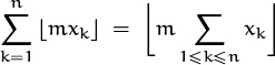
Now if we replace n in (3.25) by ![]() mx
mx![]() , and apply rule (3.11) to remove floors inside of floors, we get an identity that holds for all real x:
, and apply rule (3.11) to remove floors inside of floors, we get an identity that holds for all real x:
This is rather amazing, because the floor function is an integer approximation of a real value, but the single approximation on the left equals the sum of a bunch of them on the right. If we assume that ![]() x
x![]() is roughly
is roughly ![]() on the average, the left-hand side is roughly
on the average, the left-hand side is roughly ![]() , while the right-hand side comes to roughly
, while the right-hand side comes to roughly ![]() ; the sum of all these rough approximations turns out to be exact!
; the sum of all these rough approximations turns out to be exact!
3.5 Floor/Ceiling Sums
Equation (3.26) demonstrates that it’s possible to get a closed form for at least one kind of sum that involves ![]()
![]() . Are there others? Yes. The trick that usually works in such cases is to get rid of the floor or ceiling by introducing a new variable.
. Are there others? Yes. The trick that usually works in such cases is to get rid of the floor or ceiling by introducing a new variable.
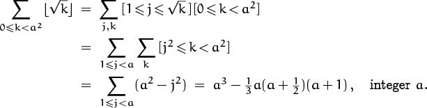
For example, let’s see if it’s possible to do the sum
in closed form. One idea is to introduce the variable ![]() ; we can do this “mechanically” by proceeding as we did in the roulette problem:
; we can do this “mechanically” by proceeding as we did in the roulette problem:
Once again the boundary conditions are a bit delicate. Let’s assume first that n = a2 is a perfect square. Then the second sum is zero, and the first can be evaluated by our usual routine:
Falling powers make the sum come tumbling down.
In the general case we can let ![]() ; then we merely need to add the terms for a2 ≤ k < n, which are all equal to a, so they sum to (n – a2)a. This gives the desired closed form,
; then we merely need to add the terms for a2 ≤ k < n, which are all equal to a, so they sum to (n – a2)a. This gives the desired closed form,
Another approach to such sums is to replace an expression of the form ![]() x
x![]() by ∑j[1 ≤ j ≤ x]; this is legal whenever x ≥ 0. Here’s how that method works in the sum of
by ∑j[1 ≤ j ≤ x]; this is legal whenever x ≥ 0. Here’s how that method works in the sum of ![]() square roots
square roots![]() , if we assume for convenience that n = a2:
, if we assume for convenience that n = a2:
Now here’s another example where a change of variable leads to a transformed sum. A remarkable theorem was discovered independently by three mathematicians—Bohl [34], Sierpiński [326], and Weyl [368]—at about the same time in 1909: If α is irrational then the fractional parts {nα} are very uniformly distributed between 0 and 1, as n → ∞. One way to state this is that

for all irrational α and all bounded functions f that are continuous almost everywhere. For example, the average value of {nα} can be found by setting f(x) = x; we get ![]() . (That’s exactly what we might expect; but it’s nice to know that it is really, provably true, no matter how irrational α is.)
. (That’s exactly what we might expect; but it’s nice to know that it is really, provably true, no matter how irrational α is.)
Warning: This stuff is fairly advanced. Better skim the next two pages on first reading; they aren’t crucial.
—Friendly TA
The theorem of Bohl, Sierpiński, and Weyl is proved by approximating f(x) above and below by “step functions,” which are linear combinations of the simple functions
fv(x) = [0 ≤ x < v]
when 0 ≤ v ≤ 1. Our purpose here is not to prove the theorem; that’s a job for calculus books. But let’s try to figure out the basic reason why it holds, by seeing how well it works in the special case f(x) = fv(x). In other words, let’s try to see how close the sum
gets to the “ideal” value nv, when n is large and α is irrational.
For this purpose we define the discrepancy D(α, n) to be the maximum absolute value, over all 0 ≤ v ≤ 1, of the sum
Our goal is to show that D(α, n) is “not too large” when compared with n, by showing that |s(α, n, v)| is always reasonably small when α is irrational. We can assume without loss of generality that 0 < α < 1.
First we can rewrite s(α, n, v) in simpler form, then introduce a new index variable j:

Right, name and conquer. The change of variable from k to j is the main point.
—Friendly TA
If we’re lucky, we can do the sum on k. But we ought to introduce some new variables, so that the formula won’t be such a mess. Let us write
| a = |
α–1 = | a + α′; |
| b = |
vα–1 = | b – v′ . |
Thus α′ = {α–1} is the fractional part of α–1, and v′ is the mumble-fractional part of vα–1.
Once again the boundary conditions are our only source of grief. For now, let’s forget the restriction ‘k < n’ and evaluate the sum on k without it:
OK, that’s pretty simple; we plug it in and plug away:
where S is a correction for the cases with k ≥ n that we have failed to exclude. The quantity jα′ will be an integer only when j = 0, since α (hence α′) is irrational; and jα′ – v′ will be an integer for at most one value of j. So we can change the ceiling terms to floors:
(The formula { 0 or 1} stands for something that’s either 0 or 1; we needn’t commit ourselves, because the details don’t really matter.)
Interesting. Instead of a closed form, we’re getting a sum that looks rather like s(α, n, v) but with different parameters: α′ instead of α, ![]() nα
nα![]() instead of n, and v′ instead of v. So we’ll have a recurrence for s(α, n, v), which (hopefully) will lead to a recurrence for the discrepancy D(α, n). This means we want to get
instead of n, and v′ instead of v. So we’ll have a recurrence for s(α, n, v), which (hopefully) will lead to a recurrence for the discrepancy D(α, n). This means we want to get
into the act:
s(α, n, v) = –nv + ![]() nα
nα![]() b –
b – ![]() nα
nα![]() v′ – s(α′,
v′ – s(α′, ![]() nα
nα![]() , v′) – S + {0 or 1} .
, v′) – S + {0 or 1} .
Recalling that b – v′ = vα–1, we see that everything will simplify beautifully if we replace ![]() nα
nα![]() (b – v′) by nα(b – v′) = nv:
(b – v′) by nα(b – v′) = nv:
s(α, n, v) = –s(α′, ![]() nα
nα![]() , v′) – S +
, v′) – S + ![]() + {0 or 1} .
+ {0 or 1} .
Here ![]() is a positive error less than vα–1. Exercise 18 proves that S is, similarly, between 0 and
is a positive error less than vα–1. Exercise 18 proves that S is, similarly, between 0 and ![]() vα–1
vα–1 ![]() . And we can remove the term for j =
. And we can remove the term for j = ![]() nα
nα![]() – 1 =
– 1 = ![]() nα
nα![]() from the sum, since it contributes either v′ or v′ – 1. Hence, if we take the maximum of absolute values over all v, we get
from the sum, since it contributes either v′ or v′ – 1. Hence, if we take the maximum of absolute values over all v, we get
The methods we’ll learn in succeeding chapters will allow us to conclude from this recurrence that D(α, n) is always much smaller than n, when n is sufficiently large. Hence theorem (3.28) is true; however, convergence to the limit is not always very fast. (See exercises 9.45 and 9.61.)

Whew; that was quite an exercise in manipulation of sums, floors, and ceilings. Readers who are not accustomed to “proving that errors are small” might find it hard to believe that anybody would have the courage to keep going, when faced with such weird-looking sums. But actually, a second look shows that there’s a simple motivating thread running through the whole calculation. The main idea is that a certain sum s(α, n, v) of n terms can be reduced to a similar sum of at most ![]() αn
αn![]() terms. Everything else cancels out except for a small residual left over from terms near the boundaries.
terms. Everything else cancels out except for a small residual left over from terms near the boundaries.
Let’s take a deep breath now and do one more sum, which is not trivial but has the great advantage (compared with what we’ve just been doing) that it comes out in closed form so that we can easily check the answer. Our goal now will be to generalize the sum in (3.26) by finding an expression for
Is this a harder sum of floors, or a sum of harder floors?
Finding a closed form for this sum is tougher than what we’ve done so far (except perhaps for the discrepancy problem we just looked at). But it’s instructive, so we’ll hack away at it for the rest of this chapter.
As usual, especially with tough problems, we start by looking at small cases. The special case n = 1 is (3.26), with x replaced by x/m:
Be forewarned: This is the beginning of a pattern, in that the last part of the chapter consists of the solution of some long, difficult problem, with little more motivation than curiosity.
—Students
And as in Chapter 1, we find it useful to get more data by generalizing downwards to the case n = 0:
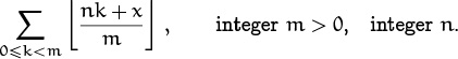
Touché. But c’mon, gang, do you always need to be told about applications before you can get interested in something? This sum arises, for example, in the study of random number generation and testing. But mathematicians looked at it long before computers came along, because they found it natural to ask if there’s a way to sum arithmetic progressions that have been “floored.”
—Your instructor
Our problem has two parameters, m and n; let’s look at some small cases for m. When m = 1 there’s just a single term in the sum and its value is ![]() x
x![]() . When m = 2 the sum is
. When m = 2 the sum is ![]() x/2
x/2![]() +
+ ![]() (x + n)/2
(x + n)/2![]() . We can remove the interaction between x and n by removing n from inside the floor function, but to do that we must consider even and odd n separately. If n is even, n/2 is an integer, so we can remove it from the floor:
. We can remove the interaction between x and n by removing n from inside the floor function, but to do that we must consider even and odd n separately. If n is even, n/2 is an integer, so we can remove it from the floor:
If n is odd, (n – 1)/2 is an integer so we get
The last step follows from (3.26) with m = 2.
These formulas for even and odd n slightly resemble those for n = 0 and 1, but no clear pattern has emerged yet; so we had better continue exploring some more small cases. For m = 3 the sum is
and we consider three cases for n: Either it’s a multiple of 3, or it’s 1 more than a multiple, or it’s 2 more. That is, n mod 3 = 0, 1, or 2. If n mod 3 = 0 then n/3 and 2n/3 are integers, so the sum is
If n mod 3 = 1 then (n – 1)/3 and (2n – 2)/3 are integers, so we have
Again this last step follows from (3.26), this time with m = 3. And finally, if n mod 3 = 2 then
The left hemispheres of our brains have finished the case m = 3, but the right hemispheres still can’t recognize the pattern, so we proceed to m = 4:
“Inventive genius requires pleasurable mental activity as a condition for its vigorous exercise. ‘Necessity is the mother of invention’ is a silly proverb. ‘Necessity is the mother of futile dodges’ is much nearer to the truth. The basis of the growth of modern invention is science, and science is almost wholly the outgrowth of pleasurable intellectual curiosity.”
—A. N. White-head [371]
At least we know enough by now to consider cases based on n mod m. If n mod 4 = 0 then
And if n mod 4 = 1,
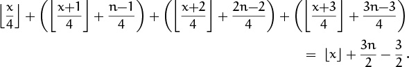
The case n mod 4 = 3 turns out to give the same answer. Finally, in the case n mod 4 = 2 we get something a bit different, and this turns out to be an important clue to the behavior in general:
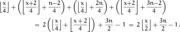
This last step simplifies something of the form ![]() y/2
y/2![]() +
+ ![]() (y + 1)/2
(y + 1)/2![]() , which again is a special case of (3.26).
, which again is a special case of (3.26).
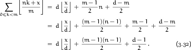
To summarize, here’s the value of our sum for small m:
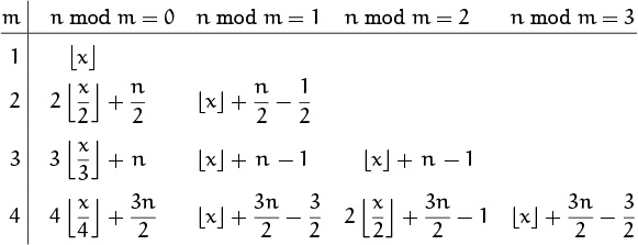
It looks as if we’re getting something of the form
where a, b, and c somehow depend on m and n. Even the myopic among us can see that b is probably (m – 1)/2. It’s harder to discern an expression for a; but the case n mod 4 = 2 gives us a hint that a is probably gcd(m, n), the greatest common divisor of m and n. This makes sense because gcd(m, n) is the factor we remove from m and n when reducing the fraction n/m to lowest terms, and our sum involves the fraction n/m. (We’ll look carefully at gcd operations in Chapter 4.) The value of c seems more mysterious, but perhaps it will drop out of our proofs for a and b.
In computing the sum for small m, we’ve effectively rewritten each term of the sum as
because (kn – kn mod m)/m is an integer that can be removed from inside the floor brackets. Thus the original sum can be expanded into the following tableau:
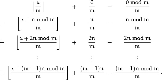
When we experimented with small values of m, these three columns led respectively to a![]() x/a
x/a![]() , bn, and c.
, bn, and c.
In particular, we can see how b arises. The second column is an arithmetic progression, whose sum we know—it’s the average of the first and last terms, times the number of terms:
So our guess that b = (m – 1)/2 has been verified.
The first and third columns seem tougher; to determine a and c we must take a closer look at the sequence of numbers
0 mod m, n mod m, 2n mod m, . . . , (m – 1)n mod m.
Suppose, for example, that m = 12 and n = 5. If we think of the sequence as times on a clock, the numbers are 0 o’clock (we take 12 o’clock to be 0 o’clock), then 5 o’clock, 10 o’clock, 3 o’clock (= 15 o’clock), 8 o’clock, and so on. It turns out that we hit every hour exactly once.
Now suppose m = 12 and n = 8. The numbers are 0 o’clock, 8 o’clock, 4 o’clock (= 16 o’clock), but then 0, 8, and 4 repeat. Since both 8 and 12 are multiples of 4, and since the numbers start at 0 (also a multiple of 4), there’s no way to break out of this pattern—they must all be multiples of 4.
In these two cases we have gcd(12, 5) = 1 and gcd(12, 8) = 4. The general rule, which we will prove next chapter, states that if d = gcd(m, n) then we get the numbers 0, d, 2d, . . . , m – d in some order, followed by d – 1 more copies of the same sequence. For example, with m = 12 and n = 8 the pattern 0, 8, 4 occurs four times.
Lemma now, dilemma later.
The first column of our sum now makes complete sense. It contains d copies of the terms ![]() x/m
x/m![]() ,
, ![]() (x + d)/m
(x + d)/m![]() , . . . ,
, . . . , ![]() (x + m – d)/m
(x + m – d)/m![]() , in some order, so its sum is
, in some order, so its sum is
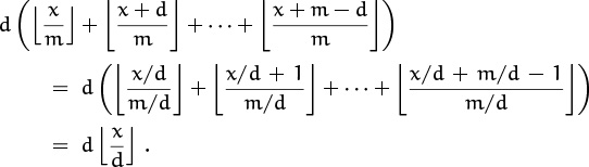
This last step is yet another application of (3.26). Our guess for a has been verified:
a = d = gcd(m, n) .
Also, as we guessed, we can now compute c, because the third column has become easy to fathom. It contains d copies of the arithmetic progression 0/m, d/m, 2d/m, . . . , (m – d)/m, so its sum is
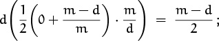
the third column is actually subtracted, not added, so we have
End of mystery, end of quest. The desired closed form is
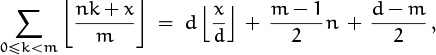
where d = gcd(m, n). As a check, we can make sure this works in the special cases n = 0 and n = 1 that we knew before: When n = 0 we get d = gcd(m, 0) = m; the last two terms of the formula are zero so the formula properly gives m![]() x/m
x/m![]() . And for n = 1 we get d = gcd(m, 1) = 1; the last two terms cancel nicely, and the sum is just
. And for n = 1 we get d = gcd(m, 1) = 1; the last two terms cancel nicely, and the sum is just ![]() x
x![]() .
.
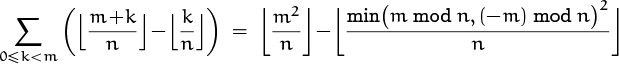
By manipulating the closed form a bit, we can actually make it symmetric in m and n:
This is astonishing, because there’s no algebraic reason to suspect that such a sum should be symmetrical. We have proved a “reciprocity law,”
Yup, I’m floored.
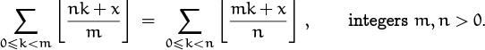
For example, if m = 41 and n = 127, the left sum has 41 terms and the right has 127; but they still come out equal, for all real x.
Exercises
Warmups
1. When we analyzed the Josephus problem in Chapter 1, we represented an arbitrary positive integer n in the form n = 2m +l, where 0 ≤ l < 2m. Give explicit formulas for l and m as functions of n, using floor and/or ceiling brackets.
2. What is a formula for the nearest integer to a given real number x? In case of ties, when x is exactly halfway between two integers, give an expression that rounds (a) up—that is, to ![]() x
x![]() ; (b) down—that is, to
; (b) down—that is, to ![]() x
x![]() .
.
3. Evaluate ![]()
![]() mα
mα![]() n/α
n/α![]() , when m and n are positive integers and α is an irrational number greater than n.
, when m and n are positive integers and α is an irrational number greater than n.
4. The text describes problems at levels 1 through 5. What is a level 0 problem? (This, by the way, is not a level 0 problem.)
5. Find a necessary and sufficient condition that ![]() nx
nx![]() = n
= n![]() x
x![]() , when n is a positive integer. (Your condition should involve {x}.)
, when n is a positive integer. (Your condition should involve {x}.)
6. Can something interesting be said about ![]() f(x)
f(x)![]() when f(x) is a continuous, monotonically decreasing function that takes integer values only when x is an integer?
when f(x) is a continuous, monotonically decreasing function that takes integer values only when x is an integer?
7. Solve the recurrence
Xn = n, for 0 ≤ n < m;
Xn = Xn–m + 1, for n ≥ m.
8. Prove the Dirichlet box principle: If n objects are put into m boxes, some box must contain ≥ ![]() n/m
n/m![]() objects, and some box must contain ≤
objects, and some box must contain ≤ ![]() n/m
n/m![]() .
.
You know you’re in college when the book doesn’t tell you how to pronounce ‘Dirichlet’.
9. Egyptian mathematicians in 1800 B.C. represented rational numbers between 0 and 1 as sums of unit fractions 1/x1 + · · · + 1/xk, where the x’s were distinct positive integers. For example, they wrote ![]() instead of
instead of ![]() . Prove that it is always possible to do this in a systematic way: If 0 < m/n < 1, then
. Prove that it is always possible to do this in a systematic way: If 0 < m/n < 1, then
(This is Fibonacci’s algorithm, due to Leonardo Fibonacci, A.D. 1202.)
Basics
10. Show that the expression
is always either ![]() x
x![]() or
or ![]() x
x![]() . In what circumstances does each case arise?
. In what circumstances does each case arise?
11. Give details of the proof alluded to in the text, that the open interval (α . . β) contains exactly ![]() β
β![]() –
– ![]() α
α![]() – 1 integers when α < β. Why does the case α = β have to be excluded in order to make the proof correct?
– 1 integers when α < β. Why does the case α = β have to be excluded in order to make the proof correct?
12. Prove that
for all integers n and all positive integers m. [This identity gives us another way to convert ceilings to floors and vice versa, instead of using the reflective law (3.4).]
13. Let α and β be positive real numbers. Prove that Spec(α) and Spec(β) partition the positive integers if and only if α and β are irrational and 1/α + 1/β = 1.
14. Prove or disprove:
(x mod ny) mod y = x mod y, integer n.
15. Is there an identity analogous to (3.26) that uses ceilings instead of floors?
16. Prove that n mod 2 = (1–(–1)n)/2. Find and prove a similar expression for n mod 3 in the form a+bωn +cω2n, where ω is the complex number ![]() . Hint: ω3 = 1 and 1 + ω + ω2 = 0.
. Hint: ω3 = 1 and 1 + ω + ω2 = 0.
17. Evaluate the sum ∑0≤k<m![]() x + k/m
x + k/m![]() in the case x ≥ 0 by substituting ∑j[1 ≤ j ≤ x + k/m] for
in the case x ≥ 0 by substituting ∑j[1 ≤ j ≤ x + k/m] for ![]() x + k/m
x + k/m![]() and summing first on k. Does your answer agree with (3.26)?
and summing first on k. Does your answer agree with (3.26)?
18. Prove that the boundary-value error term S in (3.30) is at most ![]() α–1v
α–1v![]() . Hint: Show that small values of j are not involved.
. Hint: Show that small values of j are not involved.
Homework exercises
19. Find a necessary and sufficient condition on the real number b > 1 such that
![]() logb x
logb x![]() =
= ![]() logb
logb![]() x
x![]()
![]()
for all real x ≥ 1.
20. Find the sum of all multiples of x in the closed interval [α . . β], when x > 0.
21. How many of the numbers 2m, for 0 ≤ m ≤ M, have leading digit 1 in decimal notation?
22. Evaluate the sums ![]() and
and ![]() .
.
23. Show that the nth element of the sequence
1, 2, 2, 3, 3, 3, 4, 4, 4, 4, 5, 5, 5, 5, 5, . . .
is ![]() . (The sequence contains exactly m occurrences of m.)
. (The sequence contains exactly m occurrences of m.)
24. Exercise 13 establishes an interesting relation between the two multisets Spec(α) and Spec (α/(α – 1)), when α is any irrational number > 1, because 1/α + (α – 1)/α = 1. Find (and prove) an interesting relation between the two multisets Spec(α) and Spec (α/(α + 1)), when α is any positive real number.
25. Prove or disprove that the Knuth numbers, defined by (3.16), satisfy Kn ≥ n for all nonnegative n.
26. Show that the auxiliary Josephus numbers (3.20) satisfy
27. Prove that infinitely many of the numbers ![]() defined by (3.20) are even, and that infinitely many are odd.
defined by (3.20) are even, and that infinitely many are odd.
28. Solve the recurrence
a0 = 1;
an = an–1 + ![]()
![]()
![]() , for n > 0.
, for n > 0.
29. Show that, in addition to (3.31), we have
D(α, n) ≥ D(α′, ![]() αn
αn![]() ) – α–1 – 2.
) – α–1 – 2.
There’s a discrepancy between this formula and (3.31).
30. Show that the recurrence
X0 = m,
Xn = ![]() – 2, for n > 0,
– 2, for n > 0,
has the solution Xn = ![]() α2n
α2n![]() , if m is an integer greater than 2, where α + α–1 = m and α > 1. For example, if m = 3 the solution is
, if m is an integer greater than 2, where α + α–1 = m and α > 1. For example, if m = 3 the solution is
31. Prove or disprove: ![]() x
x![]() +
+ ![]() y
y![]() +
+ ![]() x + y
x + y![]() ≤
≤ ![]() 2x
2x![]() +
+ ![]() 2y
2y![]() .
.
32. Let ∥x∥ = min (x – ![]() x
x![]() ,
, ![]() x
x![]() – x) denote the distance from x to the nearest integer. What is the value of
– x) denote the distance from x to the nearest integer. What is the value of
(Note that this sum can be doubly infinite. For example, when x = 1/3 the terms are nonzero as k → –∞ and also as k → +∞ .)
Exam problems
33. A circle, 2n – 1 units in diameter, has been drawn symmetrically on a 2n × 2n chessboard, illustrated here for n = 3:
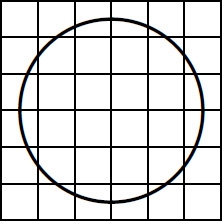
a. How many cells of the board contain a segment of the circle?
b. Find a function f(n, k) such that exactly ![]() cells of the board lie entirely within the circle.
cells of the board lie entirely within the circle.
34. Let ![]() .
.
a. Find a closed form for f(n), when n ≥ 1.
b. Prove that f(n) = n – 1 + f(![]() n/2
n/2![]() ) + f (
) + f (![]() n/2
n/2![]() ) for all n ≥ 1.
) for all n ≥ 1.
35. Simplify the formula ![]() (n + 1)2n!e
(n + 1)2n!e![]() mod n.
mod n.
Simplify it, but don’t change the value.
36. Assuming that n is a nonnegative integer, find a closed form for the sum

37. Prove the identity
for all positive integers m and n.
38. Let x1, . . . , xn be real numbers such that the identity
holds for all positive integers m. Prove something interesting about x1, . . . , xn.
39. Prove that the double sum ∑0≤k≤logbx ∑0<j<b![]() (x + jbk)/bk+1
(x + jbk)/bk+1![]() equals (b – 1) (
equals (b – 1) (![]() logb x
logb x![]() + 1) +
+ 1) + ![]() x
x![]() – 1, for every real number x ≥ 1 and every integer b > 1.
– 1, for every real number x ≥ 1 and every integer b > 1.
40. The spiral function σ(n), indicated in the diagram below, maps a nonnegative integer n onto an ordered pair of integers (x(n), y(n)). For example, it maps n = 9 onto the ordered pair (1, 2).
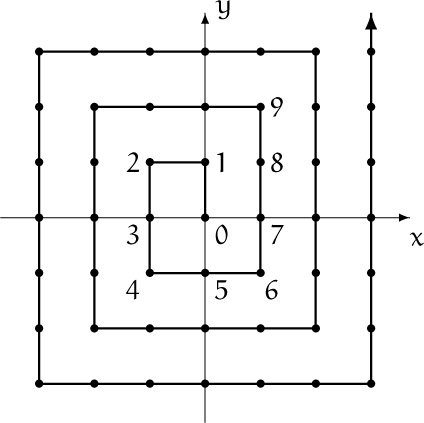
People in the southern hemisphere use a different spiral.
a. Prove that if ![]() ,
,
and find a similar formula for y(n). Hint: Classify the spiral into segments Wk, Sk, Ek, Nk according as ![]() , 4k – 1, 4k, 4k + 1.
, 4k – 1, 4k, 4k + 1.
b. Prove that, conversely, we can determine n from σ(n) by a formula of the form
n = (2k)2 ± (2k + x(n) + y(n)) , k = max (|x(n)|, |y(n)|) .
Give a rule for when the sign is + and when the sign is –.
Bonus problems
41. Let f and g be increasing functions such that the sets {f(1), f(2), . . . } and {g(1), g(2), . . . } partition the positive integers. Suppose that f and g are related by the condition g(n) = f(f(n)) + 1 for all n > 0. Prove that f(n) = ![]() nϕ
nϕ![]() and g(n) =
and g(n) = ![]() nϕ2
nϕ2![]() , where
, where ![]() .
.
42. Do there exist real numbers α, β, and γ such that Spec(α), Spec(β), and Spec(γ) together partition the set of positive integers?
43. Find an interesting interpretation of the Knuth numbers, by unfolding the recurrence (3.16).
44. Show that there are integers ![]() and
and ![]() such that
such that

when ![]() is the solution to (3.20). Use this fact to obtain another form of the solution to the generalized Josephus problem:
is the solution to (3.20). Use this fact to obtain another form of the solution to the generalized Josephus problem:
45. Extend the trick of exercise 30 to find a closed-form solution to
Y0 = m,
Yn = ![]() – 1, for n > 0,
– 1, for n > 0,
if m is a positive integer.
46. Prove that if ![]() , where m and l are nonnegative integers, then
, where m and l are nonnegative integers, then ![]() . Use this remarkable property to find a closed form solution to the recurrence
. Use this remarkable property to find a closed form solution to the recurrence
Hint: ![]() .
.
47. The function f(x) is said to be replicative if it satisfies
for every positive integer m. Find necessary and sufficient conditions on the real number c for the following functions to be replicative:
a. f(x) = x + c.
b. f(x) = [x + c is an integer].
c. f(x) = max(![]() x
x![]() , c).
, c).
d. f(x) = x + c![]() x
x![]() –
– ![]() [x is not an integer].
[x is not an integer].
48. Prove the identity
x3 = 3x ![]() x
x![]() x
x![]()
![]() + 3{x} {x
+ 3{x} {x![]() x
x![]() } + {x}3 – 3
} + {x}3 – 3![]() x
x![]()
![]() x
x![]() x
x![]()
![]() +
+ ![]() x
x![]() 3 ,
3 ,
and show how to obtain similar formulas for xn when n > 3.
49. Find a necessary and sufficient condition on the real numbers 0 ≤ α < 1 and β ≥ 0 such that we can determine α and β from the infinite multiset of values
{![]() nα
nα![]() +
+ ![]() nβ
nβ![]() | n > 0}.
| n > 0}.
Research problems
50. Find a necessary and sufficient condition on the nonnegative real numbers α and β such that we can determine α and β from the infinite multiset of values
{![]()
![]() nα
nα![]() β
β![]() | n > 0}.
| n > 0}.
51. Let x be a real number ≥ ![]() . The solution to the recurrence
. The solution to the recurrence
Z0(x) = x,
Zn(x) = Zn–1(x)2 – 1, for n > 0,
can be written Zn(x) = ![]() f(x)2n
f(x)2n![]() , if x is an integer, where
, if x is an integer, where
because Zn(x) – 1 < f(x)2n < Zn(x) in that case. What other interesting properties does this function f(x) have?
52. Given nonnegative real numbers α and β, let
Spec(α; β) = {![]() α + β
α + β![]() ,
, ![]() 2α + β
2α + β![]() ,
, ![]() 3α + β
3α + β![]() , . . . }
, . . . }
be a multiset that generalizes Spec(α) = Spec(α; 0). Prove or disprove: If the m ≥ 3 multisets Spec(α1; β1), Spec(α2; β2), . . . , Spec(αm; βm) partition the positive integers, and if the parameters α1 < α2 < · · · < αm are rational, then
Spec this be hard.
53. Fibonacci’s algorithm (exercise 9) is “greedy” in the sense that it chooses the least conceivable q at every step. A more complicated algorithm is known by which every fraction m/n with n odd can be represented as a sum of distinct unit fractions 1/q1 + · · · + 1/qk with odd denominators. Does the greedy algorithm for such a representation always terminate?