5. Binomial Coefficients

Let’s take a breather. The previous chapters have seen some heavy going, with sums involving floor, ceiling, mod, phi, and mu functions. Now we’re going to study binomial coefficients, which turn out to be (a) more important in applications, and (b) easier to manipulate, than all those other quantities.

Lucky us!

5.1 Basic Identities

The symbol is a binomial coefficient, so called because of an important property we look at later this section, the binomial theorem. But we read the symbol “n choose k.” This incantation arises from its combinatorial interpretation—it is the number of ways to choose a k-element subset from an n-element set. For example, from the set {1, 2, 3, 4} we can choose two elements in six ways,

{1, 2} , {1, 3} , {1, 4} , {2, 3} , {2, 4} , {3, 4};

Otherwise known as combinations of n things, k at a time.

so .

To express the number in more familiar terms it’s easiest to first determine the number of k-element sequences, rather than subsets, chosen from an n-element set; for sequences, the order of the elements counts. We use the same argument we used in Chapter 4 to show that n! is the number of permutations of n objects. There are n choices for the first element of the sequence; for each, there are n–1 choices for the second; and so on, until there are n–k+1 choices for the kth. This gives n(n–1) . . . (n–k+1) = n^k choices in all. And since each k-element subset has exactly k! different orderings, this number of sequences counts each subset exactly k! times. To get our answer, we simply divide by k!:

For example,

this agrees with our previous enumeration.

We call n the upper index and k the lower index. The indices are restricted to be nonnegative integers by the combinatorial interpretation, because sets don’t have negative or fractional numbers of elements. But the binomial coefficient has many uses besides its combinatorial interpretation, so we will remove some of the restrictions. It’s most useful, it turns out, to allow an arbitrary real (or even complex) number to appear in the upper index, and to allow an arbitrary integer in the lower. Our formal definition therefore takes the following form:

This definition has several noteworthy features. First, the upper index is called r, not n; the letter r emphasizes the fact that binomial coefficients make sense when any real number appears in this position. For instance, we have . There’s no combinatorial interpretation here, but r = –1 turns out to be an important special case. A noninteger index like r = –1/2 also turns out to be useful.

Second, we can view as a kth-degree polynomial in r. We’ll see that this viewpoint is often helpful.

Third, we haven’t defined binomial coefficients for noninteger lower indices. A reasonable definition can be given, but actual applications are rare, so we will defer this generalization to later in the chapter.

Final note: We’ve listed the restrictions ‘integer k ≥ 0’ and ‘integer k < 0’ at the right of the definition. Such restrictions will be listed in all the identities we will study, so that the range of applicability will be clear. In general the fewer restrictions the better, because an unrestricted identity is most useful; still, any restrictions that apply are an important part of the identity. When we manipulate binomial coefficients, it’s easier to ignore difficult-to-remember restrictions temporarily and to check later that nothing has been violated. But the check needs to be made.

For example, almost every time we encounter it equals 1, so we can get lulled into thinking that it’s always 1. But a careful look at definition (5.1) tells us that is 1 only when n ≥ 0 (assuming that n is an integer); when n < 0 we have . Traps like this can (and will) make life adventuresome.

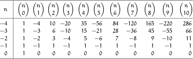
Before getting to the identities that we will use to tame binomial coefficients, let’s take a peek at some small values. The numbers in Table 155 form the beginning of Pascal’s triangle, named after Blaise Pascal (1623–1662)

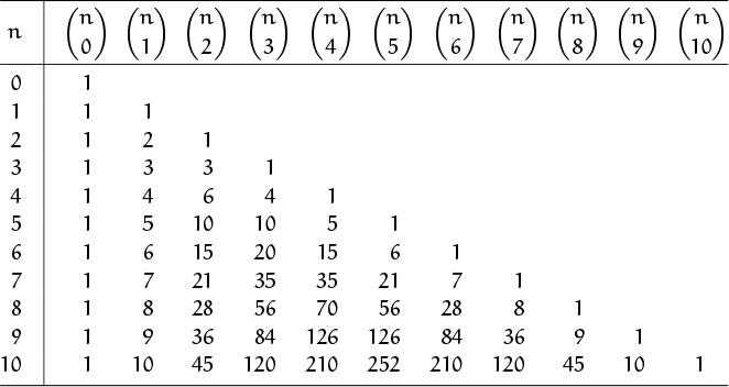
because he wrote an influential treatise about them [285]. The empty entries in this table are actually 0’s, because of a zero in the numerator of (5.1); for example, . These entries have been left blank simply to help emphasize the rest of the table.

Binomial coefficients were well known in Asia, many centuries before Pascal was born [90], but he had no way to know that.

It’s worthwhile to memorize formulas for the first three columns,

these hold for arbitrary reals. (Recall that is the formula we derived for triangular numbers in Chapter 1; triangular numbers are conspicuously present in the column of Table 155.) It’s also a good idea to memorize the first five rows or so of Pascal’s triangle, so that when the pattern 1, 4, 6, 4, 1 appears in some problem we will have a clue that binomial coefficients probably lurk nearby.

The numbers in Pascal’s triangle satisfy, practically speaking, infinitely many identities, so it’s not too surprising that we can find some surprising relationships by looking closely. For example, there’s a curious “hexagon property,” illustrated by the six numbers 56, 28, 36, 120, 210, 126 that surround 84 in the lower right portion of Table 155. Both ways of multiplying alternate numbers from this hexagon give the same product: 56·36·210 = 28·120·126 = 423360. The same thing holds if we extract such a hexagon from any other part of Pascal’s triangle.

In Italy it’s called Tartaglia’s triangle.

And now the identities. Our goal in this section will be to learn a few simple rules by which we can solve the vast majority of practical problems involving binomial coefficients.

“C’est une chose estrange combien il est fertile en proprietez.”

—B. Pascal [285]

Definition (5.1) can be recast in terms of factorials in the common case that the upper index r is an integer, n, that’s greater than or equal to the lower index k:

To get this formula, we just multiply the numerator and denominator of (5.1) by (n – k)!. It’s occasionally useful to expand a binomial coefficient into this factorial form (for example, when proving the hexagon property). And we often want to go the other way, changing factorials into binomials.

The factorial representation hints at a symmetry in Pascal’s triangle: Each row reads the same left-to-right as right-to-left. The identity reflecting this—called the symmetry identity—is obtained by changing k to n – k:

This formula makes combinatorial sense, because by specifying the k chosen things out of n we’re in effect specifying the n – k unchosen things.

The restriction that n and k be integers in identity (5.4) is obvious, since each lower index must be an integer. But why can’t n be negative? Suppose, for example, that n = –1. Is

a valid equation? No. For instance, when k = 0 we get 1 on the left and 0 on the right. In fact, for any integer k ≥ 0 the left side is

which is either 1 or –1; but the right side is 0, because the lower index is negative. And for negative k the left side is 0 but the right side is

which is either 1 or –1. So the equation is always false!

The symmetry identity fails for all other negative integers n, too. But unfortunately it’s all too easy to forget this restriction, since the expression in the upper index is sometimes negative only for obscure (but legal) values of its variables. Everyone who’s manipulated binomial coefficients much has fallen into this trap at least three times.

I just hope I don’t fall into this trap during the midterm.

But the symmetry identity does have a big redeeming feature: It works for all values of k, even when k < 0 or k > n. (Because both sides are zero in such cases.) Otherwise 0 ≤ k ≤ n, and symmetry follows immediately from (5.3):

Our next important identity lets us move things in and out of binomial coefficients:

The restriction on k prevents us from dividing by 0 here. We call (5.5) an absorption identity, because we often use it to absorb a variable into a binomial coefficient when that variable is a nuisance outside. The equation follows from definition (5.1), because r^k = r(r – 1)^k–1 and k! = k(k – 1)! when k > 0; both sides are zero when k < 0.

If we multiply both sides of (5.5) by k, we get an absorption identity that works even when k = 0:

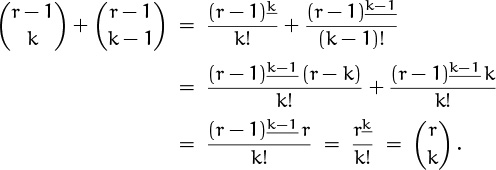
This one also has a companion that keeps the lower index intact:

We can derive (5.7) by sandwiching an application of (5.6) between two applications of symmetry:

But wait a minute. We’ve claimed that the identity holds for all real r, yet the derivation we just gave holds only when r is a positive integer. (The upper index r – 1 must be a nonnegative integer if we’re to use the symmetry property (5.4) with impunity.) Have we been cheating? No. It’s true that the derivation is valid only for positive integers r; but we can claim that the identity holds for all values of r, because both sides of (5.7) are polynomials in r of degree k + 1. A nonzero polynomial of degree d or less can have at most d distinct zeros; therefore the difference of two such polynomials, which also has degree d or less, cannot be zero at more than d points unless it is identically zero. In other words, if two polynomials of degree d or less agree at more than d points, they must agree everywhere. We have shown that whenever r is a positive integer; so these two polynomials agree at infinitely many points, and they must be identically equal.

(Well, not here anyway.)

The proof technique in the previous paragraph, which we will call the polynomial argument, is useful for extending many identities from integers to reals; we’ll see it again and again. Some equations, like the symmetry identity (5.4), are not identities between polynomials, so we can’t always use this method. But many identities do have the necessary form.

For example, here’s another polynomial identity, perhaps the most important binomial identity of all, known as the addition formula:

When r is a positive integer, the addition formula tells us that every number in Pascal’s triangle is the sum of two numbers in the previous row, one directly above it and the other just to the left. And the formula applies also when r is negative, real, or complex; the only restriction is that k be an integer, so that the binomial coefficients are defined.

One way to prove the addition formula is to assume that r is a positive integer and to use the combinatorial interpretation. Recall that is the number of possible k-element subsets chosen from an r-element set. If we have a set of r eggs that includes exactly one bad egg, there are ways to select k of the eggs. Exactly of these selections involve nothing but good eggs; and of them contain the bad egg, because such selections have k – 1 of the r – 1 good eggs. Adding these two numbers together gives (5.8). This derivation assumes that r is a positive integer, and that k ≥ 0. But both sides of the identity are zero when k < 0, and the polynomial argument establishes (5.8) in all remaining cases.

We can also derive (5.8) by adding together the two absorption identities (5.7) and (5.6):

the left side is , and we can divide through by r. This derivation is valid for everything but r = 0, and it’s easy to check that remaining case.

Those of us who tend not to discover such slick proofs, or who are otherwise into tedium, might prefer to derive (5.8) by a straightforward manipulation of the definition. If k > 0,

Again, the cases for k ≤ 0 are easy to handle.

We’ve just seen three rather different proofs of the addition formula. This is not surprising; binomial coefficients have many useful properties, several of which are bound to lead to proofs of an identity at hand.

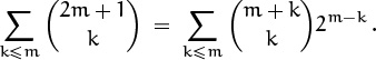
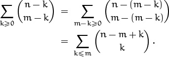
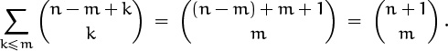
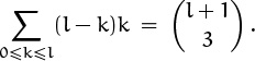
The addition formula is essentially a recurrence for the numbers of Pascal’s triangle, so we’ll see that it is especially useful for proving other identities by induction. We can also get a new identity immediately by unfolding the recurrence. For example,

Since , that term disappears and we can stop. This method yields the general formula

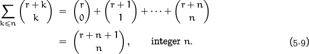
Notice that we don’t need the lower limit k ≥ 0 on the index of summation, because the terms with k < 0 are zero.

This formula expresses one binomial coefficient as the sum of others whose upper and lower indices stay the same distance apart. We found it by repeatedly expanding the binomial coefficient with the smallest lower index: first , then , then , then . What happens if we unfold the other way, repeatedly expanding the one with largest lower index? We get

Now is zero (so are and , but these make the identity nicer), and we can spot the general pattern:

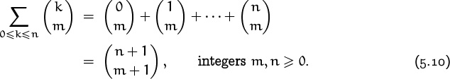
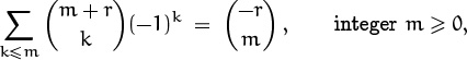
This identity, which we call summation on the upper index, expresses a binomial coefficient as the sum of others whose lower indices are constant. In this case the sum needs the lower limit k ≥ 0, because the terms with k < 0 aren’t zero. Also, m and n can’t in general be negative.

Identity (5.10) has an interesting combinatorial interpretation. If we want to choose m + 1 tickets from a set of n + 1 tickets numbered 0 through n, there are ways to do this when the largest ticket selected is number k.

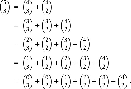
We can prove both (5.9) and (5.10) by induction using the addition formula, but we can also prove them from each other. For example, let’s prove (5.9) from (5.10); our proof will illustrate some common binomial coefficient manipulations. Our general plan will be to massage the left side of (5.9) so that it looks like the left side of (5.10); then we’ll invoke that identity, replacing the sum by a single binomial coefficient; finally we’ll transform that coefficient into the right side of (5.9).

We can assume for convenience that r and n are nonnegative integers; the general case of (5.9) follows from this special case, by the polynomial argument. Let’s write m instead of r, so that this variable looks more like a nonnegative integer. The plan can now be carried out systematically as follows:

Let’s look at this derivation blow by blow. The key step is in the second line, where we apply the symmetry law (5.4) to replace by . We’re allowed to do this only when m + k ≥ 0, so our first step restricts the range of k by discarding the terms with k < –m. (This is legal because those terms are zero.) Now we’re almost ready to apply (5.10); the third line sets this up, replacing k by k – m and tidying up the range of summation. This step, like the first, merely plays around with ∑-notation. Now k appears by itself in the upper index and the limits of summation are in the proper form, so the fourth line applies (5.10). One more use of symmetry finishes the job.

Certain sums that we did in Chapters 1 and 2 were actually special cases of (5.10), or disguised versions of this identity. For example, the case m = 1 gives the sum of the nonnegative integers up through n:

And the general case is equivalent to Chapter 2’s rule

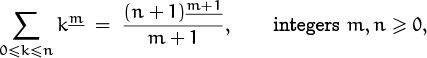
if we divide both sides of this formula by m!. In fact, the addition formula (5.8) tells us that

if we replace r and k respectively by x + 1 and m. Hence the methods of Chapter 2 give us the handy indefinite summation formula

Binomial coefficients get their name from the binomial theorem, which deals with powers of the binomial expression x + y. Let’s look at the smallest cases of this theorem:

“At the age of twenty-one he [Moriarty] wrote a treatise upon the Binomial Theorem, which has had a European vogue. On the strength of it, he won the Mathematical Chair at one of our smaller Universities.”

—S. Holmes [84]

(x + y)⁰ = 1x⁰y⁰

(x + y)¹ = 1x¹y⁰ + 1x⁰y¹

(x + y)² = 1x²y⁰ + 2x¹y¹ + 1x⁰y²

(x + y)³ = 1x³y⁰ + 3x²y¹ + 3x¹y² + 1x⁰y³

(x + y)⁴ = 1x⁴y⁰ + 4x³y¹ + 6x²y² + 4x¹y³ + 1x⁰y⁴ .

It’s not hard to see why these coefficients are the same as the numbers in Pascal’s triangle: When we expand the product

every term is itself the product of n factors, each either an x or y. The number of such terms with k factors of x and n – k factors of y is the coefficient of x^ky^n–k after we combine like terms. And this is exactly the number of ways to choose k of the n binomials from which an x will be contributed; that is, it’s .

Some textbooks leave the quantity 0⁰ undefined, because the functions x⁰ and 0^x have different limiting values when x decreases to 0. But this is a mistake. We must define

x⁰ = 1,      for all x,

if the binomial theorem is to be valid when x = 0, y = 0, and/or x = –y. The theorem is too important to be arbitrarily restricted! By contrast, the function 0^x is quite unimportant. (See [220] for further discussion.)

But what exactly is the binomial theorem? In its full glory it is the following identity:

The sum is over all integers k; but it is really a finite sum when r is a nonnegative integer, because all terms are zero except those with 0 ≤ k ≤ r. On the other hand, the theorem is also valid when r is negative, or even when r is an arbitrary real or complex number. In such cases the sum really is infinite, unless r is a nonnegative integer, and we must have |x/y| < 1 to guarantee the sum’s absolute convergence.

Two special cases of the binomial theorem are worth special attention, even though they are extremely simple. If x = y = 1 and r = n is nonnegative, we get

This equation tells us that row n of Pascal’s triangle sums to 2ⁿ. And when x is –1 instead of +1, we get

For example, 1 – 4 + 6 – 4 + 1 = 0; the elements of row n sum to zero if we give them alternating signs, except in the top row (when n = 0 and 0⁰ = 1).

When r is not a nonnegative integer, we most often use the binomial theorem in the special case y = 1. Let’s state this special case explicitly, writing z instead of x to emphasize the fact that an arbitrary complex number can be involved here:

The general formula in (5.12) follows from this one if we set z = x/y and multiply both sides by y^r.

We have proved the binomial theorem only when r is a nonnegative integer, by using a combinatorial interpretation. We can’t deduce the general case from the nonnegative-integer case by using the polynomial argument, because the sum is infinite in the general case. But when r is arbitrary, we can use Taylor series and the theory of complex variables:

The derivatives of the function f(z) = (1 + z)^r are easily evaluated; in fact, f^(k)(z) = r^k (1 + z)^r–k. Setting z = 0 gives (5.13).

(Chapter 9 tells the meaning of O.)

We also need to prove that the infinite sum converges, when |z| < 1. It does, because by equation (5.83) below.

Now let’s look more closely at the values of when n is a negative integer. One way to approach these values is to use the addition law (5.8) to fill in the entries that lie above the numbers in Table 155, thereby obtaining Table 164. For example, we must have , since and ; then we must have , since ; and so on.

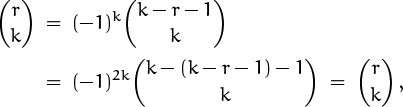
All these numbers are familiar. Indeed, the rows and columns of Table 164 appear as columns in Table 155 (but minus the minus signs). So there must be a connection between the values of for negative n and the values for positive n. The general rule is

it is easily proved, since

r^k = r(r – 1) . . . (r – k + 1)

= (–1)^k(–r)(1 – r) . . . (k – 1 – r) = (–1)^k(k – r – 1)^k

when k ≥ 0, and both sides are zero when k < 0.

Identity (5.14) is particularly valuable because it holds without any restriction. (Of course, the lower index must be an integer so that the binomial coefficients are defined.) The transformation in (5.14) is called negating the upper index, or “upper negation.”

But how can we remember this important formula? The other identities we’ve seen—symmetry, absorption, addition, etc.—are pretty simple, but this one looks rather messy. Still, there’s a mnemonic that’s not too bad: To negate the upper index, we begin by writing down (–1)^k, where k is the lower index. (The lower index doesn’t change.) Then we immediately write k again, twice, in both lower and upper index positions. Then we negate the original upper index by subtracting it from the new upper index. And we complete the job by subtracting 1 more (always subtracting, not adding, because this is a negation process).

You call this a mnemonic? I’d call it pneumatic—full of air. It does help me remember, though.

Let’s negate the upper index twice in succession, for practice. We get

(Now is a good time to do warmup exercise 4.)

so we’re right back where we started. This is probably not what the framers of the identity intended; but it’s reassuring to know that we haven’t gone astray.

It’s also frustrating, if we’re trying to get somewhere else.

Some applications of (5.14) are, of course, more useful than this. We can use upper negation, for example, to move quantities between upper and lower index positions. The identity has a symmetric formulation,

which holds because both sides are equal to .

Upper negation can also be used to derive the following interesting sum:

The idea is to negate the upper index, then apply (5.9), and negate again:

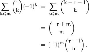
(Here double negation helps, because we’ve sandwiched another operation in between.)

This formula gives us a partial sum of the rth row of Pascal’s triangle, provided that the entries of the row have been given alternating signs. For instance, if r = 5 and m = 2 the formula gives .

Notice that if m ≥ r, (5.16) gives the alternating sum of the entire row, and this sum is zero when r is a positive integer. We proved this before, when we expanded (1 – 1)^r by the binomial theorem; it’s interesting to know that the partial sums of this expression can also be evaluated in closed form.

How about the simpler partial sum,

surely if we can evaluate the corresponding sum with alternating signs, we ought to be able to do this one? But no; there is no closed form for the partial sum of a row of Pascal’s triangle. We can do columns—that’s (5.10)—but not rows. Curiously, however, there is a way to partially sum the row elements if they have been multiplied by their distance from the center:

(This formula is easily verified by induction on m.) The relation between these partial sums with and without the factor of (r/2 – k) in the summand is analogous to the relation between the integrals

The apparently more complicated integral on the left, with the factor of x, has a closed form, while the simpler-looking integral on the right, without the factor, has none. Appearances can be deceiving.

(Well, the right-hand integral is , a constant plus a multiple of the “error function” of α, if we’re willing to accept that as a closed form.)

Near the end of this chapter, we’ll study a method by which it’s possible to determine whether or not there is a closed form for the partial sums of a given series involving binomial coefficients, in a fairly general setting. This method is capable of discovering identities (5.16) and (5.18), and it also will tell us that (5.17) is a dead end.

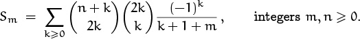
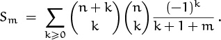
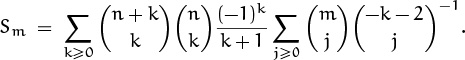
Partial sums of the binomial series lead to a curious relationship of another kind:

This identity isn’t hard to prove by induction: Both sides are zero when m < 0 and 1 when m = 0. If we let S_m stand for the sum on the left, we can apply the addition formula (5.8) and show easily that

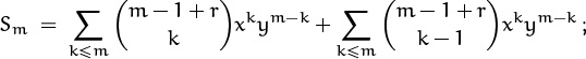
and

when m > 0. Hence

and this recurrence is satisfied also by the right-hand side of (5.19). By induction, both sides must be equal; QED.

But there’s a neater proof. When r is an integer in the range 0 ≥ r ≥ –m, the binomial theorem tells us that both sides of (5.19) are (x + y)^m+ry^–r. And since both sides are polynomials in r of degree m or less, agreement at m+1 different values is enough (but just barely!) to prove equality in general.

It may seem foolish to have an identity where one sum equals another. Neither side is in closed form. But sometimes one side turns out to be easier to evaluate than the other. For example, if we set x = –1 and y = 1, we get

an alternative form of identity (5.16). And if we set x = y = 1 and r = m + 1, we get

The left-hand side sums just half of the binomial coefficients with upper index 2m + 1, and these are equal to their counterparts in the other half because Pascal’s triangle has left-right symmetry. Hence the left-hand side is just . This yields a formula that is quite unexpected,

(There’s a nice combinatorial proof of this formula [247].)

Let’s check it when m = 2: . Astounding.

So far we’ve been looking either at binomial coefficients by themselves or at sums of terms in which there’s only one binomial coefficient per term. But many of the challenging problems we face involve products of two or more binomial coefficients, so we’ll spend the rest of this section considering how to deal with such cases.

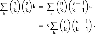
Here’s a handy rule that often helps to simplify the product of two binomial coefficients:

We’ve already seen the special case k = 1; it’s the absorption identity (5.6). Although both sides of (5.21) are products of binomial coefficients, one side often is easier to sum because of interactions with the rest of a formula. For example, the left side uses m twice, the right side uses it only once. Therefore we usually want to replace by when summing on m.

Equation (5.21) holds primarily because of cancellation between m!’s in the factorial representations of and . If all variables are integers and r ≥ m ≥ k ≥ 0, we have

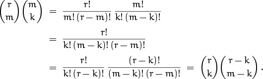
That was easy. Furthermore, if m < k or k < 0, both sides of (5.21) are zero; so the identity holds for all integers m and k. Finally, the polynomial argument extends its validity to all real r.

Yeah, right.

A binomial coefficient can be written in the form (a + b)!/a! b! after a suitable renaming of variables. Similarly, the quantity in the middle of the derivation above, r!/k! (m – k)! (r – m)!, can be written in the form (a + b + c)!/a! b! c!. This is a “trinomial coefficient,” which arises in the “trinomial theorem”:

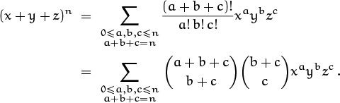
So is really a trinomial coefficient in disguise. Trinomial coefficients pop up occasionally in applications, and we can conveniently write them as

“Excogitavi autem olim mirabilem regulam pro numeris coefficientibus potestatum, non tantum a binomio x + y, sed et a trinomio x + y + z, imo a polynomio quocunque, ut data potentia gradus cujuscunque v. gr. decimi, et potentia in ejus valore comprehensa, ut x⁵ y³ z², possim statim assignare numerum coefficientem, quem habere debet, sine ulla Tabula jam calculata.”

—G. W. Leibniz [245]

in order to emphasize the symmetry present.

Binomial and trinomial coefficients generalize to multinomial coefficients, which are always expressible as products of binomial coefficients:

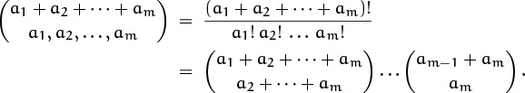
Therefore, when we run across such a beastie, our standard techniques apply.

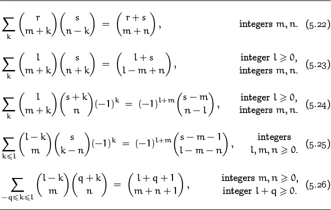
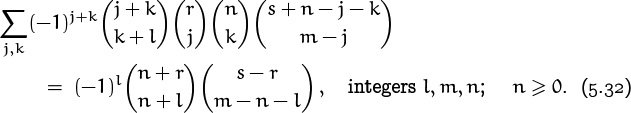
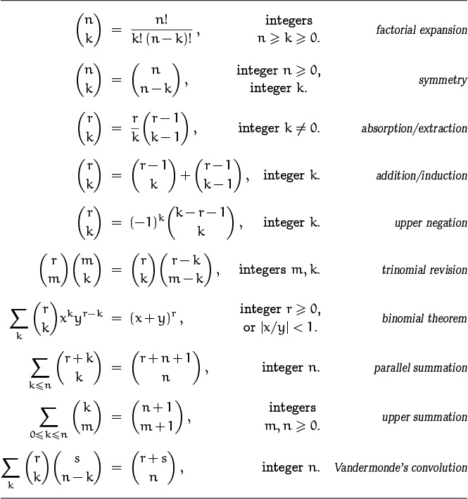
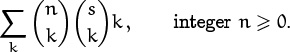
Now we come to Table 169, which lists identities that are among the most important of our standard techniques. These are the ones we rely on when struggling with a sum involving a product of two binomial coefficients. Each of these identities is a sum over k, with one appearance of k in each binomial coefficient; there also are four nearly independent parameters, called m, n, r, etc., one in each index position. Different cases arise depending on whether k appears in the upper or lower index, and on whether it appears with a plus or minus sign. Sometimes there’s an additional factor of (–1)^k, which is needed to make the terms summable in closed form.

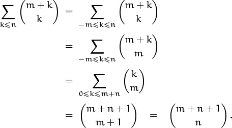
Table 169 is far too complicated to memorize in full; it is intended only for reference. But the first identity in this table is by far the most memorable, and it should be remembered. It states that the sum (over all integers k) of the product of two binomial coefficients, in which the upper indices are constant and the lower indices have a constant sum for all k, is the binomial coefficient obtained by summing both lower and upper indices. This identity is known as Vandermonde’s convolution, because Alexandre Vandermonde wrote a significant paper about it in the late 1700s [357]; it was, however, known to Chu Shih-Chieh in China as early as 1303. All of the other identities in Table 169 can be obtained from Vandermonde’s convolution by doing things like negating upper indices or applying the symmetry law, etc., with care; therefore Vandermonde’s convolution is the most basic of all.

Fold down the corner on this page, so you can find the table quickly later. You’ll need it!

We can prove Vandermonde’s convolution by giving it a nice combinatorial interpretation. If we replace k by k – m and n by n – m, we can assume that m = 0; hence the identity to be proved is

Let r and s be nonnegative integers; the general case then follows by the polynomial argument. On the right side, is the number of ways to choose n people from among r men and s women. On the left, each term of the sum is the number of ways to choose k of the men and n – k of the women. Summing over all k counts each possibility exactly once.

Sexist! You mentioned men first.

Much more often than not we use these identities left to right, since that’s the direction of simplification. But every once in a while it pays to go the other direction, temporarily making an expression more complicated. When this works, we’ve usually created a double sum for which we can interchange the order of summation and then simplify.

Before moving on let’s look at proofs for two more of the identities in Table 169. It’s easy to prove (5.23); all we need to do is replace the first binomial coefficient by , then Vandermonde’s (5.22) applies.

The next one, (5.24), is a bit more difficult. We can reduce it to Vandermonde’s convolution by a sequence of transformations, but we can just as easily prove it by resorting to the old reliable technique of mathematical induction. Induction is often the first thing to try when nothing else obvious jumps out at us, and induction on l works just fine here.

For the basis l = 0, all terms are zero except when k = –m; so both sides of the equation are . Now suppose that the identity holds for all values less than some fixed l, where l > 0. We can use the addition formula to replace by ; the original sum now breaks into two sums, each of which can be evaluated by the induction hypothesis:

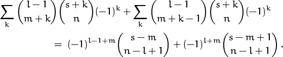
And this simplifies to the right-hand side of (5.24), if we apply the addition formula once again.

Two things about this derivation are worthy of note. First, we see again the great convenience of summing over all integers k, not just over a certain range, because there’s no need to fuss over boundary conditions. Second, the addition formula works nicely with mathematical induction, because it’s a recurrence for binomial coefficients. A binomial coefficient whose upper index is l is expressed in terms of two whose upper indices are l – 1, and that’s exactly what we need to apply the induction hypothesis.

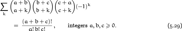
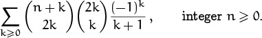
So much for Table 169. What about sums with three or more binomial coefficients? If the index of summation is spread over all the coefficients, our chances of finding a closed form aren’t great: Only a few closed forms are known for sums of this kind, hence the sum we need might not match the given specs. One of these rarities, proved in exercise 43, is

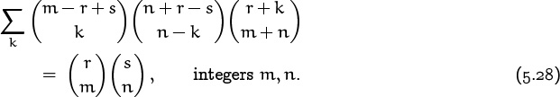
Here’s another, more symmetric example:

This one has a two-coefficient counterpart,

which incidentally doesn’t appear in Table 169. The analogous four-coefficient sum doesn’t have a closed form, but a similar sum does:

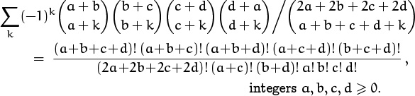
This follows from a five-parameter identity discovered by John Dougall [82] early in the twentieth century.

Is Dougall’s identity the hairiest sum of binomial coefficients known? No! The champion so far is

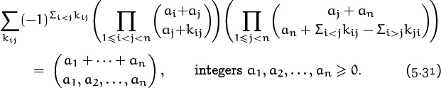
Here the sum is over index variables k_ij for 1 ≤ i < j < n. Equation (5.29) is the special case n = 3; the case n = 4 can be written out as follows, if we use (a, b, c, d) for (a₁, a₂, a₃, a₄) and (i, j, k) for (k₁₂, k₁₃, k₂₃):

The left side of (5.31) is the coefficient of after the product of n(n – 1) fractions

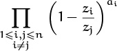
has been fully expanded into positive and negative powers of the z’s. The right side of (5.31) was conjectured by Freeman Dyson in 1962 and proved by several people shortly thereafter. Exercise 86 gives a “simple” proof of (5.31).

Another noteworthy identity involving lots of binomial coefficients is

This one, proved in exercise 83, even has a chance of arising in practical applications. But we’re getting far afield from our theme of “basic identities,” so we had better stop and take stock of what we’ve learned.

We’ve seen that binomial coefficients satisfy an almost bewildering variety of identities. Some of these, fortunately, are easily remembered, and we can use the memorable ones to derive most of the others in a few steps. Table 174 collects ten of the most useful formulas, all in one place; these are the best identities to know.

5.2 Basic Practice

In the previous section we derived a bunch of identities by manipulating sums and plugging in other identities. It wasn’t too tough to find those derivations—we knew what we were trying to prove, so we could formulate a general plan and fill in the details without much trouble. Usually, however, out in the real world, we’re not faced with an identity to prove; we’re faced with a sum to simplify. And we don’t know what a simplified form might look like (or even if one exists). By tackling many such sums in this section and the next, we will hone our binomial coefficient tools.

To start, let’s try our hand at a few sums involving a single binomial coefficient.

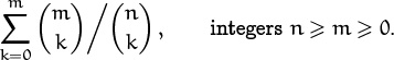
Problem 1: A sum of ratios.

We’d like to have a closed form for

Algorithm self-teach:
1 read problem
2 attempt solution
3 skim book solution
4 if attempt failed goto 1 else goto next problem

At first glance this sum evokes panic, because we haven’t seen any identities that deal with a quotient of binomial coefficients. (Furthermore the sum involves two binomial coefficients, which seems to contradict the sentence preceding this problem.) However, just as we can use the factorial representations to reexpress a product of binomial coefficients as another product—that’s how we got identity (5.21)—we can do likewise with a quotient. In fact we can avoid the grubby factorial representations by letting r = n and dividing both sides of equation (5.21) by ; this yields

Unfortunately, that algorithm can put you in an infinite loop.

Suggested patches:

0 set c ← 0
3a set c ← c + 1
3b if c = N
goto your TA

So we replace the quotient on the left, which appears in our sum, by the one on the right; the sum becomes

We still have a quotient, but the binomial coefficient in the denominator doesn’t involve the index of summation k, so we can remove it from the sum. We’ll restore it later.

—E. W. Dijkstra

We can also simplify the boundary conditions by summing over all k ≥ 0; the terms for k > m are zero. The sum that’s left isn’t so intimidating:

. . . But this sub-chapter is called BASIC practice.

It’s similar to the one in identity (5.9), because the index k appears twice with the same sign. But here it’s –k and in (5.9) it’s not. The next step should therefore be obvious; there’s only one reasonable thing to do:

And now we can apply the parallel summation identity, (5.9):

Finally we reinstate the in the denominator that we removed from the sum earlier, and then apply (5.7) to get the desired closed form:

This derivation actually works for any real value of n, as long as no division by zero occurs; that is, as long as n isn’t one of the integers 0, 1, . . . , m – 1.

The more complicated the derivation, the more important it is to check the answer. This one wasn’t too complicated but we’ll check anyway. In the small case m = 2 and n = 4 we have

yes, this agrees perfectly with our closed form (4 + 1)/(4 + 1 – 2).

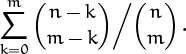
Problem 2: From the literature of sorting.

Our next sum appeared way back in ancient times (the early 1970s) before people were fluent with binomial coefficients. A paper that introduced an improved merging technique [196] concludes with the following remarks: “It can be shown that the expected number of saved transfers . . . is given by the expression

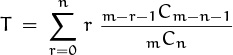
Here m and n are as defined above, and _m C_n is the symbol for the number of combinations of m objects taken n at a time. . . . The author is grateful to the referee for reducing a more complex equation for expected transfers saved to the form given here.”

We’ll see that this is definitely not a final answer to the author’s problem. It’s not even a midterm answer.

Please, don’t remind me of the midterm.

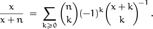
First we should translate the sum into something we can work with; the ghastly notation _m–r–1 C_m–n–1 is enough to stop anybody, save the enthusiastic referee (please). In our language we’d write

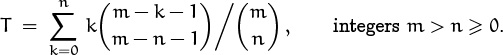
The binomial coefficient in the denominator doesn’t involve the index of summation, so we can remove it and work with the new sum

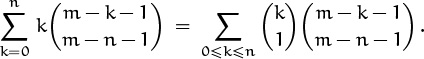
What next? The index of summation appears in the upper index of the binomial coefficient but not in the lower index. So if the other k weren’t there, we could massage the sum and apply summation on the upper index (5.10). With the extra k, though, we can’t. If we could somehow absorb that k into the binomial coefficient, using one of our absorption identities, we could then sum on the upper index. Unfortunately those identities don’t work here. But if the k were instead m – k, we could use absorption identity (5.6):

So here’s the key: We’ll rewrite k as m – (m – k) and split the sum S into two sums:

where

The sums A and B that remain are none other than our old friends in which the upper index varies while the lower index stays fixed. Let’s do B first, because it looks simpler. A little bit of massaging is enough to make the summand match the left side of (5.10):

In the last step we’ve included the terms with 0 ≤ k < m – n in the sum; they’re all zero, because the upper index is less than the lower. Now we sum on the upper index, using (5.10), and get

The other sum A is the same, but with m replaced by m – 1. Hence we have a closed form for the given sum S, which can be simplified further:

And this gives us a closed form for the original sum:

Even the referee can’t simplify this.

Again we use a small case to check the answer. When m = 4 and n = 2, we have

which agrees with our formula 2/(4 – 2 + 1).

Problem 3: From an old exam.

Let’s do one more sum that involves a single binomial coefficient. This one, unlike the last, originated in the halls of academia; it was a problem on a take-home test. We want the value of Q_1000000, when

Do old exams ever die?

This one’s harder than the others; we can’t apply any of the identities we’ve seen so far. And we’re faced with a sum of 2^1000000 + 1 terms, so we can’t just add them up. The index of summation k appears in both indices, upper and lower, but with opposite signs. Negating the upper index doesn’t help, either; it removes the factor of (–1)^k, but it introduces a 2k in the upper index.

When nothing obvious works, we know that it’s best to look at small cases. If we can’t spot a pattern and prove it by induction, at least we’ll have some data for checking our results. Here are the nonzero terms and their sums for the first four values of n.

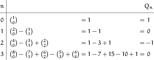
We’d better not try the next case, n = 4; the chances of making an arithmetic error are too high. (Computing terms like and by hand, let alone combining them with the others, is worthwhile only if we’re desperate.)

So the pattern starts out 1, 0, –1, 0. Even if we knew the next term or two, the closed form wouldn’t be obvious. But if we could find and prove a recurrence for Q_n we’d probably be able to guess and prove its closed form. To find a recurrence, we need to relate Q_n to Q_{n– 1} (or to Q_{smaller values}); but to do this we need to relate a term like , which arises when n = 7 and k = 13, to terms like . This doesn’t look promising; we don’t know any neat relations between entries in Pascal’s triangle that are 64 rows apart. The addition formula, our main tool for induction proofs, only relates entries that are one row apart.

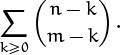
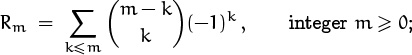
But this leads us to a key observation: There’s no need to deal with entries that are 2^n–1 rows apart. The variable n never appears by itself, it’s always in the context 2ⁿ. So the 2ⁿ is a red herring! If we replace 2ⁿ by m, all we need to do is find a closed form for the more general (but easier) sum

Oh, the sneakiness of the instructor who set that exam.

then we’ll also have a closed form for Q_n = R_2ⁿ. And there’s a good chance that the addition formula will give us a recurrence for the sequence R_m.

Values of R_m for small m can be read from Table 155, if we alternately add and subtract values that appear in a southwest-to-northeast diagonal. The results are:

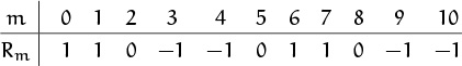
There seems to be a lot of cancellation going on.

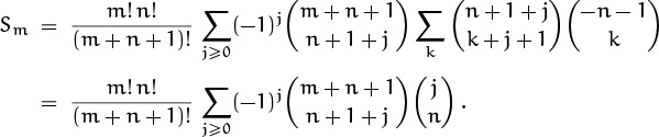
Let’s look now at the formula for R_m and see if it defines a recurrence. Our strategy is to apply the addition formula (5.8) and to find sums that have the form R_k in the resulting expression, somewhat as we did in the perturbation method of Chapter 2:

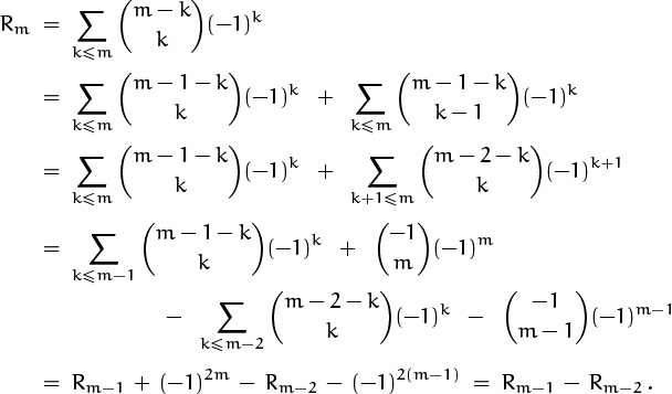
(In the next-to-last step we’ve used the formula , which we know is true when m ≥ 0.) This derivation is valid for m ≥ 2.

Anyway those of us who’ve done warmup exercise 4 know it.

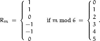
From this recurrence we can generate values of R_m quickly, and we soon perceive that the sequence is periodic. Indeed,

The proof by induction is by inspection. Or, if we must give a more academic proof, we can unfold the recurrence one step to obtain

R_m = (R_m–2 – R_m–3) – R_m–2 = –R_m–3 ,

whenever m ≥ 3. Hence R_m = R_m–6 whenever m ≥ 6.

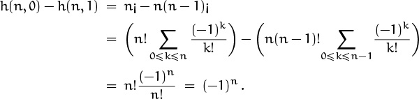
Finally, since Q_n = R_2ⁿ, we can determine Q_n by determining 2ⁿ mod 6 and using the closed form for R_m. When n = 0 we have 2⁰ mod 6 = 1; after that we keep multiplying by 2 (mod 6), so the pattern 2, 4 repeats. Thus

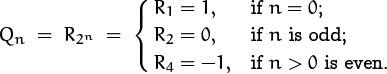
This closed form for Q_n agrees with the first four values we calculated when we started on the problem. We conclude that Q_1000000 = R₄ = –1.

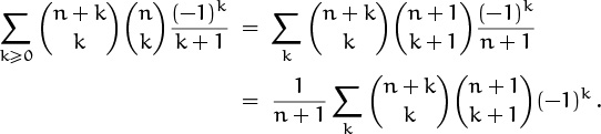
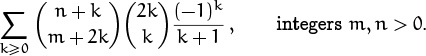
Problem 4: A sum involving two binomial coefficients.

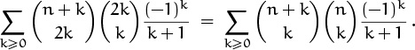
Our next task is to find a closed form for

Wait a minute. Where’s the second binomial coefficient promised in the title of this problem? And why should we try to simplify a sum we’ve already simplified? (This is the sum S from Problem 2.)

Well, this is a sum that’s easier to simplify if we view the summand as a product of two binomial coefficients, and then use one of the general identities found in Table 169. The second binomial coefficient materializes when we rewrite k as :

And identity (5.26) is the one to apply, since its index of summation appears in both upper indices and with opposite signs.

But our sum isn’t quite in the correct form yet. The upper limit of summation should be m – 1, if we’re to have a perfect match with (5.26). No problem; the terms for n < k ≤ m – 1 are zero. So we can plug in, with (l, m, n, q) ← (m – 1, m – n – 1, 1, 0); the answer is

This is cleaner than the formula we got before. We can convert it to the previous formula by using (5.6) and (5.7):

Similarly, we can get interesting results by plugging special values into the other general identities we’ve seen. Suppose, for example, that we set m = n = 1 and q = 0 in (5.26). Then the identity reads

The left side is l ((l + 1)l/2) – (1² + 2² + · · · + l²), so this gives us a brand new way to solve the sum-of-squares problem that we beat to death in Chapter 2.

The moral of this story is: Special cases of very general sums are sometimes best handled in the general form. When learning general forms, it’s wise to learn their simple specializations.

Problem 5: A sum with three factors.

Here’s another sum that isn’t too bad. We wish to simplify

The index of summation k appears in both lower indices and with the same sign; therefore identity (5.23) in Table 169 looks close to what we need. With a bit of manipulation, we should be able to use it.

The biggest difference between (5.23) and what we have is the extra k in our sum. But we can absorb k into one of the binomial coefficients by using one of the absorption identities:

We don’t care that the s appears when the k disappears, because it’s constant. And now we’re ready to apply the identity and get the closed form,

If we had chosen in the first step to absorb k into , not , we wouldn’t have been allowed to apply (5.23) directly, because n – 1 might be negative; the identity requires a nonnegative value in at least one of the upper indices.

Problem 6: A sum with menacing characteristics.

The next sum is more challenging. We seek a closed form for

So we should deep six this sum, right?

One useful measure of a sum’s difficulty is the number of times the index of summation appears. By this measure we’re in deep trouble—k appears six times. Furthermore, the key step that worked in the previous problem—to absorb something outside the binomial coefficients into one of them—won’t work here. If we absorb the k + 1 we just get another occurrence of k in its place. And not only that: Our index k is twice shackled with the coefficient 2 inside a binomial coefficient. Multiplicative constants are usually harder to remove than additive constants.

We’re lucky this time, though. The 2k’s are right where we need them for identity (5.21) to apply, so we get

The two 2’s disappear, and so does one occurrence of k. So that’s one down and five to go.

The k + 1 in the denominator is the most troublesome characteristic left, and now we can absorb it into using identity (5.5):

(Recall that n ≥ 0.) Two down, four to go.

To eliminate another k we have two promising options. We could use symmetry on ; or we could negate the upper index n + k, thereby eliminating that k as well as the factor (–1)^k. Let’s explore both possibilities, starting with the symmetry option:

Third down, three to go, and we’re in position to make a big gain by plugging into (5.24): Replacing (l, m, n, s) by (n + 1, 1, n, n), we get

For a minute I thought we’d have to punt.

Zero, eh? After all that work? Let’s check it when n = 2: . It checks.

Just for the heck of it, let’s explore our other option, negating the upper index of :

Now (5.23) applies, with (l, m, n, s) ← (n + 1, 1, 0, –n – 1), and

Hey wait. This is zero when n > 0, but it’s 1 when n = 0. Our other path to the solution told us that the sum was zero in all cases! What gives? The sum actually does turn out to be 1 when n = 0, so the correct answer is ‘[n = 0]’. We must have made a mistake in the previous derivation.

Let’s do an instant replay on that derivation when n = 0, in order to see where the discrepancy first arises. Ah yes; we fell into the old trap mentioned earlier: We tried to apply symmetry when the upper index could be negative! We were not justified in replacing by when k ranges over all integers, because this converts zero into a nonzero value when k < –n. (Sorry about that.)

Try binary search: Replay the middle formula first, to see if the mistake was early or late.

The other factor in the sum, , turns out to be zero when k < –n, except when n = 0 and k = –1. Hence our error didn’t show up when we checked the case n = 2. Exercise 6 explains what we should have done.

Problem 7: A new obstacle.

This one’s even tougher; we want a closed form for

If m were 0 we’d have the sum from the problem we just finished. But it’s not, and we’re left with a real mess—nothing we used in Problem 6 works here. (Especially not the crucial first step.)

However, if we could somehow get rid of the m, we could use the result just derived. So our strategy is: Replace by a sum of terms like for some nonnegative integer l; the summand will then look like the summand in Problem 6, and we can interchange the order of summation.

What should we substitute for ? A painstaking examination of the identities derived earlier in this chapter turns up only one suitable candidate, namely equation (5.26) in Table 169. And one way to use it is to replace the parameters (l, m, n, q, k) by (n + k – 1, 2k, m – 1, 0, j), respectively:

In the last step we’ve changed the order of summation, manipulating the conditions below the ∑’s according to the rules of Chapter 2.

We can’t quite replace the inner sum using the result of Problem 6, because it has the extra condition k ≥ j – n + 1. But this extra condition is superfluous unless j – n + 1 > 0; that is, unless j ≥ n. And when j ≥ n, the first binomial coefficient of the inner sum is zero, because its upper index is between 0 and k – 1, thus strictly less than the lower index 2k. We may therefore place the additional restriction j < n on the outer sum, without affecting which nonzero terms are included. This makes the restriction k ≥ j – n + 1 superfluous, and we can use the result of Problem 6. The double sum now comes tumbling down:

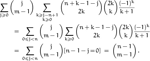
The inner sums vanish except when j = n – 1, so we get a simple closed form as our answer.

Problem 8: A different obstacle.

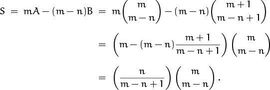
Let’s branch out from Problem 6 in another way by considering the sum

Again, when m = 0 we have the sum we did before; but now the m occurs in a different place. This problem is a bit harder yet than Problem 7, but (fortunately) we’re getting better at finding solutions. We can begin as in Problem 6,

Now (as in Problem 7) we try to expand the part that depends on m into terms that we know how to deal with. When m was zero, we absorbed k + 1 into ; if m > 0, we can do the same thing if we expand 1/(k + 1 + m) into absorbable terms. And our luck still holds: We proved a suitable identity

in Problem 1. Replacing r by –k – 2 gives the desired expansion,

Now the (k + 1)^–1 can be absorbed into , as planned. In fact, it could also be absorbed into . Double absorption suggests that even more cancellation might be possible behind the scenes. Yes—expanding everything in our new summand into factorials and going back to binomial coefficients gives a formula that we can sum on k:

They expect us to check this on a sheet of scratch paper.

The sum over all integers j is zero, by (5.24). Hence –S_m is the sum for j < 0.

To evaluate –S_m for j < 0, let’s replace j by –k – 1 and sum for k ≥ 0:

Finally (5.25) applies, and we have our answer:

Whew; we’d better check it. When n = 2 we find

Our derivation requires m to be an integer, but the result holds for all real m, because the quantity is a polynomial in m of degree ≤ n.

5.3 Tricks of the Trade

Let’s look next at three techniques that significantly amplify the methods we have already learned.

Trick 1: Going halves.

Many of our identities involve an arbitrary real number r. When r has the special form “integer minus one half,” the binomial coefficient can be written as a quite different-looking product of binomial coefficients. This leads to a new family of identities that can be manipulated with surprising ease.

This should really be called Trick 1/2.

One way to see how this works is to begin with the duplication formula

This identity is obvious if we expand the falling powers and interleave the factors on the left side:

Now we can divide both sides by k!², and we get

If we set k = r = n, where n is an integer, this yields

And negating the upper index gives yet another useful formula,

For example, when n = 4 we have

. . . we halve . . .

Notice how we’ve changed a product of odd numbers into a factorial.

Identity (5.35) has an amusing corollary. Let , and take the sum over all integers k. The result is

by (5.23), because either n/2 or (n – 1)/2 is n/2, a nonnegative integer!

We can also use Vandermonde’s convolution (5.27) to deduce that

Plugging in the values from (5.37) gives

this is what sums to (–1)ⁿ. Hence we have a remarkable property of the “middle” elements of Pascal’s triangle:

For example, .

These illustrations of our first trick indicate that it’s wise to try changing binomial coefficients of the form into binomial coefficients of the form , where n is some appropriate integer (usually 0, 1, or k); the resulting formula might be much simpler.

Trick 2: High-order differences.

We saw earlier that it’s possible to evaluate partial sums of the series , but not of the series . It turns out that there are many important applications of binomial coefficients with alternating signs, . One of the reasons for this is that such coefficients are intimately associated with the difference operator Δ defined in Section 2.6.

The difference Δf of a function f at the point x is

Δf(x) = f(x + 1) – f(x);

if we apply Δ again, we get the second difference

Δ2 f(x) = Δf(x + 1) – Δf(x)	= (f(x + 2) – f(x + 1)) – (f(x+1) – f(x))
	= f(x + 2) – 2f(x + 1) + f(x),

which is analogous to the second derivative. Similarly, we have

Δ³ f(x) = f(x + 3) – 3f(x + 2) + 3f(x + 1) – f(x);

Δ⁴ f(x) = f(x + 4) – 4f(x + 3) + 6f(x + 2) – 4f(x + 1) + f(x);

and so on. Binomial coefficients enter these formulas with alternating signs.

In general, the nth difference is

This formula is easily proved by induction, but there’s also a nice way to prove it directly using the elementary theory of operators. Recall that Section 2.6 defines the shift operator E by the rule

Ef(x) = f(x + 1);

hence the operator Δ is E – 1, where 1 is the identity operator defined by the rule 1f(x) = f(x). By the binomial theorem,

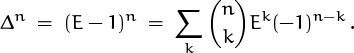
This is an equation whose elements are operators; it is equivalent to (5.40), since E^k is the operator that takes f(x) into f(x + k).

An interesting and important case arises when we consider negative falling powers. Let . Then, by rule (2.45), we have , , and in general

Equation (5.40) now tells us that

For example,

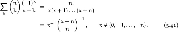
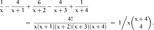
The sum in (5.41) is the partial fraction expansion of n!/(x(x + 1) . . . (x + n)).

Significant results can be obtained from positive falling powers too. If f(x) is a polynomial of degree d, the difference Δf(x) is a polynomial of degree d–1; therefore Δ^d f(x) is a constant, and Δⁿ f(x) = 0 if n > d. This extremely important fact simplifies many formulas.

A closer look gives further information: Let

f(x) = a_dx^d + a_d–1x^d–1 + · · · + a₁x¹ + a₀x⁰

be any polynomial of degree d. We will see in Chapter 6 that we can express ordinary powers as sums of falling powers (for example, x² = x² + x¹); hence there are coefficients b_d, b_d–1, . . . , b₁, b₀ such that

f(x) = b_dx^d + b_d–1x^d–1 + · · · + b₁x¹ + b₀x⁰ .

(It turns out that b_d = a_d and b₀ = a₀, but the intervening coefficients are related in a more complicated way.) Let c_k = k! b_k for 0 ≤ k ≤ d. Then

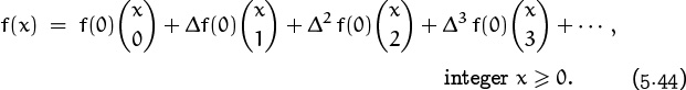
thus, any polynomial can be represented as a sum of multiples of binomial coefficients. Such an expansion is called the Newton series of f(x), because Isaac Newton used it extensively.

We observed earlier in this chapter that the addition formula implies

Therefore, by induction, the nth difference of a Newton series is very simple:

If we now set x = 0, all terms on the right side are zero, except the term with k – n = 0; hence

The Newton series for f(x) is therefore

For example, suppose f(x) = x³. It’s easy to calculate

f(0) = 0,        f(1) = 1,        f(2) = 8,        f(3) = 27;

Δf(0) = 1,        Δf(1) = 7,        Δf(2) = 19;

Δ² f(0) = 6,        Δ² f(1) = 12;

Δ³ f(0) = 6.

So the Newton series is .

Our formula Δⁿ f(0) = c_n can also be stated in the following way, using (5.40) with x = 0:

Here c₀, c₁, c₂, . . . is an arbitrary sequence of coefficients; the infinite sum is actually finite for all k ≥ 0, so convergence is not an issue. In particular, we can prove the important identity

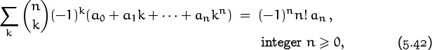
because the polynomial a₀ + a₁k + · · · + a_nkⁿ can always be written as a Newton series with c_n = n! a_n.

Many sums that appear to be hopeless at first glance can actually be summed almost trivially by using the idea of nth differences. For example, let’s consider the identity

This looks very impressive, because it’s quite different from anything we’ve seen so far. But it really is easy to understand, once we notice the telltale factor in the summand, because the function

is a polynomial in k of degree n, with leading coefficient (–1)ⁿsⁿ/n!. Therefore (5.43) is nothing more than an application of (5.42).

We have discussed Newton series under the assumption that f(x) is a polynomial. But we’ve also seen that infinite Newton series

make sense too, because such sums are always finite when x is a nonnegative integer. Our derivation of the formula Δⁿ f(0) = c_n works in the infinite case, just as in the polynomial case; so we have the general identity

This formula is valid for any function f(x) that is defined for nonnegative integers x. Moreover, if the right-hand side converges for other values of x, it defines a function that “interpolates” f(x) in a natural way. (There are infinitely many ways to interpolate function values, so we cannot assert that (5.44) is true for all x that make the infinite series converge. For example, if we let f(x) = sin(πx), we have f(x) = 0 at all integer points, so the right-hand side of (5.44) is identically zero; but the left-hand side is nonzero at all noninteger x.)

A Newton series is finite calculus’s answer to infinite calculus’s Taylor series. Just as a Taylor series can be written

the Newton series for f(x) = g(a + x) can be written

(Since E = 1 + Δ, ; and E^xg(a) = g(a + x).)

(This is the same as (5.44), because Δⁿ f(0) = Δⁿ g(a) for all n ≥ 0 when f(x) = g(a + x).) Both the Taylor and Newton series are finite when g is a polynomial, or when x = 0; in addition, the Newton series is finite when x is a positive integer. Otherwise the sums may or may not converge for particular values of x. If the Newton series converges when x is not a nonnegative integer, it might actually converge to a value that’s different from g(a + x), because the Newton series (5.45) depends only on the spaced-out function values g(a), g(a + 1), g(a + 2), . . . .

One example of a convergent Newton series is provided by the binomial theorem. Let g(x) = (1 + z)^x, where z is a fixed complex number such that |z| < 1. Then Δg(x) = (1 + z)^x+1 – (1 + z)^x = z(1 + z)^x, hence Δⁿ g(x) = zⁿ(1 + z)^x. In this case the infinite Newton series

converges to the “correct” value (1 + z)^a+x, for all x.

James Stirling tried to use Newton series to generalize the factorial function to noninteger values. First he found coefficients S_n such that

is an identity for x = 0, x = 1, x = 2, etc. But he discovered that the resulting series doesn’t converge except when x is a nonnegative integer. So he tried again, this time writing

“Forasmuch as these terms increase very fast, their differences will make a diverging progression, which hinders the ordinate of the parabola from approaching to the truth; therefore in this and the like cases, I interpolate the logarithms of the terms, whose differences constitute a series swiftly converging.”

—J. Stirling [343]

Now Δ(ln x!) = ln(x + 1)! – ln x! = ln(x + 1), hence

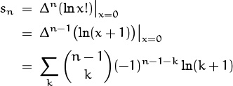
by (5.40). The coefficients are therefore s₀ = s₁ = 0; s₂ = ln 2; ; ; etc. In this way Stirling obtained a series that does converge (although he didn’t prove it); in fact, his series converges for all x > –1. He was thereby able to evaluate ! satisfactorily. Exercise 88 tells the rest of the story.

(Proofs of convergence were not invented until the nineteenth century.)

Trick 3: Inversion.

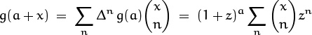
A special case of the rule (5.44) we’ve just derived for Newton’s series can be rewritten in the following way using (5.40):

This dual relationship between f and g is called an inversion formula; it’s rather like the Möbius inversion formulas (4.56) and (4.61) that we encountered in Chapter 4. Inversion formulas tell us how to solve “implicit recurrences,” where an unknown sequence is embedded in a sum.

Invert this: ‘zınb ppo’.

For example, g(n) might be a known function, and f(n) might be unknown; and we might have found a way to show that . Then (5.48) lets us express f(n) as a sum of known values.

We can prove (5.48) directly by using the basic methods at the beginning of this chapter. If for all n ≥ 0, then

The proof in the other direction is, of course, the same, because the relation between f and g is symmetric.

Let’s illustrate (5.48) by applying it to the “football victory problem”: A group of n fans of the winning football team throw their hats high into the air. The hats come back randomly, one hat to each of the n fans. How many ways h(n, k) are there for exactly k fans to get their own hats back?

For example, if n = 4 and if the hats and fans are named A, B, C, D, the 4! = 24 possible ways for hats to land generate the following numbers of rightful owners:

ABCD   4        BACD   2        CABD   1        DABC   0
ABDC   2        BADC   0        CADB   0        DACB   1
ACBD   2        BCAD   1        CBAD   2        DBAC   1
ACDB   1        BCDA   0        CBDA   1        DBCA   2
ADBC   1        BDAC   0        CDAB   0        DCAB   0
ADCB   2        BDCA   1        CDBA   0        DCBA   0

Therefore h(4, 4) = 1; h(4, 3) = 0; h(4, 2) = 6; h(4, 1) = 8; h(4, 0) = 9.

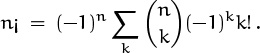
We can determine h(n, k) by noticing that it is the number of ways to choose k lucky hat owners, namely , times the number of ways to arrange the remaining n–k hats so that none of them goes to the right owner, namely h(n – k, 0). A permutation is called a derangement if it moves every item, and the number of derangements of n objects is sometimes denoted by the symbol ‘n¡’, read “n subfactorial.” Therefore h(n – k, 0) = (n – k)¡, and we have the general formula

(Subfactorial notation isn’t standard, and it’s not clearly a great idea; but let’s try it a while to see if we grow to like it. We can always resort to ‘D_n’ or something, if ‘n¡’ doesn’t work out.)

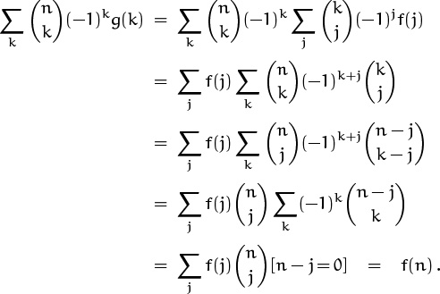
Our problem would be solved if we had a closed form for n¡, so let’s see what we can find. There’s an easy way to get a recurrence, because the sum of h(n, k) for all k is the total number of permutations of n hats:

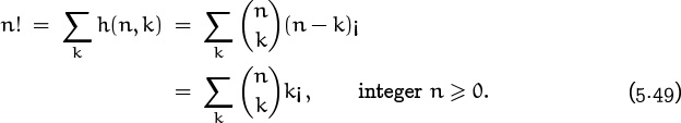
(We’ve changed k to n – k and to in the last step.) With this implicit recurrence we can compute all the h(n, k)’s we like:

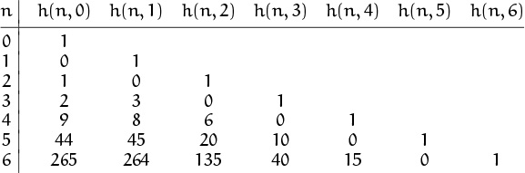
For example, here’s how the row for n = 4 can be computed: The two rightmost entries are obvious—there’s just one way for all hats to land correctly, and there’s no way for just three fans to get their own. (Whose hat would the fourth fan get?) When k = 2 and k = 1, we can use our equation for h(n, k), giving , and . We can’t use this equation for h(4, 0); rather, we can, but it gives us , which is true but useless. Taking another tack, we can use the relation h(4, 0) + 8 + 6 + 0 + 1 = 4! to deduce that h(4, 0) = 9; this is the value of 4¡. Similarly n¡ depends on the values of k¡ for k < n.

The art of mathematics, as of life, is knowing which truths are useless.

How can we solve a recurrence like (5.49)? Easy; it has the form of (5.48), with g(n) = n! and f(k) = (–1)^kk¡. Hence its solution is

Well, this isn’t really a solution; it’s a sum that should be put into closed form if possible. But it’s better than a recurrence. The sum can be simplified, since k! cancels with a hidden k! in , so let’s try that: We get

The remaining sum converges rapidly to the number . In fact, the terms that are excluded from the sum are

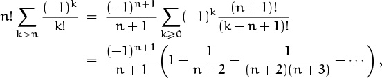
and the parenthesized quantity lies between 1 and . Therefore the difference between n¡ and n!/e is roughly 1/n in absolute value; more precisely, it lies between 1/(n + 1) and 1/(n + 2). But n¡ is an integer. Therefore it must be what we get when we round n!/e to the nearest integer, if n > 0. So we have the closed form we seek:

This is the number of ways that no fan gets the right hat back. When n is large, it’s more meaningful to know the probability that this happens. If we assume that each of the n! arrangements is equally likely—because the hats were thrown extremely high—this probability is

Baseball fans: .367 is also Ty Cobb’s lifetime batting average, the all-time record. Can this be a coincidence?

(Hey wait, you’re fudging. Cobb’s average was 4191/11429 ≈ .366699, while 1/e ≈ .367879. But maybe if Wade Boggs has a few really good seasons. . . )

So when n gets large the probability that all hats are misplaced is almost 37%.

Incidentally, recurrence (5.49) for subfactorials is exactly the same as (5.46), the first recurrence considered by Stirling when he was trying to generalize the factorial function. Hence S_k = k¡. These coefficients are so large, it’s no wonder the infinite series (5.46) diverges for noninteger x.

Before leaving this problem, let’s look briefly at two interesting patterns that leap out at us in the table of small h(n, k). First, it seems that the numbers 1, 3, 6, 10, 15, . . . below the all-0 diagonal are the triangular numbers. This observation is easy to prove, since those table entries are the h(n, n–2)’s, and we have

It also seems that the numbers in the first two columns differ by ±1. Is this always true? Yes,

In other words, n¡ = n(n – 1)¡ + (–1)ⁿ. This is a much simpler recurrence for the derangement numbers than we had before.

Now let’s invert something else. If we apply inversion to the formula

But inversion is the source of smog.

that we derived in (5.41), we find

This is interesting, but not really new. If we negate the upper index in , we have merely discovered identity (5.33) again.

5.4 Generating Functions

We come now to the most important idea in this whole book, the notion of a generating function. An infinite sequence a₀, a₁, a₂, . . . that we wish to deal with in some way can conveniently be represented as a power series in an auxiliary variable z,

It’s appropriate to use the letter z as the name of the auxiliary variable, because we’ll often be thinking of z as a complex number. The theory of complex variables conventionally uses ‘z’ in its formulas; power series (a.k.a. analytic functions or holomorphic functions) are central to that theory.

We will be seeing lots of generating functions in subsequent chapters. Indeed, Chapter 7 is entirely devoted to them. Our present goal is simply to introduce the basic concepts, and to demonstrate the relevance of generating functions to the study of binomial coefficients.

A generating function is useful because it’s a single quantity that represents an entire infinite sequence. We can often solve problems by first setting up one or more generating functions, then by fooling around with those functions until we know a lot about them, and finally by looking again at the coefficients. With a little bit of luck, we’ll know enough about the function to understand what we need to know about its coefficients.

If A(z) is any power series Σ_k≥0 a_kz^k, we will find it convenient to write

(See [223] for a discussion of the history and usefulness of this notation.)

in other words, [zⁿ] A(z) denotes the coefficient of zⁿ in A(z).

Let A(z) be the generating function for a₀, a₁, a₂, . . . as in (5.52), and let B(z) be the generating function for another sequence b₀, b₁, b₂, . . . . Then the product A(z)B(z) is the power series

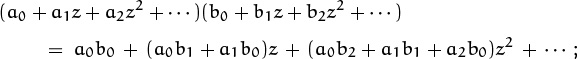
the coefficient of zⁿ in this product is

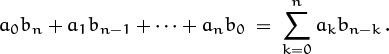
Therefore if we wish to evaluate any sum that has the general form

and if we know the generating functions A(z) and B(z), we have

c_n = [zⁿ] A(z)B(z) .

The sequence c_n defined by (5.54) is called the convolution of the sequences a_n and b_n; two sequences are “convolved” by forming the sums of all products whose subscripts add up to a given amount. The gist of the previous paragraph is that convolution of sequences corresponds to multiplication of their generating functions.

Generating functions give us powerful ways to discover and/or prove identities. For example, the binomial theorem tells us that (1 + z)^r is the generating function for the sequence :

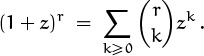
Similarly,

If we multiply these together, we get another generating function:

(1 + z)^r(1 + z)^s = (1 + z)^r+s .

And now comes the punch line: Equating coefficients of zⁿ on both sides of this equation gives us

We’ve discovered Vandermonde’s convolution, (5.27)!

(5.27)! = (5.27)(4.27)(3.27)(2.27)(1.27)(0.27)!.

That was nice and easy; let’s try another. This time we use (1–z)^r, which is the generating function for the sequence . Multiplying by (1 + z)^r gives another generating function whose coefficients we know:

(1 – z)^r(1 + z)^r = (1 – z²)^r .

Equating coefficients of zⁿ now gives the equation

We should check this on a small case or two. When n = 3, for example, the result is

Each positive term is cancelled by a corresponding negative term. And the same thing happens whenever n is odd, in which case the sum isn’t very interesting. But when n is even, say n = 2, we get a nontrivial sum that’s different from Vandermonde’s convolution:

So (5.55) checks out fine when n = 2. It turns out that (5.30) is a special case of our new identity (5.55).

Binomial coefficients also show up in some other generating functions, most notably the following important identities in which the lower index stays fixed and the upper index varies:

If you have a highlighter pen, these two equations have got to be marked.

The second identity here is just the first one multiplied by zⁿ, that is, “shifted right” by n places. The first identity is just a special case of the binomial theorem in slight disguise: If we expand (1 – z)^–n–1 by (5.13), the coefficient of z^k is , which can be rewritten as or by negating the upper index. These special cases are worth noting explicitly, because they arise so frequently in applications.

When n = 0 we get a special case of a special case, the geometric series:

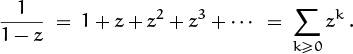
This is the generating function for the sequence 1, 1, 1, . . . , and it is especially useful because the convolution of any other sequence with this one is the sequence of sums: When b_k = 1 for all k, (5.54) reduces to

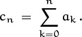
Therefore if A(z) is the generating function for the summands a₀, a₁, a₂, . . . , then A(z)/(1 – z) is the generating function for the sums c₀, c₁, c₂, . . . .

The problem of derangements, which we solved by inversion in connection with hats and football fans, can be resolved with generating functions in an interesting way. The basic recurrence

can be put into the form of a convolution if we expand in factorials and divide both sides by n!:

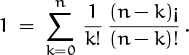
The generating function for the sequence is e^z; hence if we let

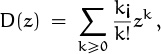
the convolution/recurrence tells us that

Solving for D(z) gives

Equating coefficients of zⁿ now tells us that

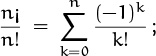
this is the formula we derived earlier by inversion.

So far our explorations with generating functions have given us slick proofs of things that we already knew how to derive by more cumbersome methods. But we haven’t used generating functions to obtain any new results, except for (5.55). Now we’re ready for something new and more surprising. There are two families of power series that generate an especially rich class of binomial coefficient identities: Let us define the generalized binomial series _t(z) and the generalized exponential series _t(z) as follows:

We will prove in Section 7.5 that these functions satisfy the identities

In the special case t = 0, we have

₀(z) = 1 + z ;                    ₀(z) = e^z ;

this explains why the series with parameter t are called “generalized” binomials and exponentials.

The following pairs of identities are valid for all real r:

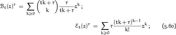
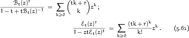
The generalized binomial series _t(z) was discovered in the 1750s by J. H. Lambert [236, §38], who noticed a few years later [237] that its powers satisfy the first identity in (5.60). Exercise 84 explains how to derive (5.61) from (5.60).

(When tk + r = 0, we have to be a little careful about how the coefficient of z^k is interpreted; each coefficient is a polynomial in r. For example, the constant term of _t(z)^r is r(0 + r)^–1, and this is equal to 1 even when r = 0.)

Since equations (5.60) and (5.61) hold for all r, we get very general identities when we multiply together the series that correspond to different powers r and s. For example,

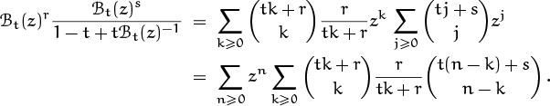
This power series must equal

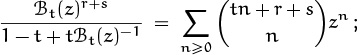
News flash:
ln  ;
ln  .

hence we can equate coefficients of zⁿ and get the identity

valid for all real r, s, and t. When t = 0 this identity reduces to Vandermonde’s convolution. (If by chance tk + r happens to equal zero in this formula, the denominator factor tk + r should be considered to cancel with the tk + r in the numerator of the binomial coefficient. Both sides of the identity are polynomials in r, s, and t.) Similar identities hold when we multiply _t(z)^r by _t(z)^s, etc.; Table 202 presents the results.

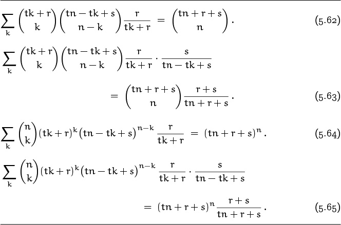
We have learned that it’s generally a good idea to look at special cases of general results. What happens, for example, if we set t = 1? The generalized binomial ₁(z) is very simple—it’s just

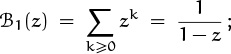
therefore ₁(z) doesn’t give us anything we didn’t already know from Vandermonde’s convolution. But ₁(z) is an important function,

which we haven’t seen before; it satisfies the basic identity

Aha! This is the iterated power function that I’ve often wondered about.

This function, first studied by Euler [117] and Eisenstein [91], arises in a great many applications [193, 204].

The special cases t = 2 and t = –1 of the generalized binomial are of particular interest, because their coefficients occur again and again in problems that have a recursive structure. Therefore it’s useful to display these series explicitly for future reference:

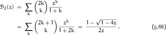
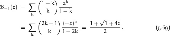
The power series for is noteworthy too.

The coefficients of ₂(z) are called the Catalan numbers C_n, because Eugène Catalan wrote an influential paper about them in the 1830s [52]. The sequence begins as follows:

The coefficients of _–1(z) are essentially the same, but there’s an extra 1 at the beginning and the other numbers alternate in sign: 1, 1, –1, 2, –5, 14, . . . . Thus _–1(z) = 1 + z₂(–z). We also have _–1(z) = ₂(–z)^–1.

Let’s close this section by deriving an important consequence of (5.72) and (5.73), a relation that shows further connections between the functions _–1(z) and ₂(–z):

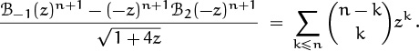
This holds because the coefficient of z^k in is

when k > n. The terms nicely cancel each other out. We can now use (5.68) and (5.69) to obtain the closed form

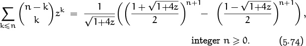
(The special case z = –1 came up in Problem 3 of Section 5.2. Since the numbers are sixth roots of unity, the sums have the periodic behavior we observed in that problem.) Similarly we can combine (5.70) with (5.71) to cancel the large coefficients and get

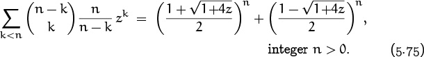
5.5 Hypergeometric Functions

The methods we’ve been applying to binomial coefficients are very effective, when they work, but we must admit that they often appear to be ad hoc—more like tricks than techniques. When we’re working on a problem, we often have many directions to pursue, and we might find ourselves going around in circles. Binomial coefficients are like chameleons, changing their appearance easily. Therefore it’s natural to ask if there isn’t some unifying principle that will systematically handle a great variety of binomial coefficient summations all at once. Fortunately, the answer is yes. The unifying principle is based on the theory of certain infinite sums called hypergeometric series.

They’re even more versatile than chameleons; we can dissect them and put them back together in different ways.

The study of hypergeometric series was launched many years ago by Euler, Gauss, and Riemann; such series, in fact, are still the subject of considerable research. But hypergeometrics have a somewhat formidable notation, which takes a little time to get used to.

Anything that has survived for centuries with such awesome notation must be really useful.

The general hypergeometric series is a power series in z with m + n parameters, and it is defined as follows in terms of rising factorial powers:

To avoid division by zero, none of the b’s may be zero or a negative integer. Other than that, the a’s and b’s may be anything we like. The notation ‘F(a₁, . . . , a_m; b₁, . . . , b_n; z)’ is also used as an alternative to the two-line form (5.76), since a one-line form sometimes works better typographically. The a’s are said to be upper parameters; they occur in the numerator of the terms of F. The b’s are lower parameters, and they occur in the denominator. The final quantity z is called the argument.

Standard reference books often use ‘_mF_n’ instead of ‘F’ as the name of a hypergeometric with m upper parameters and n lower parameters. But the extra subscripts tend to clutter up the formulas and waste our time, if we’re compelled to write them over and over. We can count how many parameters there are, so we usually don’t need extra additional unnecessary redundancy.

Many important functions occur as special cases of the general hypergeometric; indeed, that’s why hypergeometrics are so powerful. For example, the simplest case occurs when m = n = 0: There are no parameters at all, and we get the familiar series

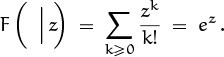
Actually the notation looks a bit unsettling when m or n is zero. We can add an extra ‘1’ above and below in order to avoid this:

In general we don’t change the function if we cancel a parameter that occurs in both numerator and denominator, or if we insert two identical parameters.

The next simplest case has m = 1, a₁ = 1, and n = 0; we change the parameters to m = 2, a₁ = a₂ = 1, n = 1, and b₁ = 1, so that n > 0. This series also turns out to be familiar, because :

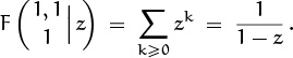
It’s our old friend, the geometric series; F(a₁, . . . , a_m; b₁, . . . , b_n; z) is called hypergeometric because it includes the geometric series F(1, 1; 1; z) as a very special case.

The general case m = 1 and n = 0 is, in fact, easy to sum in closed form,

using (5.13) and (5.14). If we replace a by –a and z by –z, we get the binomial theorem,

A negative integer as upper parameter causes the infinite series to become finite, since whenever k > a ≥ 0 and a is an integer.

The general case m = 0, n = 1 is another famous series, but it’s not as well known in the literature of discrete mathematics:

This function I_b–1 is called a “modified Bessel function” of order b – 1. The special case b = 1 gives us , which is the interesting series ∑_k≥0 z^k/k!².

The special case m = n = 1 is called a “confluent hypergeometric series” and often denoted by the letter M:

This function, which has important applications to engineering, was introduced by Ernst Kummer.

By now a few of us are wondering why we haven’t discussed convergence of the infinite series (5.76). The answer is that we can ignore convergence if we are using z simply as a formal symbol. It is not difficult to verify that formal infinite sums of the form ∑_k≥n α_kz^k with –∞ < n < ∞ form a field, if the coefficients α_k lie in a field. We can add, subtract, multiply, divide, differentiate, and do functional composition on such formal sums without worrying about convergence; any identities we derive will still be formally true. For example, the hypergeometric doesn’t converge for any nonzero z; yet we’ll see in Chapter 7 that we can still use it to solve problems. On the other hand, whenever we replace z by a particular numerical value, we do have to be sure that the infinite sum is well defined.

We didn’t discuss convergence of (5.56), (5.57), (5.58), . . . either.

The next step up in complication is actually the most famous hypergeometric of all. In fact, it was the hypergeometric series until about 1870, when everything was generalized to arbitrary m and n. This one has two upper parameters and one lower parameter:

It is often called the Gaussian hypergeometric, because many of its subtle properties were first proved by Gauss in his doctoral dissertation of 1812 [143], although Euler [118] and Pfaff [292] had already discovered some remarkable things about it. One of its important special cases is

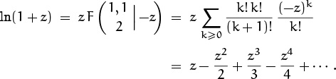
Notice that z^–1 ln(1 + z) is a hypergeometric function, but ln(1 + z) itself cannot be hypergeometric, since a hypergeometric series always has the value 1 when z = 0.

“There must be many universities to-day where 95 per cent, if not 100 per cent, of the functions studied by physics, engineering, and even mathematics students, are covered by this single symbol F(a, b; c; x).”

—W. W. Sawyer [318]

So far hypergeometrics haven’t actually done anything for us except provide an excuse for name-dropping. But we’ve seen that several very different functions can all be regarded as hypergeometric; this will be the main point of interest in what follows. We’ll see that a large class of sums can be written as hypergeometric series in a “canonical” way, hence we will have a good filing system for facts about binomial coefficients.

What series are hypergeometric? It’s easy to answer this question if we look at the ratio between consecutive terms:

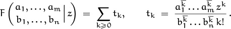
The first term is t₀ = 1, and the other terms have ratios given by

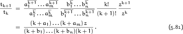
This is a rational function of k, that is, a quotient of polynomials in k. According to the Fundamental Theorem of Algebra, any rational function of k can be factored over the complex numbers and put into this form. The a’s are the negatives of the roots of the polynomial in the numerator, and the b’s are the negatives of the roots of the polynomial in the denominator. If the denominator doesn’t already contain the special factor (k + 1), we can include (k + 1) in both numerator and denominator. A constant factor remains, and we can call it z. Therefore hypergeometric series are precisely those series whose first term is 1 and whose term ratio t_k+1/t_k is a rational function of k.

Suppose, for example, that we’re given an infinite series with term ratio

a rational function of k. The numerator polynomial splits nicely into two factors, (k + 2)(k + 5), and the denominator is 4(k + i/2)(k – i/2). Since the denominator is missing the required factor (k + 1), we write the term ratio as

and we can read off the results: The given series is

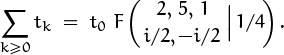
Thus, we have a general method for finding the hypergeometric representation of a given quantity S, when such a representation is possible: First we write S as an infinite series whose first term is nonzero. We choose a notation so that the series is ∑_k≥0 t_k with t₀ ≠ 0. Then we calculate t_k+1/t_k. If the term ratio is not a rational function of k, we’re out of luck. Otherwise we express it in the form (5.81); this gives parameters a₁, . . . , a_m, b₁, . . . , b_n, and an argument z, such that S = t₀ F(a₁, . . . , a_m; b₁, . . . , b_n; z).

(Now is a good time to do warmup exercise 11.)

Gauss’s hypergeometric series can be written in the recursively factored form

if we wish to emphasize the importance of term ratios.

Let’s try now to reformulate the binomial coefficient identities derived earlier in this chapter, expressing them as hypergeometrics. For example, let’s figure out what the parallel summation law,

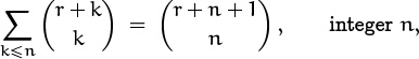
looks like in hypergeometric notation. We need to write the sum as an infinite series that starts at k = 0, so we replace k by n – k:

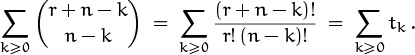
This series is formally infinite but actually finite, because the (n – k)! in the denominator will make t_k = 0 when k > n. (We’ll see later that 1/x! is defined for all x, and that 1/x! = 0 when x is a negative integer. But for now, let’s blithely disregard such technicalities until we gain more hypergeometric experience.) The term ratio is

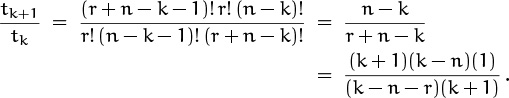
Furthermore t₀ = . Hence the parallel summation law is equivalent to the hypergeometric identity

Dividing through by gives a slightly simpler version,

Let’s do another one. The term ratio of identity (5.16),

is (k – m)/(r – m + k + 1) = (k + 1)(k – m)(1)/(k – m + r + 1)(k + 1), after we replace k by m – k; hence (5.16) gives a closed form for

This is essentially the same as the hypergeometric function on the left of (5.82), but with m in place of n and r + 1 in place of –r. Therefore identity (5.16) could have been derived from (5.82), the hypergeometric version of (5.9). (No wonder we found it easy to prove (5.16) by using (5.9).)

First derangements, now degenerates.

Before we go further, we should think about degenerate cases, because hypergeometrics are not defined when a lower parameter is zero or a negative integer. We usually apply the parallel summation identity when r and n are positive integers; but then –n–r is a negative integer and the hypergeometric (5.76) is undefined. How then can we consider (5.82) to be legitimate? The answer is that we can take the limit of as → 0.

We will look at such things more closely later in this chapter, but for now let’s just be aware that some denominators can be dynamite. It is interesting, however, that the very first sum we’ve tried to express hypergeometrically has turned out to be degenerate.

(We proved the identities originally for integer r, and used the polynomial argument to show that they hold in general. Now we’re proving them first for irrational r, and using a limiting argument to show that they hold for integers!)

Another possibly sore point in our derivation of (5.82) is that we expanded as (r + n – k)!/r! (n – k)!. This expansion fails when r is a negative integer, because (–m)! has to be ∞ if the law

0! = 0 · (–1) · (–2) · . . . · (–m + 1) · (–m)!

is going to hold. Again, we need to approach integer results by considering a limit of r + as → 0.

But we defined the factorial representation only when r is an integer! If we want to work effectively with hypergeometrics, we need a factorial function that is defined for all complex numbers. Fortunately there is such a function, and it can be defined in many ways. Here’s one of the most useful definitions of z!, actually a definition of 1/z!:

(See exercise 21. Euler [99, 100, 72] discovered this when he was 22 years old.) The limit can be shown to exist for all complex z, and it is zero only when z is a negative integer. Another significant definition is

This integral exists only when the real part of z exceeds –1, but we can use the formula

to extend the definition to all complex z (except negative integers). Still another definition comes from Stirling’s interpolation of ln z! in (5.47). All of these approaches lead to the same generalized factorial function.

There’s a very similar function called the Gamma function, which relates to ordinary factorials somewhat as rising powers relate to falling powers. Standard reference books often use factorials and Gamma functions simultaneously, and it’s convenient to convert between them if necessary using the following formulas:

We can use these generalized factorials to define generalized factorial powers, when z and w are arbitrary complex numbers:

How do you write z to the power, when is the complex conjugate of w?

The only proviso is that we must use appropriate limiting values when these formulas give ∞/∞. (The formulas never give 0/0, because factorials and Gamma-function values are never zero.) A binomial coefficient can be written

when z and w are any complex numbers whatever.

I see, the lower index arrives at its limit first. That’s why is zero when w is a negative integer. The value is infinite when z is a negative integer and w is not an integer.

Armed with generalized factorial tools, we can return to our goal of reducing the identities derived earlier to their hypergeometric essences. The binomial theorem (5.13) turns out to be neither more nor less than (5.77), as we might expect. So the next most interesting identity to try is Vandermonde’s convolution (5.27):

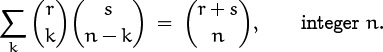
The kth term here is

and we are no longer too shy to use generalized factorials in these expressions. Whenever t_k contains a factor like (α + k)!, with a plus sign before the k, we get (α + k + 1)!/(α + k)! = k + α + 1 in the term ratio t_k+1/t_k, by (5.85); this contributes the parameter ‘α + 1’ to the corresponding hypergeometric—as an upper parameter if (α + k)! was in the numerator of t_k, but as a lower parameter otherwise. Similarly, a factor like (α – k)! leads to (α – k – 1)!/(α – k)! = (–1)/(k – α); this contributes ‘–α’ to the opposite set of parameters (reversing the roles of upper and lower), and negates the hypergeometric argument. Factors like r!, which are independent of k, go into t₀ but disappear from the term ratio. Using such tricks we can predict without further calculation that the term ratio of (5.27) is

times (–1)² = 1, and Vandermonde’s convolution becomes

We can use this equation to determine F(a, b; c; z) in general, when z = 1 and when b is a negative integer.

Let’s rewrite (5.91) in a form so that table lookup is easy when a new sum needs to be evaluated. The result turns out to be

Vandermonde’s convolution (5.27) covers only the case that one of the upper parameters, say b, is a nonpositive integer; but Gauss [143] proved that (5.92) is valid also when a, b, c are complex numbers whose real parts satisfy ℜc > ℜa + ℜb. In other cases, the infinite series doesn’t converge. When b = –n, the identity can be written more conveniently with factorial powers instead of Gamma functions:

A few weeks ago, we were studying what Gauss had done in kindergarten. Now we’re studying stuff beyond his Ph.D. thesis. Is this intimidating or what?

It turns out that all five of the identities in Table 169 are special cases of Vandermonde’s convolution; formula (5.93) covers them all, when proper attention is paid to degenerate situations.

Notice that (5.82) is just the special case a = 1 of (5.93). Therefore we don’t really need to remember (5.82); and we don’t really need the identity (5.9) that led us to (5.82), even though Table 174 said that it was memorable. A computer program for formula manipulation, faced with the problem of evaluating , could convert the sum to a hypergeometric and plug into the general identity for Vandermonde’s convolution.

Problem 1 in Section 5.2 asked for the value of

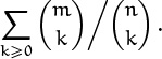
This problem is a natural for hypergeometrics, and after a bit of practice any hypergeometer can read off the parameters immediately as F(1, –m; –n; 1). Hmmm; that problem was yet another special takeoff on Vandermonde!

The sum in Problem 2 and Problem 4 likewise yields F(2, 1 – n; 2 – m; 1). (We need to replace k by k + 1 first.) And the “menacing” sum in Problem 6 turns out to be just F(n + 1, –n; 2; 1). Is there nothing more to sum, besides disguised versions of Vandermonde’s powerful convolution?

Well, yes, Problem 3 is a bit different. It deals with a special case of the general sum considered in (5.74), and this leads to a closed-form expression for

We also proved something new in (5.55), when we looked at the coefficients of (1 – z)^r(1 + z)^r:

This is called Kummer’s formula when it’s generalized to complex numbers:

Kummer was a summer.

(Ernst Kummer [229] proved this in 1836.)

The summer of ’36.

It’s interesting to compare these two formulas. Replacing c by 1–2n–a, we find that the results are consistent if and only if

when n is a positive integer. Suppose, for example, that n = 3; then we should have –6!/3! = lim_x→–3 x!/(2x)!. We know that (–3)! and (–6)! are both infinite; but we might choose to ignore that difficulty and to imagine that (–3)! = (–3)(–4)(–5)(–6)!, so that the two occurrences of (–6)! will cancel. Such temptations must, however, be resisted, because they lead to the wrong answer! The limit of x!/(2x)! as x → –3 is not (–3)(–4)(–5) but rather –6!/3! = (–4)(–5)(–6), according to (5.95).

The right way to evaluate the limit in (5.95) is to use equation (5.87), which relates negative-argument factorials to positive-argument Gamma functions. If we replace x by –n – and let → 0, two applications of (5.87) give

Now sin(x + y) = sin x cos y + cos x sin y; so this ratio of sines is

by the methods of Chapter 9. Therefore, by (5.86), we have

as desired.

Let’s complete our survey by restating the other identities we’ve seen so far in this chapter, clothing them in hypergeometric garb. The triple-binomial sum in (5.29) can be written

When this one is generalized to complex numbers, it is called Dixon’s formula:

One of the most general formulas we’ve encountered is the triple-binomial sum (5.28), which yields Saalschütz’s identity:

(Historical note: Saalschütz [315] independently discovered this formula almost 100 years after Pfaff [292] had first published it. Taking the limit as n → ∞ yields equation (5.92).)

This formula gives the value at z = 1 of the general hypergeometric series with three upper parameters and two lower parameters, provided that one of the upper parameters is a nonpositive integer and that b₁ + b₂ = a₁ + a₂ + a₃ + 1. (If the sum of the lower parameters exceeds the sum of the upper parameters by 2 instead of by 1, the formula of exercise 25 can be used to express F(a₁, a₂, a₃; b₁, b₂; 1) in terms of two hypergeometrics that satisfy Saalschütz’s identity.)

Our hard-won identity in Problem 8 of Section 5.2 reduces to

Sigh. This is just the special case c = 1 of Saalschütz’s identity (5.97), so we could have saved a lot of work by going to hypergeometrics directly!

What about Problem 7? That extra-menacing sum gives us the formula

which is the first case we’ve seen with three lower parameters. So it looks new. But it really isn’t; the left-hand side can be replaced by a multiple of

using exercise 26, and Saalschütz’s identity wins again.

Well, that’s another deflating experience, but it’s also another reason to appreciate the power of hypergeometric methods.

(Historical note: The great relevance of hypergeometric series to binomial coefficient identities was first pointed out by George Andrews in 1974 [9, section 5].)

The convolution identities in Table 202 do not have hypergeometric equivalents, because their term ratios are rational functions of k only when t is an integer. Equations (5.64) and (5.65) aren’t hypergeometric even when t = 1. But we can take note of what (5.62) tells us when t has small integer values:

The first of these formulas gives the result of Problem 7 again, when the quantities (r, s, n) are replaced respectively by (1, m – 2n – 1, n – m).

Finally, the “unexpected” sum (5.20) gives us an unexpected hypergeometric identity that turns out to be quite instructive. Let’s look at it in slow motion. First we convert to an infinite sum,

The term ratio from (2m – k)! 2^k/m! (m – k)! is 2(k – m)/(k – 2m), so we have a hypergeometric identity with z = 2:

But look at the lower parameter ‘–2m’. Negative integers are verboten, so this identity is undefined!

It’s high time to look at such limiting cases carefully, as promised earlier, because degenerate hypergeometrics can often be evaluated by approaching them from nearby nondegenerate points. We must be careful when we do this, because different results can be obtained if we take limits in different ways. For example, here are two limits that turn out to be quite different when one of the upper parameters is increased by :

Similarly, we have defined ; this is not the same as . The proper way to treat (5.98) as a limit is to realize that the upper parameter –m is being used to make all terms of the series zero for k > m; this means that we want to make the following more precise statement:

Each term of this limit is well defined, because the denominator factor does not become zero until k > 2m. Therefore this limit gives us exactly the sum (5.20) we began with.