7. Generating Functions

The most powerful way to deal with sequences of numbers, as far as anybody knows, is to manipulate infinite series that “generate” those sequences. We’ve learned a lot of sequences and we’ve seen a few generating functions; now we’re ready to explore generating functions in depth, and to see how remarkably useful they are.

7.1 Domino Theory and Change

Generating functions are important enough, and for many of us new enough, to justify a relaxed approach as we begin to look at them more closely. So let’s start this chapter with some fun and games as we try to develop our intuitions about generating functions. We will study two applications of the ideas, one involving dominoes and the other involving coins.

How many ways T_n are there to completely cover a 2 × n rectangle with 2 × 1 dominoes? We assume that the dominoes are identical (either because they’re face down, or because someone has rendered them indistinguishable, say by painting them all red); thus only their orientations—vertical or horizontal—matter, and we can imagine that we’re working with domino-shaped tiles. For example, there are three tilings of a 2 × 3 rectangle, namely , , and ; so T₃ = 3.

To find a closed form for general T_n we do our usual first thing, look at small cases. When n = 1 there’s obviously just one tiling, ; and when n = 2 there are two, and .

“Let me count the ways.”

—E. B. Browning

How about when n = 0; how many tilings of a 2 × 0 rectangle are there? It’s not immediately clear what this question means, but we’ve seen similar situations before: There is one permutation of zero objects (namely the empty permutation), so 0! = 1. There is one way to choose zero things from n things (namely to choose nothing), so . There is one way to partition the empty set into zero nonempty subsets, but there are no such ways to partition a nonempty set; so . By such reasoning we can conclude that there’s just one way to tile a 2 × 0 rectangle with dominoes, namely to use no dominoes; therefore T₀ = 1. (This spoils the simple pattern T_n = n that holds when n = 1, 2, and 3; but that pattern was probably doomed anyway, since T₀ wants to be 1 according to the logic of the situation.) A proper understanding of the null case turns out to be useful whenever we want to solve an enumeration problem.

Let’s look at one more small case, n = 4. There are two possibilities for tiling the left edge of the rectangle—we put either a vertical domino or two horizontal dominoes there. If we choose a vertical one, the partial solution is and the remaining 2 × 3 rectangle can be covered in T₃ ways. If we choose two horizontals, the partial solution can be completed in T₂ ways. Thus T₄ = T₃ + T₂ = 5. (The five tilings are , , , , and .)

We now know the first five values of T_n:

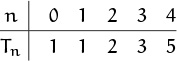
These look suspiciously like the Fibonacci numbers, and it’s not hard to see why: The reasoning we used to establish T₄ = T₃ + T₂ easily generalizes to T_n = T_n–1 + T_n–2, for n ≥ 2. Thus we have the same recurrence here as for the Fibonacci numbers, except that the initial values T₀ = 1 and T₁ = 1 are a little different. But these initial values are the consecutive Fibonacci numbers F₁ and F₂, so the T’s are just Fibonacci numbers shifted up one place:

T_n = F_n+1 ,    for n ≥ 0.

(We consider this to be a closed form for T_n, because the Fibonacci numbers are important enough to be considered “known.” Also, F_n itself has a closed form (6.123) in terms of algebraic operations.) Notice that this equation confirms the wisdom of setting T₀ = 1.

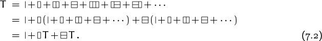
But what does all this have to do with generating functions? Well, we’re about to get to that—there’s another way to figure out what T_n is. This new way is based on a bold idea. Let’s consider the “sum” of all possible 2 × n tilings, for all n ≥ 0, and call it T:

To boldly go where no tiling has gone before.

(The first term ‘|’ on the right stands for the null tiling of a 2 × 0 rectangle.) This sum T represents lots of information. It’s useful because it lets us prove things about T as a whole rather than forcing us to prove them (by induction) about its individual terms.

The terms of this sum stand for tilings, which are combinatorial objects. We won’t be fussy about what’s considered legal when infinitely many tilings are added together; everything can be made rigorous, but our goal right now is to expand our consciousness beyond conventional algebraic formulas.

We’ve added the patterns together, and we can also multiply them—by juxtaposition. For example, we can multiply the tilings and to get the new tiling . But notice that multiplication is not commutative; that is, the order of multiplication counts: is different from .

Using this notion of multiplication it’s not hard to see that the null tiling plays a special role—it is the multiplicative identity. For instance, .

Now we can use domino arithmetic to manipulate the infinite sum T:

Every valid tiling occurs exactly once in each right side, so what we’ve done is reasonable even though we’re ignoring the cautions in Chapter 2 about “absolute convergence.” The bottom line of this equation tells us that everything in T is either the null tiling, or is a vertical tile followed by something else in T, or is two horizontal tiles followed by something else in T.

I have a gut feeling that these sums must converge, as long as the dominoes are small enough.

So now let’s try to solve the equation for T. Replacing the T on the left by |T and subtracting the last two terms on the right from both sides of the equation, we get

For a consistency check, here’s an expanded version:

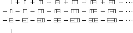
Every term in the top row, except the first, is cancelled by a term in either the second or third row, so our equation is correct.

So far it’s been fairly easy to make combinatorial sense of the equations we’ve been working with. Now, however, to get a compact expression for T we cross a combinatorial divide. With a leap of algebraic faith we divide both sides of equation (7.3) by to get

(Multiplication isn’t commutative, so we’re on the verge of cheating, by not distinguishing between left and right division. In our application it doesn’t matter, because | commutes with everything. But let’s not be picky, unless our wild ideas lead to paradoxes.)

The next step is to expand this fraction as a power series, using the rule

The null tiling |, which is the multiplicative identity for our combinatorial arithmetic, plays the part of 1, the usual multiplicative identity; and plays z. So we get the expansion

This is T, but the tilings are arranged in a different order than we had before. Every tiling appears exactly once in this sum; for example, appears in the expansion of .

We can get useful information from this infinite sum by compressing it down, ignoring details that are not of interest. For example, we can imagine that the patterns become unglued and that the individual dominoes commute with each other; then a term like becomes , because it contains four verticals and six horizontals. Collecting like terms gives us the series

T = | + + ² + ² + ³ + 2 ² + ⁴ + 3^{2 2} + ⁴ + · · ·.

The here represents the two terms of the old expansion, and , that have one vertical and two horizontal dominoes; similarly represents the three terms , , and . We’re essentially treating and as ordinary (commutative) variables.

We can find a closed form for the coefficients in the commutative version of T by using the binomial theorem:

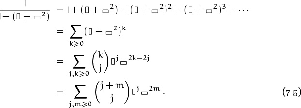
(The last step replaces k – j by m; this is legal because we have when 0 ≤ k < j.) We conclude that is the number of ways to tile a 2×(j+2m) rectangle with j vertical dominoes and 2m horizontal dominoes. For example, we recently looked at the 2 × 10 tiling , which involves four verticals and six horizontals; there are such tilings in all, so one of the terms in the commutative version of T is .

We can suppress even more detail by ignoring the orientation of the dominoes. Suppose we don’t care about the horizontal/vertical breakdown; we only want to know about the total number of 2 × n tilings. (This, in fact, is the number T_n we started out trying to discover.) We can collect the necessary information by simply substituting a single quantity, z, for and . And we might as well also replace | by 1, getting

Now I’m disoriented.

This is the generating function (6.117) for Fibonacci numbers, except for a missing factor of z in the numerator; so we conclude that the coefficient of zⁿ in T is F_n+1.

The compact representations , , and 1/(1–z–z²) that we have deduced for T are called generating functions, because they generate the coefficients of interest.

Incidentally, our derivation implies that the number of 2 × n domino tilings with exactly m pairs of horizontal dominoes is . (This follows because there are j = n – 2m vertical dominoes, hence there are

ways to do the tiling according to our formula.) We observed in Chapter 6 that is the number of Morse code sequences of length n that contain m dashes; in fact, it’s easy to see that 2×n domino tilings correspond directly to Morse code sequences. (The tiling corresponds to ‘’.) Thus domino tilings are closely related to the continuant polynomials we studied in Chapter 6. It’s a small world.

We have solved the T_n problem in two ways. The first way, guessing the answer and proving it by induction, was easier; the second way, using infinite sums of domino patterns and distilling out the coefficients of interest, was fancier. But did we use the second method only because it was amusing to play with dominoes as if they were algebraic variables? No; the real reason for introducing the second way was that the infinite-sum approach is a lot more powerful. The second method applies to many more problems, because it doesn’t require us to make magic guesses.

Let’s generalize up a notch, to a problem where guesswork will be beyond us. How many ways U_n are there to tile a 3 × n rectangle with dominoes?

The first few cases of this problem tell us a little: The null tiling gives U₀ = 1. There is no valid tiling when n = 1, since a 2 × 1 domino doesn’t fill a 3 × 1 rectangle, and since there isn’t room for two. The next case, n = 2, can easily be done by hand; there are three tilings, , , and , so U₂ = 3. (Come to think of it we already knew this, because the previous problem told us that T₃ = 3; the number of ways to tile a 3 × 2 rectangle is the same as the number to tile a 2 × 3.) When n = 3, as when n = 1, there are no tilings. We can convince ourselves of this either by making a quick exhaustive search or by looking at the problem from a higher level: The area of a 3 × 3 rectangle is odd, so we can’t possibly tile it with dominoes whose area is even. (The same argument obviously applies to any odd n.) Finally, when n = 4 there seem to be about a dozen tilings; it’s difficult to be sure about the exact number without spending a lot of time to guarantee that the list is complete.

So let’s try the infinite-sum approach that worked last time:

Every non-null tiling begins with either or or ; but unfortunately the first two of these three possibilities don’t simply factor out and leave us with U again. The sum of all terms in U that begin with can, however, be written as V, where

is the sum of all domino tilings of a mutilated 3 × n rectangle that has its lower left corner missing. Similarly, the terms of U that begin with can be written Λ, where

consists of all rectangular tilings lacking their upper left corner. The series Λ is a mirror image of V. These factorizations allow us to write

And we can factor V and Λ as well, because such tilings can begin in only two ways:

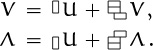
Now we have three equations in three unknowns (U, V, and Λ). We can solve them by first solving for V and Λ in terms of U, then plugging the results into the equation for U:

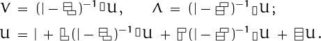
And the final equation can be solved for U, giving the compact formula

This expression defines the infinite sum U, just as (7.4) defines T.

The next step is to go commutative. Everything simplifies beautifully when we detach all the dominoes and use only powers of and :

I learned in another class about “regular expressions.” If I’m not mistaken, we can write

in the language of regular expressions; so there must be some connection between regular expressions and generating functions.

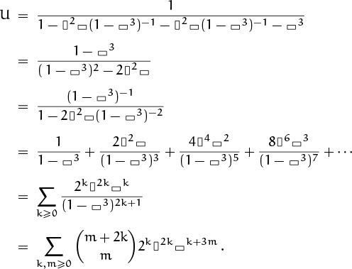
(This derivation deserves careful scrutiny. The last step uses the formula , identity (5.56).) Let’s take a good look at the bottom line to see what it tells us. First, it says that every 3 × n tiling uses an even number of vertical dominoes. Moreover, if there are 2k verticals, there must be at least k horizontals, and the total number of horizontals must be k + 3m for some m ≥ 0. Finally, the number of possible tilings with 2k verticals and k + 3m horizontals is exactly .

We now are able to analyze the 3×4 tilings that left us doubtful when we began looking at the 3 × n problem. When n = 4 the total area is 12, so we need six dominoes altogether. There are 2k verticals and k + 3m horizontals, for some k and m; hence 2k + k + 3m = 6. In other words, k + m = 2. If we use no verticals, then k = 0 and m = 2; the number of possibilities is . (This accounts for the tiling .) If we use two verticals, then k = 1 and m = 1; there are such tilings. And if we use four verticals, then k = 2 and m = 0; there are such tilings, making a total of U₄ = 11. In general if n is even, this reasoning shows that , hence and the total number of 3 × n tilings is

As before, we can also substitute z for both and , getting a generating function that doesn’t discriminate between dominoes of particular persuasions. The result is

If we expand this quotient into a power series, we get

U = 1 + U₂ z³ + U₄ z⁶ + U₆ z⁹ + U₈ z¹² + · · · ,

a generating function for the numbers U_n. (There’s a curious mismatch between subscripts and exponents in this formula, but it is easily explained. The coefficient of z⁹, for example, is U₆, which counts the tilings of a 3 × 6 rectangle. This is what we want, because every such tiling contains nine dominoes.)

We could proceed to analyze (7.10) and get a closed form for the coefficients, but it’s better to save that for later in the chapter after we’ve gotten more experience. So let’s divest ourselves of dominoes for the moment and proceed to the next advertised problem, “change.”

How many ways are there to pay 50 cents? We assume that the payment must be made with pennies , nickels , dimes , quarters , and half-dollars . George Pólya [298] popularized this problem by showing that it can be solved with generating functions in an instructive way.

Ah yes, I remember when we had half-dollars.

Let’s set up infinite sums that represent all possible ways to give change, just as we tackled the domino problems by working with infinite sums that represent all possible domino patterns. It’s simplest to start by working with fewer varieties of coins, so let’s suppose first that we have nothing but pennies. The sum of all ways to leave some number of pennies (but just pennies) in change can be written

The first term stands for the way to leave no pennies, the second term stands for one penny, then two pennies, three pennies, and so on. Now if we’re allowed to use both pennies and nickels, the sum of all possible ways is

since each payment has a certain number of nickels chosen from the first factor and a certain number of pennies chosen from P. (Notice that N is not the sum , because such a sum includes many types of payment more than once. For example, the term treats and as if they were different, but we want to list each set of coins only once without respect to order.)

Similarly, if dimes are permitted as well, we get the infinite sum

which includes terms like when it is expanded in full. Each of these terms is a different way to make change. Adding quarters and then half-dollars to the realm of possibilities gives

Coins of the realm.

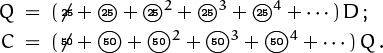
Our problem is to find the number of terms in C worth exactly 50¢.

A simple trick solves this problem nicely: We can replace by z, by z⁵, by z¹⁰, by z²⁵, and by z⁵⁰. Then each term is replaced by zⁿ, where n is the monetary value of the original term. For example, the term becomes z^50+10+5+5+1 = z⁷¹. The four ways of paying 13 cents, namely , , , and , each reduce to z¹³; hence the coefficient of z¹³ will be 4 after the z-substitutions are made.

Let P_n, N_n, D_n, Q_n, and C_n be the numbers of ways to pay n cents when we’re allowed to use coins that are worth at most 1, 5, 10, 25, and 50 cents, respectively. Our analysis tells us that these are the coefficients of zⁿ in the respective power series

 P = 1 + z + z² + z³ + z⁴ + · · · ,
N = (1 + z⁵ + z¹⁰ + z¹⁵ + z²⁰ + · · ·) P ,
D = (1 + z¹⁰ + z²⁰ + z³⁰ + z⁴⁰ + · · ·) N ,
Q = (1 + z²⁵ + z⁵⁰ + z⁷⁵ + z¹⁰⁰ + · · ·) D ,
C = (1 + z⁵⁰ + z¹⁰⁰ + z¹⁵⁰ + z²⁰⁰ + · · ·) Q .

How many pennies are there, really? If n is greater than, say, 10¹⁰, I bet that P_n = 0 in the “real world.”

Obviously P_n = 1 for all n ≥ 0. And a little thought proves that we have N_n = n/5 + 1: To make n cents out of pennies and nickels, we must choose either 0 or 1 or . . . or n/5 nickels, after which there’s only one way to supply the requisite number of pennies. Thus P_n and N_n are simple; but the values of D_n, Q_n, and C_n are increasingly more complicated.

One way to deal with these formulas is to realize that 1 + z^m + z^2m + · · · is just 1/(1 – z^m). Thus we can write

 P = 1/(1 – z) ,
N = P/(1 – z⁵) ,
D = N/(1 – z¹⁰) ,
Q = D/(1 – z²⁵) ,
C = Q/(1 – z⁵⁰) .

Multiplying by the denominators, we have

    (1 – z) P = 1 ,
  (1 – z⁵) N = P ,
(1 – z¹⁰) D = N ,
(1 – z²⁵) Q = D ,
(1 – z⁵⁰) C = Q .

Now we can equate coefficients of zⁿ in these equations, getting recurrence relations from which the desired coefficients can quickly be computed:

 P_n = P_n–1 + [n = 0] ,
N_n = N_n–5 + P_n ,
D_n = D_n–10 + N_n ,
Q_n = Q_n–25 + D_n ,
C_n = C_n–50 + Q_n .

For example, the coefficient of zⁿ in D = (1 – z²⁵)Q is equal to Q_n – Q_n–25; so we must have Q_n – Q_n–25 = D_n, as claimed.

We could unfold these recurrences and find, for example, that Q_n = D_n+D_n–25+D_n–50+D_n–75+ · · · , stopping when the subscripts get negative. But the non-iterated form is convenient because each coefficient is computed with just one addition, as in Pascal’s triangle.

Let’s use the recurrences to find C₅₀. First, C₅₀ = C₀ + Q₅₀; so we want to know Q₅₀. Then Q₅₀ = Q₂₅ + D₅₀, and Q₂₅ = Q₀ + D₂₅; so we also want to know D₅₀ and D₂₅. These D_n depend in turn on D₄₀, D₃₀, D₂₀, D₁₅, D₁₀, D₅, and on N₅₀, N₄₅, . . . , N₅. A simple calculation therefore suffices to determine all the necessary coefficients:

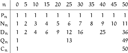
The final value in the table gives us our answer, C₅₀: There are exactly 50 ways to leave a 50-cent tip.

(Not counting the option of charging the tip to a credit card.)

How about a closed form for C_n? Multiplying the equations together gives us the compact expression

but it’s not obvious how to get from here to the coefficient of zⁿ. Fortunately there is a way; we’ll return to this problem later in the chapter.

More elegant formulas arise if we consider the problem of giving change when we live in a land that mints coins of every positive integer denomination ( ) instead of just the five we allowed before. The corresponding generating function is an infinite product of fractions,

and the coefficient of zⁿ when these factors are fully multiplied out is called p(n), the number of partitions of n. A partition of n is a representation of n as a sum of positive integers, disregarding order. For example, there are seven different partitions of 5, namely

5 = 4+1 = 3+2 = 3+1+1 = 2+2+1 = 2+1+1+1 = 1+1+1+1+1 ;

hence p(5) = 7. (Also p(2) = 2, p(3) = 3, p(4) = 5, and p(6) = 11; it begins to look as if p(n) is always a prime number. But p(7) = 15, spoiling the pattern.) There is no closed form for p(n), but the theory of partitions is a fascinating branch of mathematics in which many remarkable discoveries have been made. For example, Ramanujan proved that p(5n + 4) ≡ 0 (mod 5), p(7n + 5) ≡ 0 (mod 7), and p(11n + 6) ≡ 0 (mod 11), by making ingenious transformations of generating functions (see Andrews [11, Chapter 10]).

7.2 Basic Maneuvers

Now let’s look more closely at some of the techniques that make power series powerful.

First a few words about terminology and notation. Our generic generating function has the form

and we say that G(z), or G for short, is the generating function for the sequence g₀, g₁, g₂, . . ., which we also call g_n. The coefficient g_n of zⁿ in G(z) is often denoted [zⁿ] G(z), as in Section 5.4.

The sum in (7.12) runs over all n ≥ 0, but we often find it more convenient to extend the sum over all integers n. We can do this by simply regarding g_–1 = g_–2 = · · · = 0. In such cases we might still talk about the sequence g₀, g₁, g₂, . . ., as if the g_n’s didn’t exist for negative n.

Two kinds of “closed forms” come up when we work with generating functions. We might have a closed form for G(z), expressed in terms of z; or we might have a closed form for g_n, expressed in terms of n. For example, the generating function for Fibonacci numbers has the closed form z/(1 – z – z²); the Fibonacci numbers themselves have the closed form . The context will explain what kind of closed form is meant.

Now a few words about perspective. The generating function G(z) appears to be two different entities, depending on how we view it. Sometimes it is a function of a complex variable z, satisfying all the standard properties proved in calculus books. And sometimes it is simply a formal power series, with z acting as a placeholder. In the previous section, for example, we used the second interpretation; we saw several examples in which z was substituted for some feature of a combinatorial object in a “sum” of such objects. The coefficient of zⁿ was then the number of combinatorial objects having n occurrences of that feature.

If physicists can get away with viewing light sometimes as a wave and sometimes as a particle, mathematicians should be able to view generating functions in two different ways.

When we view G(z) as a function of a complex variable, its convergence becomes an issue. We said in Chapter 2 that the infinite series ∑_n≥0 g_nzⁿ converges (absolutely) if and only if there’s a bounding constant A such that the finite sums ∑_0≤n≤N |g_nzⁿ| never exceed A, for any N. Therefore it’s easy to see that if ∑_n≥0 g_nzⁿ converges for some value z = z₀, it also converges for all z with |z| < |z₀|. Furthermore, we must have ; hence, in the notation of Chapter 9, g_n = O(|1/z₀|ⁿ) if there is convergence at z₀. And conversely if g_n = O(Mⁿ), the series ∑_n≥0 g_nzⁿ converges for all |z| < 1/M. These are the basic facts about convergence of power series.

But for our purposes convergence is usually a red herring, unless we’re trying to study the asymptotic behavior of the coefficients. Nearly every operation we perform on generating functions can be justified rigorously as an operation on formal power series, and such operations are legal even when the series don’t converge. (The relevant theory can be found, for example, in Bell [23], Niven [282], and Henrici [182, Chapter 1].)

Furthermore, even if we throw all caution to the winds and derive formulas without any rigorous justification, we generally can take the results of our derivation and prove them by induction. For example, the generating function for the Fibonacci numbers converges only when |z| < 1/ϕ ≈ 0.618, but we didn’t need to know that when we proved the formula . The latter formula, once discovered, can be verified directly, if we don’t trust the theory of formal power series. Therefore we’ll ignore questions of convergence in this chapter; it’s more a hindrance than a help.

Even if we remove the tags from our mattresses.

So much for perspective. Next we look at our main tools for reshaping generating functions—adding, shifting, changing variables, differentiating, integrating, and multiplying. In what follows we assume that, unless stated otherwise, F(z) and G(z) are the generating functions for the sequences f_n and g_n. We also assume that the f_n’s and g_n’s are zero for negative n, since this saves us some bickering with the limits of summation.

It’s pretty obvious what happens when we add constant multiples of F and G together:

This gives us the generating function for the sequence αf_n + βg_n.

Shifting a generating function isn’t much harder. To shift G(z) right by m places, that is, to form the generating function for the sequence 0, . . . , 0, g₀, g₁, . . . = g_n–m with m leading 0’s, we simply multiply by z^m:

This is the operation we used (twice), along with addition, to deduce the equation (1 – z – z²)F(z) = z on our way to finding a closed form for the Fibonacci numbers in Chapter 6.

And to shift G(z) left m places—that is, to form the generating function for the sequence g_m, g_m+1, g_m+2, . . . = g_n+m with the first m elements discarded—we subtract off the first m terms and then divide by z^m:

(We can’t extend this last sum over all n unless g₀ = · · · = g_m–1 = 0.)

Replacing the z by a constant multiple is another of our tricks:

this yields the generating function for the sequence cⁿg_n. The special case c = –1 is particularly useful.

Often we want to bring down a factor of n into the coefficient. Differentiation is what lets us do that:

I fear d generating-function dz’s.

Shifting this right one place gives us a form that’s sometimes more useful,

This is the generating function for the sequence ng_n. Repeated differentiation would allow us to multiply g_n by any desired polynomial in n.

Integration, the inverse operation, lets us divide the terms by n:

(Notice that the constant term is zero.) If we want the generating function for g_n/n instead of g_n–1/n, we should first shift left one place, replacing G(t) by (G(t) – g₀)/t in the integral.

Finally, here’s how we multiply generating functions together:

As we observed in Chapter 5, this gives the generating function for the sequence h_n, the convolution of f_n and g_n. The sum h_n = ∑_k f_kg_n–k can also be written , because f_k = 0 when k < 0 and g_n–k = 0 when k > n. Multiplication/convolution is a little more complicated than the other operations, but it’s very useful—so useful that we will spend all of Section 7.5 below looking at examples of it.

Multiplication has several special cases that are worth considering as operations in themselves. We’ve already seen one of these: When F(z) = z^m we get the shifting operation (7.14). In that case the sum h_n becomes the single term g_n–m, because all f_k’s are 0 except for f_m = 1.

Another useful special case arises when F(z) is the familiar function 1/(1 – z) = 1 + z + z² + · · · ; then all f_k’s (for k ≥ 0) are 1 and we have the important formula

Multiplying a generating function by 1/(1–z) gives us the generating function for the cumulative sums of the original sequence.

Table 334 summarizes the operations we’ve discussed so far. To use all these manipulations effectively it helps to have a healthy repertoire of generating functions in stock. Table 335 lists the simplest ones; we can use those to get started and to solve quite a few problems.

Each of the generating functions in Table 335 is important enough to be memorized. Many of them are special cases of the others, and many of

Hint: If the sequence consists of binomial coefficients, its generating function usually involves a binomial, 1 ± z.

them can be derived quickly from the others by using the basic operations of Table 334; therefore the memory work isn’t very hard.

For example, let’s consider the sequence 1, 2, 3, 4, . . ., whose generating function 1/(1 – z)² is often useful. This generating function appears near the middle of Table 335, and it’s also the special case m = 1 of , which appears further down; it’s also the special case c = 2 of the closely related sequence . We can derive it from the generating function for 1, 1, 1, 1, . . . by taking cumulative sums as in (7.21); that is, by dividing 1/(1–z) by (1–z). Or we can derive it from 1, 1, 1, 1, . . . by differentiation, using (7.17).

OK, OK, I’m convinced already.

The sequence 1, 0, 1, 0, . . . is another one whose generating function can be obtained in many ways. We can obviously derive the formula ∑_n z²ⁿ = 1/(1 – z²) by substituting z² for z in the identity ∑_n zⁿ = 1/(1 – z); we can also apply cumulative summation to the sequence 1, –1, 1, –1, . . ., whose generating function is 1/(1 + z), getting 1/(1 + z)(1 – z) = 1/(1 – z²). And there’s also a third way, which is based on a general method for extracting the even-numbered terms g₀, 0, g₂, 0, g₄, 0, . . . of any given sequence: If we add G(–z) to G(+z) we get

therefore

The odd-numbered terms can be extracted in a similar way,

In the special case where g_n = 1 and G(z) = 1/(1–z), the generating function for 1, 0, 1, 0, . . . is .

Let’s try this extraction trick on the generating function for Fibonacci numbers. We know that ∑_n F_nzⁿ = z/(1 – z – z²); hence

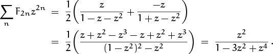
This generates the sequence F₀, 0, F₂, 0, F₄, . . . ; hence the sequence of alternate F’s, F₀, F₂, F₄, F₆, . . . = 0, 1, 3, 8, . . ., has a simple generating function:

7.3 Solving Recurrences

Now let’s focus our attention on one of the most important uses of generating functions: the solution of recurrence relations.

Given a sequence g_n that satisfies a given recurrence, we seek a closed form for g_n in terms of n. A solution to this problem via generating functions proceeds in four steps that are almost mechanical enough to be programmed on a computer:

1 Write down a single equation that expresses g_n in terms of other elements of the sequence. This equation should be valid for all integers n, assuming that g_–1 = g_–2 = · · · = 0.

2 Multiply both sides of the equation by zⁿ and sum over all n. This gives, on the left, the sum ∑_n g_nzⁿ, which is the generating function G(z). The right-hand side should be manipulated so that it becomes some other expression involving G(z).

3 Solve the resulting equation, getting a closed form for G(z).

4 Expand G(z) into a power series and read off the coefficient of zⁿ; this is a closed form for g_n.

This method works because the single function G(z) represents the entire sequence g_n in such a way that many manipulations are possible.

Example 1: Fibonacci numbers revisited.

For example, let’s rerun the derivation of Fibonacci numbers from Chapter 6. In that chapter we were feeling our way, learning a new method; now we can be more systematic. The given recurrence is

g₀ = 0 ;     g₁ = 1 ;
g_n = g_n–1 + g_{n – 2} ,     for n ≥ 2.

We will find a closed form for g_n by using the four steps above.

Step 1 tells us to write the recurrence as a “single equation” for g_n. We could say

but this is cheating. Step 1 really asks for a formula that doesn’t involve a case-by-case construction. The single equation

g_n = g_n–1 + g_n–2

works for n ≥ 2, and it also holds when n ≤ 0 (because we have g₀ = 0 and g_negative = 0). But when n = 1 we get 1 on the left and 0 on the right. Fortunately the problem is easy to fix, since we can add [n = 1] to the right; this adds 1 when n = 1, and it makes no change when n ≠ 1. So, we have

g_n = g_n–1 + g_n–2 + [n = 1];

this is the equation called for in Step 1.

Step 2 now asks us to transform the equation for g_n into an equation for G(z) = ∑_n g_nzⁿ. The task is not difficult:

Step 3 is also simple in this case; we have

which of course comes as no surprise.

Step 4 is the clincher. We carried it out in Chapter 6 by having a sudden flash of inspiration; let’s go more slowly now, so that we can get through Step 4 safely later, when we meet problems that are more difficult. What is

the coefficient of zⁿ when z/(1 – z – z²) is expanded in a power series? More generally, if we are given any rational function

where P and Q are polynomials, what is the coefficient [zⁿ] R(z)?

There’s one kind of rational function whose coefficients are particularly nice, namely

(The case ρ = 1 appears in Table 335; we get the general formula by substituting ρz for z and multiplying by a.) A finite sum of functions like (7.25),

also has nice coefficients,

We will show that every rational function R(z) such that R(0) ≠ ∞ can be expressed in the form

where S(z) has the form (7.26) and T(z) is a polynomial. Therefore there is a closed form for the coefficients [zⁿ] R(z). Finding S(z) and T(z) is equivalent to finding the “partial fraction expansion” of R(z).

Notice that S(z) = ∞ when z has the values 1/ρ₁, . . . , 1/ρ_l. Therefore the numbers ρ_k that we need to find, if we’re going to succeed in expressing R(z) in the desired form S(z) + T(z), must be the reciprocals of the numbers α_k where Q(α_k) = 0. (Recall that R(z) = P(z)/Q(z), where P and Q are polynomials; we have R(z) = ∞ only if Q(z) = 0.)

Suppose Q(z) has the form

Q(z) = q₀ + q₁z + · · · + q_mz^m ,    where q₀ ≠ 0 and q_m ≠ 0.

The “reflected” polynomial

Q^R(z) = q₀z^m + q₁z^m–1 + · · · + q_m

has an important relation to Q(z):

Q^R(z) = q₀(z – ρ₁) . . . (z – ρ_m)

       Q(z) = q₀(1 – ρ₁z) . . . (1 – ρ_mz) .

Thus, the roots of Q^R are the reciprocals of the roots of Q, and vice versa. We can therefore find the numbers ρ_k we seek by factoring the reflected polynomial Q^R(z).

For example, in the Fibonacci case we have

Q(z) = 1 – z – z² ;     Q^R(z) = z² – z – 1 .

The roots of Q^R can be found by setting (a, b, c) = (1, –1, –1) in the quadratic formula ; we find that they are

Therefore and .

Once we’ve found the ρ’s, we can proceed to find the partial fraction expansion. It’s simplest if all the roots are distinct, so let’s consider that special case first. We might as well state and prove the general result formally:

Rational Expansion Theorem for Distinct Roots.

If R(z) = P(z)/Q(z), where Q(z) = q₀(1 – ρ₁z) . . . (1 – ρ_lz) and the numbers (ρ₁, . . . , ρ_l) are distinct, and if P(z) is a polynomial of degree less than l, then

Proof: Let a₁, . . . , a_l be the stated constants. Formula (7.29) holds if R(z) = P(z)/Q(z) is equal to

And we can prove that R(z) = S(z) by showing that the function T(z) = R(z) – S(z) is not infinite as z → 1/ρ_k . For this will show that the rational function T(z) is never infinite; hence T(z) must be a polynomial. We also can show that T(z) → 0 as z → ∞; hence T(z) must be zero.

Impress your parents by leaving the book open at this page.

Let α_k = 1/ρ_k. To prove that lim_z→αk T(z) ≠ ∞, it suffices to show that lim_z→αk (z – α_k)T(z) = 0, because T(z) is a rational function of z. Thus we want to show that

The right-hand limit equals lim_z→αk a_k(z–α_k)/(1–ρ_kz) = –a_k/ρ_k, because (1 – ρ_kz) = –ρ_k(z – α_k) and (z – α_k)/(1 – ρ_jz) → 0 for j ≠ k. The left-hand limit is

by L’Hospital’s rule. Thus the theorem is proved.

Returning to the Fibonacci example, we have P(z) = z and ; hence Q′(z) = –1 – 2z, and

According to (7.29), the coefficient of ϕⁿ in [zⁿ] R(z) is therefore ; the coefficient of is . So the theorem tells us that , as in (6.123).

When Q(z) has repeated roots, the calculations become more difficult, but we can beef up the proof of the theorem and prove the following more general result:

General Expansion Theorem for Rational Generating Functions.

If R(z) = P(z)/Q(z), where Q(z) = q₀(1 – ρ₁z)^d₁ . . . (1 – ρ_lz)^d_l and the numbers (ρ₁, . . . , ρ_l) are distinct, and if P(z) is a polynomial of degree less than d₁ + · · · + d_l, then

where each f_k(n) is a polynomial of degree d_k – 1 with leading coefficient

This can be proved by induction on max(d₁, . . . , d_l), using the fact that

is a rational function whose denominator polynomial is not divisible by (1 – ρ_kz)^d_k for any k.

Example 2: A more-or-less random recurrence.

Now that we’ve seen some general methods, we’re ready to tackle new problems. Let’s try to find a closed form for the recurrence

It’s always a good idea to make a table of small cases first, and the recurrence lets us do that easily:

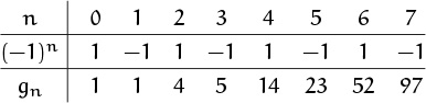
No closed form is evident, and this sequence isn’t even listed in Sloane’s Handbook [330]; so we need to go through the four-step process if we want to discover the solution.

Step 1 is easy, since we merely need to insert fudge factors to fix things when n < 2: The equation

g_n = g_n–1 + 2g_n–2 + (–1)ⁿ[n ≥ 0] + [n = 1]

holds for all integers n. Now we can carry out Step 2:

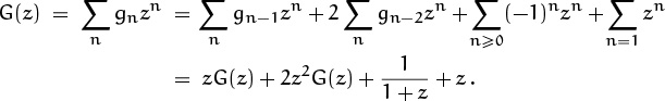
N.B.: The upper index on ∑_n=1 zⁿ is not missing!

(Incidentally, we could also have used instead of (–1)ⁿ[n ≥ 0], thereby getting by the binomial theorem.) Step 3 is elementary algebra, which yields

And that leaves us with Step 4.

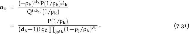
The squared factor in the denominator is a bit troublesome, since we know that repeated roots are more complicated than distinct roots; but there it is. We have two roots, ρ₁ = 2 and ρ₂ = –1; the general expansion theorem (7.30) tells us that

g_n = a₁2ⁿ + (a₂n + c)(–1)ⁿ

for some constant c, where

(The second formula for a_k in (7.31) is easier to use than the first one when the denominator has nice factors. We simply substitute z = 1/ρ_k everywhere in R(z), except in the factor where this gives zero, and divide by (d_k – 1)!; this gives the coefficient of .) Plugging in n = 0 tells us that the value of the remaining constant c had better be ; hence our answer is

It doesn’t hurt to check the cases n = 1 and 2, just to be sure that we didn’t foul up. Maybe we should even try n = 3, since this formula looks weird. But it’s correct, all right.

Could we have discovered (7.33) by guesswork? Perhaps after tabulating a few more values we may have observed that g_n+1 ≈ 2g_n when n is large. And with chutzpah and luck we might even have been able to smoke out the constant . But it sure is simpler and more reliable to have generating functions as a tool.

Example 3: Mutually recursive sequences.

Sometimes we have two or more recurrences that depend on each other. Then we can form generating functions for both of them, and solve both by a simple extension of our four-step method.

For example, let’s return to the problem of 3 × n domino tilings that we explored earlier this chapter. If we want to know only the total number of ways, U_n, to cover a 3 × n rectangle with dominoes, without breaking this number down into vertical dominoes versus horizontal dominoes, we needn’t go into as much detail as we did before. We can merely set up the recurrences

Here V_n is the number of ways to cover a 3 × n rectangle-minus-corner, using (3n – 1)/2 dominoes. These recurrences are easy to discover, if we consider the possible domino configurations at the rectangle’s left edge, as before. Here are the values of U_n and V_n for small n:

Let’s find closed forms, in four steps. First (Step 1), we have

U_n = 2V_n–1 + U_n–2 + [n = 0] ,     V_n = U_n–1 + V_n–2 ,

for all n. Hence (Step 2),

U(z) = 2zV(z) + z²U(z) + 1 ,     V(z) = zU(z) + z²V(z) .

Now (Step 3) we must solve two equations in two unknowns; but these are easy, since the second equation yields V(z) = zU(z)/(1 – z²); we find

(We had this formula for U(z) in (7.10), but with z³ instead of z². In that derivation, n was the number of dominoes; now it’s the width of the rectangle.)

The denominator 1 – 4z² + z⁴ is a function of z²; this is what makes U_2n+1 = 0 and V_2n = 0, as they should be. We can take advantage of this nice property of z² by retaining z² when we factor the denominator: We need not take 1 – 4z² + z⁴ all the way to a product of four factors (1 – ρ_kz), since two factors of the form (1 – ρ_kz²) will be enough to tell us the coefficients. In other words if we consider the generating function

we will have V(z) = zW(z²) and U(z) = (1 – z²)W(z²); hence V_2n+1 = W_n and U_2n = W_n – W_n–1. We save time and energy by working with the simpler function W(z).

The factors of 1 – 4z + z² are and , and they can also be written and because this polynomial is its own reflection. Thus it turns out that we have

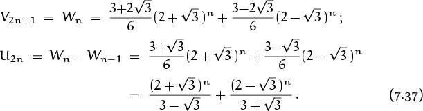
This is the desired closed form for the number of 3 × n domino tilings.

Incidentally, we can simplify the formula for U_2n by realizing that the second term always lies between 0 and 1. The number U_2n is an integer, so we have

In fact, the other term is extremely small when n is large, because . This needs to be taken into account if we try to use formula (7.38) in numerical calculations. For example, a fairly expensive name-brand hand calculator comes up with 413403.0005 when asked to compute . This is correct to nine significant figures; but the true value is slightly less than 413403, not slightly greater. Therefore it would be a mistake to take the ceiling of 413403.0005; the correct answer, U₂₀ = 413403, is obtained by rounding to the nearest integer. Ceilings can be hazardous.

I’ve known slippery floors too.

Example 4: A closed form for change.

When we left the problem of making change, we had just calculated the number of ways to pay 50¢. Let’s try now to count the number of ways there are to change a dollar, or a million dollars—still using only pennies, nickels, dimes, quarters, and halves.

The generating function derived earlier is

this is a rational function of z with a denominator of degree 91. Therefore we can decompose the denominator into 91 factors and come up with a 91-term “closed form” for C_n, the number of ways to give n cents in change. But that’s too horrible to contemplate. Can’t we do better than the general method suggests, in this particular case?

One ray of hope suggests itself immediately, when we notice that the denominator is almost a function of z⁵. The trick we just used to simplify the calculations by noting that 1 – 4z² + z⁴ is a function of z² can be applied to C(z), if we replace 1/(1 – z) by (1 + z + z² + z³ + z⁴)/(1 – z⁵):

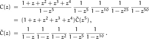
The compressed function Č(z) has a denominator whose degree is only 19, so it’s much more tractable than the original. This new expression for C(z) shows us, incidentally, that C_5n = C_5n+1 = C_5n+2 = C_5n+3 = C_5n+4; and indeed, this set of equations is obvious in retrospect: The number of ways to leave a 53¢ tip is the same as the number of ways to leave a 50¢ tip, because the number of pennies is predetermined modulo 5.

But Č(z) still doesn’t have a really simple closed form based on the roots of the denominator. The easiest way to compute the coefficients of Č(z) is probably to recognize that each of the denominator factors is a divisor of 1 – z¹⁰. Hence we can write

Now we’re also getting compressed reasoning.

The actual value of A(z), for the curious, is

(1 + z + ··· + z⁹)²(1 + z² + ··· + z⁸)(1 + z⁵)
   = 1 + 2z + 4z² + 6z³ + 9z⁴ + 13z⁵ + 18z⁶ + 24z⁷
     + 31z⁸ + 39z⁹ + 45z¹⁰ + 52z¹¹ + 57z¹² + 63z¹³ + 67z¹⁴ + 69z¹⁵
     + 69z¹⁶ + 67z¹⁷ + 63z¹⁸ + 57z¹⁹ + 52z²⁰ + 45z²¹ + 39z²² + 31z²³
     + 24z²⁴ + 18z²⁵ + 13z²⁶ + 9z²⁷ + 6z²⁸ + 4z²⁹ + 2z³⁰ + z³¹ .

Finally, since , we can determine the coefficient Č_n = [zⁿ] Č(z) as follows, when n = 10q + r and 0 ≤ r < 10:

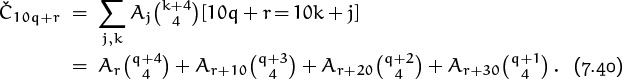
This gives ten cases, one for each value of r; but it’s a pretty good closed form, compared with alternatives that involve powers of complex numbers.

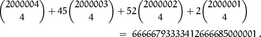
For example, we can use this expression to deduce the value of C_50q = Č_10q. Then r = 0 and we have

The number of ways to change 50¢ is ; the number of ways to change $1 is ; and the number of ways to change $1,000,000 is

Example 5: A divergent series.

Now let’s try to get a closed form for the numbers g_n defined by

g₀ = 1 ;
g_n = ng_n–1 ,     for n > 0.

Nowadays people are talking femto seconds.

After staring at this for a few nanoseconds we realize that g_n is just n!; in fact, the method of summation factors described in Chapter 2 suggests this answer immediately. But let’s try to solve the recurrence with generating functions, just to see what happens. (A powerful technique should be able to handle easy recurrences like this, as well as others that have answers we can’t guess so easily.)

The equation

g_n = ng_n–1 + [n = 0]

holds for all n, and it leads to

To complete Step 2, we want to express ∑_n ng_n–1 zⁿ in terms of G(z), and the basic maneuvers in Table 334 suggest that the derivative G′(z) = ∑_n ng_nz^n–1 is somehow involved. So we steer toward that kind of sum:

Let’s check this equation, using the values of g_n for small n. Since

 G = 1 + z + 2z² + 6z³ + 24z⁴ + · · · ,
G′ =   1 + 4z + 18z² + 96z³ + · · · ,

we have

z²G′ =       z² + 4z³ + 18z⁴ + 96z⁵ + · · · ,
  zG =   z + z² + 2z³ + 6z⁴ + 24z⁵ + · · · ,
   1 = 1 .

These three lines add up to G, so we’re fine so far. Incidentally, we often find it convenient to write ‘G’ instead of ‘G(z)’; the extra ‘(z)’ just clutters up the formula when we aren’t changing z.

Step 3 is next, and it’s different from what we’ve done before because we have a differential equation to solve. But this is a differential equation that we can handle with the hypergeometric series techniques of Section 5.6; those techniques aren’t too bad. (Readers who are unfamiliar with hypergeometrics needn’t worry—this will be quick.)

“This will be quick.” That’s what the doctor said just before he stuck me with that needle. Come to think of it, “hypergeometric” sounds a lot like “hypodermic.”

First we must get rid of the constant ‘1’, so we take the derivative of both sides:

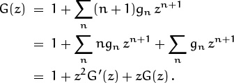
G′ = (z²G′ + zG + 1)′ = (2zG′ + z²G″) + (G + zG′)
                  = z²G″ + 3zG′ + G .

The theory in Chapter 5 tells us to rewrite this using the ϑ operator, and we know from exercise 6.13 that

ϑG = zG′ ,     ϑ²G = z²G″ + zG′ .

Therefore the desired form of the differential equation is

ϑG = zϑ²G + 2zϑG + zG = z(ϑ + 1)²G .

According to (5.109), the solution with g₀ = 1 is the hypergeometric series F(1, 1; ; z).

Step 3 was more than we bargained for; but now that we know what the function G is, Step 4 is easy—the hypergeometric definition (5.76) gives us the power series expansion:

We’ve confirmed the closed form we knew all along, g_n = n!.

Notice that the technique gave the right answer even though G(z) diverges for all nonzero z. The sequence n! grows so fast, the terms |n! zⁿ| approach ∞ as n → ∞, unless z = 0. This shows that formal power series can be manipulated algebraically without worrying about convergence.

Example 6: A recurrence that goes all the way back.

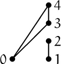
Let’s close this section by applying generating functions to a problem in graph theory. A fan of order n is a graph on the vertices {0, 1, . . . , n} with 2n – 1 edges defined as follows: Vertex 0 is connected by an edge to each of the other n vertices, and vertex k is connected by an edge to vertex k + 1, for 1 ≤ k < n. Here, for example, is the fan of order 4, which has five vertices and seven edges.

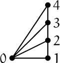
The problem of interest: How many spanning trees f_n are in such a graph? A spanning tree is a subgraph containing all the vertices, and containing enough edges to make the subgraph connected yet not so many that it has a cycle. It turns out that every spanning tree of a graph on n + 1 vertices has exactly n edges. With fewer than n edges the subgraph wouldn’t be connected, and with more than n it would have a cycle; graph theory books prove this.

There are ways to choose n edges from among the 2n – 1 present in a fan of order n, but these choices don’t always yield a spanning tree. For instance the subgraph

has four edges but is not a spanning tree; it has a cycle from 0 to 4 to 3 to 0, and it has no connection between {1, 2} and the other vertices. We want to count how many of the choices actually do yield spanning trees.

Let’s look at some small cases. It’s pretty easy to enumerate the spanning trees for n = 1, 2, and 3:

(We need not show the labels on the vertices, if we always draw vertex 0 at the left.) What about the case n = 0? At first it seems reasonable to set f₀ = 1; but we’ll take f₀ = 0, because the existence of a fan of order 0 (which should have 2n – 1 = –1 edges) is dubious.

Our four-step procedure tells us to find a recurrence for f_n that holds for all n. We can get a recurrence by observing how the topmost vertex (vertex n) is connected to the rest of the spanning tree. If it’s not connected to vertex 0, it must be connected to vertex n – 1, since it must be connected to the rest of the graph. In this case, any of the f_n–1 spanning trees for the remaining fan (on the vertices 0 through n – 1) will complete a spanning tree for the whole graph. Otherwise vertex n is connected to 0, and there’s some number k ≤ n such that vertices n, n – 1, . . . , k are connected directly but the edge between k and k – 1 is not present. Then there can’t be any edges between 0 and {n – 1, . . . , k}, or there would be a cycle. If k = 1, the spanning tree is therefore determined completely. And if k > 1, any of the f_k–1 ways to produce a spanning tree on {0, 1, . . . , k–1} will yield a spanning tree on the whole graph. For example, here’s what this analysis produces when n = 4:

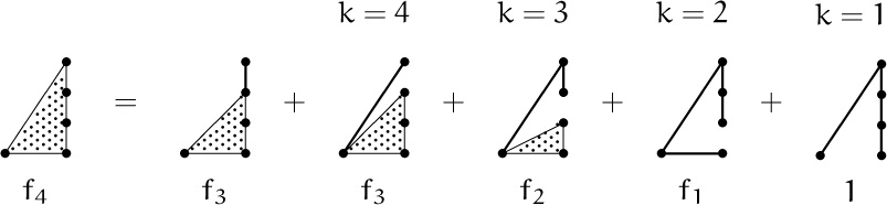
The general equation, valid for n ≥ 1, is

f_n = f_n–1 + f_n–1 + f_n–2 + f_n–3 + · · · + f₁ + 1 .

(It almost seems as though the ‘1’ on the end is f₀ and we should have chosen f₀ = 1; but we will doggedly stick with our choice.) A few changes suffice to make the equation valid for all integers n:

This is a recurrence that “goes all the way back” from f_n–1 through all previous values, so it’s different from the other recurrences we’ve seen so far in this chapter. We used a special method to get rid of a similar right-side sum in Chapter 2, when we solved the quicksort recurrence (2.12); namely, we subtracted one instance of the recurrence from another (f_n+1 – f_n). This trick would get rid of the ∑ now, as it did then; but we’ll see that generating functions allow us to work directly with such sums. (And it’s a good thing that they do, because we will be seeing much more complicated recurrences before long.)

Step 1 is finished; Step 2 is where we need to do a new thing:

The key trick here was to change zⁿ to z^k z^n–k; this made it possible to express the value of the double sum in terms of F(z), as required in Step 2.

Now Step 3 is simple algebra, and we find

Those of us with a zest for memorization will recognize this as the generating function (7.24) for the even-numbered Fibonacci numbers. So, we needn’t go through Step 4; we have found a somewhat surprising answer to the spans-of-fans problem:

7.4 Special Generating Functions

Step 4 of the four-step procedure becomes much easier if we know the coefficients of lots of different power series. The expansions in Table 335 are quite useful, as far as they go, but many other types of closed forms are possible. Therefore we ought to supplement that table with another one, which lists power series that correspond to the “special numbers” considered in Chapter 6.

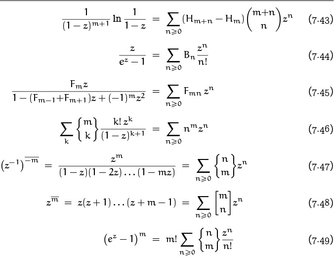
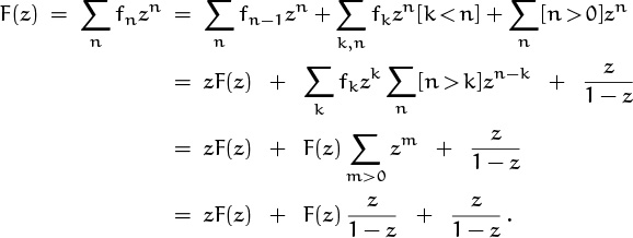
Table 351 is the database we need. The identities in this table are not difficult to prove, so we needn’t dwell on them; this table is primarily for reference when we meet a new problem. But there’s a nice proof of the first formula, (7.43), that deserves mention: We start with the identity

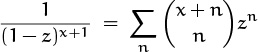
and differentiate it with respect to x. On the left, (1 – z)^–x–1 is equal to e^{(x+1) ln(1/(1–z))}, so d/dx contributes a factor of ln (1/(1 – z)). On the right, the numerator of is (x + n) . . . (x + 1), and d/dx splits this into n terms whose sum is equivalent to multiplying by

Replacing x by m gives (7.43). Notice that H_x+n – H_x is meaningful even when x is not an integer.

By the way, this method of differentiating a complicated product—leaving it as a product—is usually better than expressing the derivative as a sum. For example the right side of

would be a lot messier written out as a sum.

The general identities in Table 351 include many important special cases. For example, (7.43) simplifies to the generating function for H_n when m = 0:

This equation can also be derived in other ways; for example, we can take the power series for ln (1/(1 – z)) and divide it by 1 – z to get cumulative sums.

Identities (7.51) and (7.52) involve the respective ratios and , which have the undefined form 0/0 when n ≥ m. However, there is a way to give them a proper meaning using the Stirling polynomials of (6.45), because we have

Thus, for example, the case m = 1 of (7.51) should not be regarded as the power series , but rather as

Identities (7.53), (7.54), (7.55), and (7.56) are “double generating functions” or “super generating functions” because they have the form G(w, z) = ∑_m,n g_m,nw^mzⁿ. The coefficient of w^m is a generating function in the variable z; the coefficient of zⁿ is a generating function in the variable w. Equation (7.56) can be put into the more symmetrical form

7.5 Convolutions

I always thought convolution was what happens to my brain when I try to do a proof.

The convolution of two given sequences f₀, f₁, . . . = f_n and g₀, g₁, . . . = g_n is the sequence f₀g₀, f₀g₁ + f₁g₀, . . . = ∑_k f_kg_n–k. We have observed in Sections 5.4 and 7.2 that convolution of sequences corresponds to multiplication of their generating functions. This fact makes it easy to evaluate many sums that would otherwise be difficult to handle.

Example 1: A Fibonacci convolution.

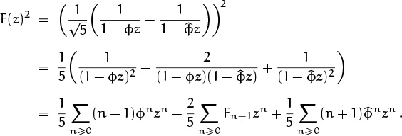
For example, let’s try to evaluate in closed form. This is the convolution of F_n with itself, so the sum must be the coefficient of zⁿ in F(z)², where F(z) is the generating function for F_n. All we have to do is figure out the value of this coefficient.

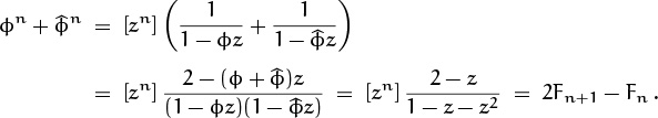
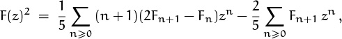
The generating function F(z) is z/(1–z–z²), a quotient of polynomials; so the general expansion theorem for rational functions tells us that the answer can be obtained from a partial fraction representation. We can use the general expansion theorem (7.30) and grind away; or we can use the fact that

Instead of expressing the answer in terms of ϕ and , let’s try for a closed form in terms of Fibonacci numbers. Recalling that , we have

Hence

and we have the answer we seek:

For example, when n = 3 this formula gives F₀F₃ + F₁F₂ + F₂F₁ + F₃F₀ = 0 + 1 + 1 + 0 = 2 on the left and (6F₄ – 4F₃)/5 = (18 – 8)/5 = 2 on the right.

Example 2: Harmonic convolutions.

The efficiency of a certain computer method called “samplesort” depends on the value of the sum

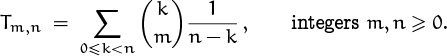
Exercise 5.58 obtains the value of this sum by a somewhat intricate double induction, using summation factors. It’s much easier to realize that T_m,n is just the nth term in the convolution of with . Both sequences have simple generating functions in Table 335:

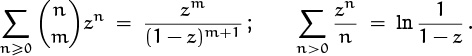
Therefore, by (7.43),

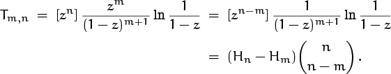
In fact, there are many more sums that boil down to this same sort of convolution, because we have

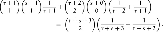
for all r and s. Equating coefficients of zⁿ gives the general identity

Because it’s so harmonic.

This seems almost too good to be true. But it checks, at least when n = 2:

Special cases like s = 0 are as remarkable as the general case.

And there’s more. We can use the convolution identity

to transpose H_r to the other side, since H_r is independent of k:

There’s still more: If r and s are nonnegative integers l and m, we can replace by and by ; then we can change k to k – l and n to n – m – l, getting

Even the special case l = m = 0 of this identity was difficult for us to handle in Chapter 2! (See (2.36).) We’ve come a long way.

Example 3: Convolutions of convolutions.

If we form the convolution of f_n and g_n, then convolve this with a third sequence h_n, we get a sequence whose nth term is

The generating function of this three-fold convolution is, of course, the threefold product F(z)G(z)H(z). In a similar way, the m-fold convolution of a sequence g_n with itself has nth term equal to

and its generating function is G(z)^m.

We can apply these observations to the spans-of-fans problem considered earlier (Example 6 in Section 7.3). It turns out that there’s another way to compute f_n, the number of spanning trees of an n-fan, based on the configurations of tree edges between the vertices {1, 2, . . . , n}: The edge between vertex k and vertex k + 1 may or may not be selected for the tree; and each of the ways to select these edges connects up certain blocks of adjacent vertices. For example, when n = 10 we might connect vertices {1, 2}, {3}, {4, 5, 6, 7}, and {8, 9, 10}:

Concrete blocks.

How many spanning trees can we make, by adding additional edges to vertex 0? We need to connect 0 to each of the four blocks; and there are two ways to join 0 with {1, 2}, one way to join it with {3}, four ways with {4, 5, 6, 7}, and three ways with {8, 9, 10}, or 2 · 1 · 4 · 3 = 24 ways altogether. Summing over all possible ways to make blocks gives us the following expression for the total number of spanning trees:

For example, f₄ = 4 + 3·1 + 2·2 + 1·3 + 2·1·1 + 1·2·1 + 1·1·2 + 1·1·1·1 = 21.

This is the sum of m-fold convolutions of the sequence 0, 1, 2, 3, . . ., for m = 1, 2, 3, . . . ; hence the generating function for f_n is

where G(z) is the generating function for 0, 1, 2, 3, . . ., namely z/(1 – z)². Consequently we have

as before. This approach to f_n is more symmetrical and appealing than the complicated recurrence we had earlier.

Example 4: A convoluted recurrence.

Our next example is especially important. In fact, it’s the “classic example” of why generating functions are useful in the solution of recurrences.

Suppose we have n + 1 variables x₀, x₁, . . . , x_n whose product is to be computed by doing n multiplications. How many ways C_n are there to insert parentheses into the product x₀· x₁·. . .· x_n so that the order of multiplication is completely specified? For example, when n = 2 there are two ways, x₀· (x₁· x₂) and (x₀ · x₁) · x₂. And when n = 3 there are five ways,

x₀ · (x₁ · (x₂ · x₃)) , x₀ · ((x₁ · x₂) · x₃) , (x₀ · x₁) · (x₂ · x₃) , (x₀ · (x₁ · x₂)) · x₃ , ((x₀ · x₁) · x₂) · x₃ .

Thus C₂ = 2 , C₃ = 5; we also have C₁ = 1 and C₀ = 1.

Let’s use the four-step procedure of Section 7.3. What is a recurrence for the C’s? The key observation is that there’s exactly one ‘ · ’ operation outside all of the parentheses, when n > 0; this is the final multiplication that ties everything together. If this ‘ · ’ occurs between x_k and x_k+1, there are C_k ways to fully parenthesize x₀ · . . . · x_k, and there are C_n–k–1 ways to fully parenthesize x_k+1 ·. . .· x_n; hence

C_n = C₀C_n–1 + C₁C_n–2 + · · · + C_n–1C₀ ,     if n > 0.

By now we recognize this expression as a convolution, and we know how to patch the formula so that it holds for all integers n:

Step 1 is now complete. Step 2 tells us to multiply by zⁿ and sum:

Lo and behold, the convolution has become a product, in the generating-function world. Life is full of surprises.

The authors jest.

Step 3 is also easy. We solve for C(z) by the quadratic formula:

But should we choose the + sign or the – sign? Both choices yield a function that satisfies C(z) = zC(z)² + 1, but only one of the choices is suitable for our problem. We might choose the + sign on the grounds that positive thinking is best; but we soon discover that this choice gives C(0) = ∞, contrary to the facts. (The correct function C(z) is supposed to have C(0) = C₀ = 1.) Therefore we conclude that

Finally, Step 4. What is [zⁿ] C(z)? The binomial theorem tells us that

hence, using (5.37),

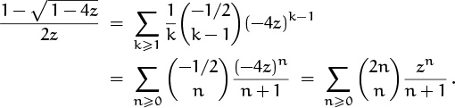
The number of ways to parenthesize, C_n, is .

We anticipated this result in Chapter 5, when we introduced the sequence of Catalan numbers 1, 1, 2, 5, 14, . . . = C_n. This sequence arises in dozens of problems that seem at first to be unrelated to each other [46], because many situations have a recursive structure that corresponds to the convolution recurrence (7.66).

So the convoluted recurrence has led us to an oft-recurring convolution.

For example, let’s consider the following problem: How many sequences a₁, a₂, . . . , a_2n of +1’s and –1’s have the property that

a₁ + a₂ + · · · + a_2n = 0

and have all their partial sums

a₁,  a₁ + a₂, . . . , a₁ + a₂ + · · · + a_2n

nonnegative? There must be n occurrences of +1 and n occurrences of –1. We can represent this problem graphically by plotting the sequence of partial sums as a function of n: The five solutions for n = 3 are

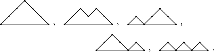
These are “mountain ranges” of width 2n that can be drawn with line segments of the forms and . It turns out that there are exactly C_n ways to do this, and the sequences can be related to the parenthesis problem in the following way: Put an extra pair of parentheses around the entire formula, so that there are n pairs of parentheses corresponding to the n multiplications. Now replace each ‘ · ’ by +1 and each ‘)’ by –1 and erase everything else. For example, the formula x₀ · ((x₁ · x₂) · (x₃ · x₄)) corresponds to the sequence +1, +1, –1, +1, +1, –1, –1, –1 by this rule. The five ways to parenthesize x₀ · x₁ · x₂ · x₃ correspond to the five mountain ranges for n = 3 shown above.

Moreover, a slight reformulation of our sequence-counting problem leads to a surprisingly simple combinatorial solution that avoids the use of generating functions: How many sequences a₀, a₁, a₂, . . . , a_2n of +1’s and –1’s have the property that

a₀ + a₁ + a₂ + · · · + a_2n = 1 ,

when all the partial sums

a₀,  a₀ + a₁,   a₀ + a₁ + a₂,   . . . ,   a₀ + a₁ + · · · + a_2n

are required to be positive? Clearly these are just the sequences of the previous problem, with the additional element a₀ = +1 placed in front. But the sequences in the new problem can be enumerated by a simple counting argument, using a remarkable fact discovered by George Raney [302] in 1959: If x₁, x₂, . . . , x_m is any sequence of integers whose sum is +1, exactly one of the cyclic shifts

x₁, x₂, . . . , x_m, x₂, . . . , x_m, x₁, . . . , x_m, x₁, . . . , x_m–1

has all of its partial sums positive. For example, consider the sequence 3, –5, 2, –2, 3, 0. Its cyclic shifts are

3, –5, 2, –2, 3, 0	–2, 3, 0, 3, –5, 2
–5, 2, –2, 3, 0, 3	3, 0, 3, –5, 2, –2 √
2, –2, 3, 0, 3, –5	0, 3, –5, 2, –2, 3

and only the one that’s checked has entirely positive partial sums.

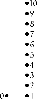
Raney’s lemma can be proved by a simple geometric argument. Let’s extend the sequence periodically to get an infinite sequence

x₁, x₂, . . . , x_m, x₁, x₂, . . . , x_m, x₁, x₂, . . . ;

thus we let x_m+k = x_k for all k > 0. If we now plot the partial sums s_n = x₁ + · · · + x_n as a function of n, the graph of s_n has an “average slope” of 1/m, because s_m+n = s_n + 1. For example, the graph corresponding to our example sequence 3, –5, 2, –2, 3, 0, 3, –5, 2, . . . begins as follows:

The entire graph can be contained between two lines of slope 1/m, as shown; we have m = 6 in the illustration. In general these bounding lines touch the graph just once in each cycle of m points, since lines of slope 1/m hit points with integer coordinates only once per m units. The unique lower point of intersection is the only place in the cycle from which all partial sums will be positive, because every other point on the curve has an intersection point within m units to its right.

Ah, if stock prices would only continue to rise like this.

With Raney’s lemma we can easily enumerate the sequences a₀, . . . , a_2n of +1’s and –1’s whose partial sums are entirely positive and whose total sum is +1. There are sequences with n occurrences of –1 and n + 1 occurrences of +1, and Raney’s lemma tells us that exactly 1/(2n + 1) of these sequences have all partial sums positive. (List all of these sequences and all 2n + 1 of their cyclic shifts, in an N × (2n + 1) array. Each row contains exactly one solution. Each solution appears exactly once in each column. So there are N/(2n+1) distinct solutions in the array, each appearing (2n + 1) times.) The total number of sequences with positive partial sums is

(Attention, computer scientists: The partial sums in this problem represent the stack size as a function of time, when a product of n + 1 factors is evaluated, because each “push” operation changes the size by +1 and each multiplication changes it by –1.)

Example 5: A recurrence with m-fold convolution.

We can generalize the problem just considered by looking at sequences a₀, . . . , a_mn of +1’s and (1 – m)’s whose partial sums are all positive and whose total sum is +1. Such sequences can be called m-Raney sequences. If there are k occurrences of (1 – m) and mn + 1 – k occurrences of +1, we have

k(1 – m) + (mn + 1 – k) = 1 ,

(Attention, computer scientists: The stack interpretation now applies with respect to an m-ary operation, instead of the binary multiplication considered earlier.)

hence k = n. There are sequences with n occurrences of (1 – m) and mn + 1 – n occurrences of +1, and Raney’s lemma tells us that the number of such sequences with all partial sums positive is exactly

So this is the number of m-Raney sequences. Let’s call it the Fuss–Catalan number , because the sequence was first investigated by N. I. Fuss [135] in 1791 (many years before Catalan himself got into the act). The ordinary Catalan numbers are .

Now that we know the answer, (7.67), let’s play “Jeopardy” and figure out a question that leads to it. In the case m = 2 the question was: “What numbers C_n satisfy the recurrence C_n = ∑_k C_kC_n–1–k + [n = 0]?” We will try to find a similar question (a similar recurrence) in the general case.

The trivial sequence +1 of length 1 is clearly an m-Raney sequence. If we put the number (1–m) at the right of any m sequences that are m-Raney, we get an m-Raney sequence; the partial sums stay positive as they increase to +2, then +3, . . . , +m, and +1. Conversely, we can show that all m-Raney sequences a₀, . . . , a_mn arise uniquely in this way, if n > 0: The last term a_mn must be (1 – m). The partial sums s_j = a₀ + · · · + a_j–1 are positive for 1 ≤ j ≤ mn, and s_mn = m because s_mn + a_mn = 1. Let k₁ be the largest index ≤ mn such that s_k1 = 1; let k₂ be largest such that s_k2 = 2; and so on. Thus s_kj = j and s_k > j, for k_j < k ≤ mn and 1 ≤ j ≤ m. It follows that k_m = mn, and we can verify without difficulty that each of the subsequences a₀, . . . , a_k1–1, a_k1, . . . , a_k2–1, . . . , a_km–1, . . . , a_km–1 is an m-Raney sequence. We must have k₁ = mn₁ + 1, k₂ – k₁ = mn₂ + 1, . . . , k_m – k_m–1 = mn_m + 1, for some nonnegative integers n₁, n₂, . . . , n_m.

Therefore is the answer to the following two interesting questions: “What are the numbers defined by the recurrence

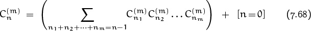
for all integers n?” “If G(z) is a power series that satisfies

what is [zⁿ] G(z)?”

Notice that these are not easy questions. In the ordinary Catalan case (m = 2), we solved (7.69) for G(z) and its coefficients by using the quadratic formula and the binomial theorem; but when m = 3, none of the standard techniques gives any clue about how to solve the cubic equation G = zG³ + 1. So it has turned out to be easier to answer this question before asking it.

Now, however, we know enough to ask even harder questions and deduce their answers. How about this one: “What is [zⁿ] G(z)^l, if l is a positive integer and if G(z) is the power series defined by (7.69)?” The argument we just gave can be used to show that [zⁿ] G(z)^l is the number of sequences of length mn + l with the following three properties:

• Each element is either +1 or (1 – m).

• The partial sums are all positive.

• The total sum is l.

For we get all such sequences in a unique way by putting together l sequences that have the m-Raney property. The number of ways to do this is

Raney proved a generalization of his lemma that tells us how to count such sequences: If x₁, x₂, . . . , x_m is any sequence of integers with x_j ≤ 1 for all j, and with x₁ + x₂ + · · · + x_m = l > 0, then exactly l of the cyclic shifts

x₁, x₂, . . . , x_m, x₂, . . . , x_m, x₁, . . . , x_m, x₁, . . . , x_m–1

have all partial sums positive.

For example, we can check this statement on the sequence –2, 1, –1, 0, 1, 1, –1, 1, 1, 1. The cyclic shifts are

–2, 1, –1, 0, 1, 1, –1, 1, 1, 1		1, –1, 1, 1, 1, –2, 1, –1, 0, 1
1, –1, 0, 1, 1, –1, 1, 1, 1, –2		–1, 1, 1, 1, –2, 1, –1, 0, 1, 1
–1, 0, 1, 1, –1, 1, 1, 1, –2, 1		1, 1, 1, –2, 1, –1, 0, 1, 1, –1  √
0, 1, 1, –1, 1, 1, 1, –2, 1, –1		1, 1, –2, 1, –1, 0, 1, 1, –1, 1
1, 1, –1, 1, 1, 1, –2, 1, –1, 0  √		1, –2, 1, –1, 0, 1, 1, –1, 1, 1

and only the two examples marked ‘√’ have all partial sums positive. This generalized lemma is proved in exercise 13.

A sequence of +1’s and (1 – m)’s that has length mn + l and total sum l must have exactly n occurrences of (1 – m). The generalized lemma tells us that l/(mn + l) of these sequences have all partial sums positive; hence our tough question has a surprisingly simple answer:

for all integers l > 0.

Readers who haven’t forgotten Chapter 5 might well be experiencing déjà vu: “That formula looks familiar; haven’t we seen it before?” Yes, indeed; Lambert’s equation (5.60) says that

Therefore the generating function G(z) in (7.69) must actually be the generalized binomial series . Sure enough, equation (5.59) says

_m(z)^1–m – _m(z)^–m = z ,

which is the same as

_m(z) – 1 = z_m(z)^m .

Let’s switch to the notation of Chapter 5, now that we know we’re dealing with generalized binomials. Chapter 5 stated a bunch of identities without proof. We have now closed part of the gap by proving that the power series defined by

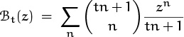
has the remarkable property that

whenever t and r are positive integers.

Can we extend these results to arbitrary values of t and r? Yes; because the coefficients are polynomials in t and r. The general rth power defined by

has coefficients that are polynomials in t and r; and those polynomials are equal to for infinitely many values of t and r. So the two sequences of polynomials must be identically equal.

Chapter 5 also mentions the generalized exponential series

which is said in (5.60) to have an equally remarkable property:

We can prove this as a limiting case of the formulas for _t(z), because it is not difficult to show that

7.6 Exponential GF’s

Sometimes a sequence g_n has a generating function whose properties are quite complicated, while the related sequence g_n/n! has a generating function that’s quite simple. In such cases we naturally prefer to work with g_n/n! and then multiply by n! at the end. This trick works sufficiently often that we have a special name for it: We call the power series

the exponential generating function or “egf” of the sequence g₀, g₁, g₂, . . .. This name arises because the exponential function e^z is the egf of 1, 1, 1, . . ..

Many of the generating functions in Table 351 are actually egf’s. For example, equation (7.50) says that is the egf for the sequence . The ordinary generating function for this sequence is much more complicated (and also divergent).

Exponential generating functions have their own basic maneuvers, analogous to the operations we learned in Section 7.2. For example, if we multiply the egf of g_n by z, we get

this is the egf of 0, g₀, 2g₁, . . . = ng_n–1.

Differentiating the egf of g₀, g₁, g₂, . . . with respect to z gives

Are we having fun yet?

this is the egf of g₁, g₂, . . .. Thus differentiation on egf’s corresponds to the left-shift operation (G(z) – g₀)/z on ordinary gf’s. (We used this left-shift property of egf’s when we studied hypergeometric series, (5.106).) Integration of an egf gives

this is a right shift, the egf of 0, g₀, g₁, . . ..

The most interesting operation on egf’s, as on ordinary gf’s, is multiplication. If and are egf’s for f_n and g_n, then is the egf for a sequence h_n called the binomial convolution of f_n and g_n:

Binomial coefficients appear here because , hence

in other words, h_n/n! is the ordinary convolution of f_n/n! and g_n/n!.

Binomial convolutions occur frequently in applications. For example, we defined the Bernoulli numbers in (6.79) by the implicit recurrence

this can be rewritten as a binomial convolution, if we substitute n for m + 1 and add the term B_n to both sides:

We can now relate this recurrence to power series (as promised in Chapter 6) by introducing the egf for Bernoulli numbers, . The left-hand side of (7.76) is the binomial convolution of B_n with the constant sequence 1, 1, 1, . . . ; hence the egf of the left-hand side is . The egf of the right-hand side is . Therefore we must have ; we have proved equation (6.81), which appears also in Table 351 as equation (7.44).

Now let’s look again at a sum that has been popping up frequently in this book,

This time we will try to analyze the problem with generating functions, in hopes that it will suddenly become simpler. We will consider n to be fixed and m variable; thus our goal is to understand the coefficients of the power series

We know that the generating function for 1, k, k², . . . is

hence

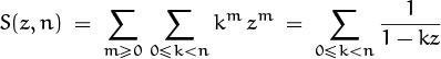
by interchanging the order of summation. We can put this sum in closed form,

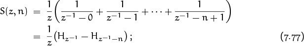
but we know nothing about expanding such a closed form in powers of z.

Exponential generating functions come to the rescue. The egf of our sequence S₀(n), S₁(n), S₂(n), . . . is

To get these coefficients S_m(n) we can use the egf for 1, k, k², . . ., namely

and we have

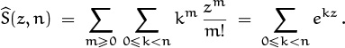
And the latter sum is a geometric progression, so there’s a closed form

Eureka! All we need to do is figure out the coefficients of this relatively simple function, and we’ll know S_m(n), because S_m(n) = m![z^m]Ŝ(z,n).

Here’s where Bernoulli numbers come into the picture. We observed a moment ago that the egf for Bernoulli numbers is

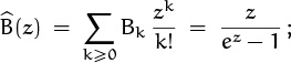
hence we can write

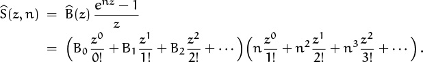
The sum S_m(n) is m! times the coefficient of z^m in this product. For example,

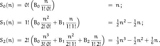
We have therefore derived the formula for the umpteenth time, and this was the simplest derivation of all: In a few lines we have found the general behavior of S_m(n) for all m.

The general formula can be written

where B_m(x) is the Bernoulli polynomial defined by

Here’s why: The Bernoulli polynomial is the binomial convolution of the sequence B₀, B₁, B₂, . . . with 1, x, x², . . . ; hence the exponential generating function for B₀(x), B₁(x), B₂(x), . . . is the product of their egf’s,

Equation (7.79) follows because the egf for 0, S₀(n), 2S₁(n), . . . is, by (7.78),

Let’s turn now to another problem for which egf’s are just the thing: How many spanning trees are possible in the complete graph on n vertices {1, 2, . . . , n}? Let’s call this number t_n. The complete graph has edges, one edge joining each pair of distinct vertices; so we’re essentially looking for the total number of ways to connect up n given things by drawing n – 1 lines between them.

We have t₁ = t₂ = 1. Also t₃ = 3, because a complete graph on three vertices is a fan of order 2; we know that f₂ = 3. And there are sixteen spanning trees when n = 4:

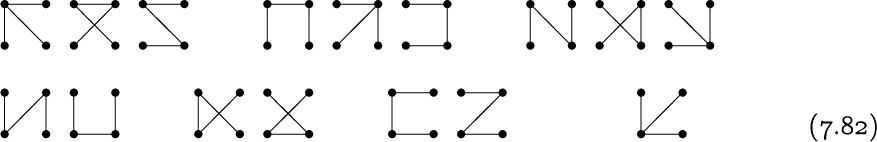
Hence t₄ = 16.

Our experience with the analogous problem for fans suggests that the best way to tackle this problem is to single out one vertex, and to look at the blocks or components that the spanning tree joins together when we ignore all edges that touch the special vertex. If the non-special vertices form m components of sizes k₁, k₂, . . . , k_m, then we can connect them to the special vertex in k₁k₂ . . . k_m ways. For example, in the case n = 4, we can consider the lower left vertex to be special. The top row of (7.82) shows 3t₃ cases where the other three vertices are joined among themselves in t₃ ways and then connected to the lower left in 3 ways. The bottom row shows 2·1 × t₂t₁ × solutions where the other three vertices are divided into components of sizes 2 and 1 in ways; there’s also the case where the other three vertices are completely unconnected among themselves.

This line of reasoning leads to the recurrence

for all n > 1. Here’s why: There are ways to assign n–1 elements to a sequence of m components of respective sizes k₁, k₂, . . . , k_m; there are t_k1 t_k2 . . . t_km ways to connect up those individual components with spanning trees; there are k₁k₂ . . . k_m ways to connect vertex n to those components; and we divide by m! because we want to disregard the order of the components. For example, when n = 4 the recurrence says that

The recurrence for t_n looks formidable at first, possibly even frightening; but it really isn’t bad, only convoluted. We can define

u_n = n t_n

and then everything simplifies considerably:

The inner sum is the coefficient of z^n–1 in the egf (z), raised to the mth power; and we obtain the correct formula also when n = 1, if we add in the term (z)⁰ that corresponds to the case m = 0. So

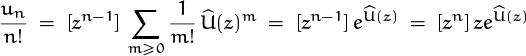
for all n > 0, and we have the equation

Progress! Equation (7.84) is almost like

ℇ(z) = e^{z ℇ(z)} ,

which defines the generalized exponential series ℇ(z) = ℇ₁(z) in (5.59) and (7.71); indeed, we have

(z) = z ℇ (z) .

So we can read off the answer to our problem:

The complete graph on {1, 2, . . . , n} has exactly n^n–2 spanning trees, for all n > 0.

7.7 Dirichlet Generating Functions

There are many other possible ways to generate a sequence from a series; any system of “kernel” functions K_n(z) such that

can be used, at least in principle. Ordinary generating functions use K_n(z) = zⁿ, and exponential generating functions use K_n(z) = zⁿ/n!; we could also try falling factorial powers zⁿ, or binomial coefficients zⁿ/n! = .

The most important alternative to gf’s and egf’s uses the kernel functions 1/n^z; it is intended for sequences g₁, g₂, . . . that begin with n = 1 instead of n = 0:

This is called a Dirichlet generating function (dgf), because the German mathematician Gustav Lejeune Dirichlet (1805–1859) made much of it.

For example, the dgf of the constant sequence 1, 1, 1, . . . is

This is Riemann’s zeta function, which we have also called the generalized harmonic number when z > 1.

The product of Dirichlet generating functions corresponds to a special kind of convolution:

Thus is the dgf of the sequence

For example, we know from (4.55) that ∑_d μ(d) = [n = 1]; this is the Dirichlet convolution of the Möbius sequence μ(1), μ(2), μ(3), . . . with 1, 1, 1, . . . , hence

In other words, the dgf of μ(1), μ(2), μ(3), . . . is ζ(z)^–1 .

Dirichlet generating functions are particularly valuable when the sequence g₁, g₂, . . . is a multiplicative function, namely when

g_mn = g_m g_n           for m ⊥ n.

In such cases the values of g_n for all n are determined by the values of g_n when n is a power of a prime, and we can factor the dgf into a product over primes:

If, for instance, we set g_n = 1 for all n, we obtain a product representation of Riemann’s zeta function:

The Möbius function has μ(p) = –1 and μ(p^k) = 0 for k > 1, hence its dgf is

this agrees, of course, with (7.89) and (7.91). Euler’s φ function has φ(p^k) = p^k – p^k–1, hence its dgf has the factored form

We conclude that (z) = ζ(z – 1)/ζ(z).

Exercises

Warmups

1. An eccentric collector of 2 × n domino tilings pays $4 for each vertical domino and $1 for each horizontal domino. How many tilings are worth exactly $m by this criterion? For example, when m = 6 there are three solutions: , , and .

2. Give the generating function and the exponential generating function for the sequence 2, 5, 13, 35, . . . = 2ⁿ + 3ⁿ in closed form.

3. What is ∑_n≥0 H_n/10ⁿ?

4. The general expansion theorem for rational functions P(z)/Q(z) is not completely general, because it restricts the degree of P to be less than the degree of Q. What happens if P has a larger degree than this?

5. Find a generating function S(z) such that

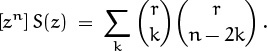
Basics

6. Show that the recurrence (7.32) can be solved by the repertoire method, without using generating functions.

7. Solve the recurrence

8. What is [zⁿ] (ln(1 – z))²/(1 – z)^{m +1}?

9. Use the result of the previous exercise to evaluate .

10. Set r = s = –1/2 in identity (7.62) and then remove all occurrences of 1/2 by using tricks like (5.36). What amazing identity do you deduce?

I deduce that Clark Kent is really Superman.

11. This problem, whose three parts are independent, gives practice in the manipulation of generating functions. We assume that A(z) = ∑_n a_nzⁿ, B(z) = ∑_n b_nzⁿ, C(z) = ∑_n c_nzⁿ, and that the coefficients are zero for negative n.

a. If c_n = ∑_j+2k≤n a_jb_k, express C in terms of A and B.

b. If , express A in terms of B.

c. If r is a real number and if , express A in terms of B; then use your formula to find coefficients f_k(r) such that .

12. How many ways are there to put the numbers {1, 2, . . . , 2n} into a 2 × n array so that rows and columns are in increasing order from left to right and from top to bottom? For example, one solution when n = 5 is

13. Prove Raney’s generalized lemma, which is stated just before (7.70).

14. Solve the recurrence

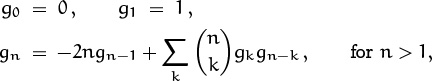
by using an exponential generating function.

15. The Bell number ϖ_n is the number of ways to partition n things into subsets. For example, ϖ₃ = 5 because we can partition {1, 2, 3} in the following ways:

{1, 2, 3};   {1, 2}∪{3};   {1, 3}∪{2};   {1}∪{2, 3};   {1}∪{2}∪{3}.

Prove that , and use this recurrence to find a closed form for the exponential generating function P(z) = ∑_n ϖ_nzⁿ/n!.

16. Two sequences a_n and b_n are related by the convolution formula

also a₀ = 0 and b₀ = 1. Prove that the corresponding generating functions satisfy ln .

17. Show that the exponential generating function Ĝ(z) of a sequence is related to the ordinary generating function G(z) by the formula

if the integral exists.

18. Find the Dirichlet generating functions for the sequences

a.

b. g_n = ln n;

c. g_n = [n is squarefree].

Express your answers in terms of the zeta function. (Squarefreeness is defined in exercise 4.13.)

19. Every power series F(z) = ∑_n≥0 f_nzⁿ with f₀ = 1 defines a sequence of polynomials f_n(x) by the rule

where f_n(1) = f_n and f_n(0) = [n = 0]. In general, f_n(x) has degree n. Show that such polynomials always satisfy the convolution formulas

What do you mean, “in general”? If f₁ = f₂ = · · · = f_m–1 = 0, the degree of f_n(x) is at most n/m .

(The identities in Tables 202 and 272 are special cases of this trick.)

20. A power series G(z) is called differentiably finite if there exist finitely many polynomials P₀(z), . . . , P_m(z), not all zero, such that

P₀(z)G(z) + P₁(z)G′(z) + · · · + P_m(z)G^(m)(z) = 0 .

A sequence of numbers g₀, g₁, g₂, . . . is called polynomially recursive if there exist finitely many polynomials p₀(z), . . . , p_m(z), not all zero, such that

p₀(n)g_n + p₁(n)g_n+1 + · · · + p_m(n)g_n+m = 0

for all integers n ≥ 0. Prove that a generating function is differentiably finite if and only if its sequence of coefficients is polynomially recursive.

Homework exercises

21. A robber holds up a bank and demands $500 in tens and twenties. He also demands to know the number of ways in which the cashier can give him the money. Find a generating function G(z) for which this number is [z⁵⁰⁰] G(z), and a more compact generating function (z) for which this number is [z⁵⁰] (z). Determine the required number of ways by (a) using partial fractions; (b) using a method like (7.39).

Will he settle for 2 × n domino tilings?

22. Let P be the sum of all ways to “triangulate” polygons:

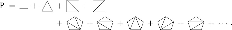
(The first term represents a degenerate polygon with only two vertices; every other term shows a polygon that has been divided into triangles. For example, a pentagon can be triangulated in five ways.) Define a “multiplication” operation AΔB on triangulated polygons A and B so that the equation

P = __ + P△P

is valid. Then replace each triangle by ‘z’; what does this tell you about the number of ways to decompose an n-gon into triangles?

23. In how many ways can a 2 × 2 × n pillar be built out of 2 × 1 × 1 bricks?

At union rates, as many as you can afford, plus a few.

24. How many spanning trees are in an n-wheel (a graph with n “outer” vertices in a cycle, each connected to an (n + 1)st “hub” vertex), when n ≥ 3?

25. Let m ≥ 2 be an integer. What is a closed form for the generating function of the sequence n mod m, as a function of z and m? Use this generating function to express ‘n mod m’ in terms of the complex number ω = e^2πi/m. (For example, when m = 2 we have ω = –1 and n mod .)

26. The second-order Fibonacci numbers are defined by the recurrence

Express in terms of the usual Fibonacci numbers F_n and F_n+1.

27. A 2 × n domino tiling can also be regarded as a way to draw n disjoint lines in a 2 × n array of points:

If we superimpose two such patterns, we get a set of cycles, since every point is touched by two lines. For example, if the lines above are combined with the lines

the result is

The same set of cycles is also obtained by combining

But we get a unique way to reconstruct the original patterns from the superimposed ones if we assign orientations to the vertical lines by using arrows that go alternately up/down/up/down/· · · in the first pattern and alternately down/up/down/up/· · · in the second. For example,

The number of such oriented cycle patterns must therefore be , and we should be able to prove this via algebra. Let Q_n be the number of oriented 2 × n cycle patterns. Find a recurrence for Q_n, solve it with generating functions, and deduce algebraically that .

28. The coefficients of A(z) in (7.39) satisfy A_r+A_r+10+A_r+20+A_r+30 = 100 for 0 ≤ r < 10. Find a “simple” explanation for this.

29. What is the sum of Fibonacci products

30. If the generating function G(z) = 1/(1 – αz)(1 – βz) has the partial fraction decomposition a/(1–αz)+b/(1–βz), what is the partial fraction decomposition of G(z)ⁿ?

31. What function g(n) of the positive integer n satisfies the recurrence

where φ is Euler’s totient function?

32. An arithmetic progression is an infinite set of integers

{an + b} = {b, a + b, 2a + b, 3a + b, . . . } .

A set of arithmetic progressions {a₁n + b₁}, . . . , {a_mn + b_m} is called an exact cover if every nonnegative integer occurs in one and only one of the progressions. For example, the three progressions {2n}, {4n + 1}, {4n + 3} constitute an exact cover. Show that if {a₁n + b₁}, . . . , {a_mn + b_m} is an exact cover such that 2 ≤ a₁ ≤ · · · ≤ a_m, then a_m–1 = a_m. Hint: Use generating functions.

Exam problems

33. What is [w^mzⁿ] (ln(1 + z))/(1 – wz)?

34. Find a closed form for the generating function ∑_n≥0 G_n(z)wⁿ, if

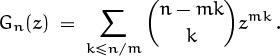
(Here m is a fixed positive integer.)

35. Evaluate the sum ∑_0<k<n 1/k(n – k) in two ways:

a. Expand the summand in partial fractions.

b. Treat the sum as a convolution and use generating functions.

36. Let A(z) be the generating function for a₀, a₁, a₂, a₃, . . . . Express ∑_n a_n/mzⁿ in terms of A, z, and m.

37. Let a_n be the number of ways to write the positive integer n as a sum of powers of 2, disregarding order. For example, a₄ = 4, since 4 = 2 + 2 = 2 + 1 + 1 = 1 + 1 + 1 + 1. By convention we let a₀ = 1. Let be the cumulative sum of the first a’s.

a. Make a table of the a’s and b’s up through n = 10. What amazing relation do you observe in your table? (Don’t prove it yet.)

b. Express the generating function A(z) as an infinite product.

c. Use the expression from part (b) to prove the result of part (a).

38. Find a closed form for the double generating function

Generalize your answer to obtain, for fixed m ≥ 2, a closed form for

39. Given positive integers m and n, find closed forms for

(For example, when m = 2 and n = 3 the sums are 1·2 + 1·3 + 2·3 and 1·1+1·2+1·3+2·2+2·3+3·3.) Hint: What are the coefficients of z^m in the generating functions (1 + a₁z) . . . (1 + a_nz) and 1/(1 – a₁z) . . . (1 – a_nz)?

40. Express in closed form.

41. An up-down permutation of order n is an arrangement a₁a₂ . . . a_n of the integers {1, 2, . . . , n} that goes alternately up and down:

a₁ < a₂ > a₃ < a₄ > · · · .

For example, 35142 is an up-down permutation of order 5. If A_n denotes the number of up-down permutations of order n, show that the exponential generating function of A_n is (1 + sin z)/cos z.

42. A space probe has discovered that organic material on Mars has DNA composed of five symbols, denoted by (a, b, c, d, e), instead of the four components in earthling DNA. The four pairs cd, ce, ed, and ee never occur consecutively in a string of Martian DNA, but any string without forbidden pairs is possible. (Thus bbcda is forbidden but bbdca is OK.) How many Martian DNA strings of length n are possible? (When n = 2 the answer is 21, because the left and right ends of a string are distinguishable.)

43. The Newtonian generating function of a sequence g_n is defined to be

Find a convolution formula that defines the relation between sequences f_n, g_n, and h_n whose Newtonian generating functions are related by the equation . Try to make your formula as simple and symmetric as possible.

44. Let q_n be the number of possible outcomes when n numbers {x₁, . . . , x_n} are compared with each other. For example, q₃ = 13 because the possibilities are

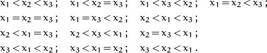
Find a closed form for the egf (z) = Σ_n q_nzⁿ/n!. Also find sequences a_n, b_n, c_n such that

45. Evaluate ∑_m,n>0^{[m ⊥ n]/m2n2.}

46. Evaluate

in closed form. Hint: .

47. Show that the numbers U_n and V_n of 3 × n domino tilings, as given in (7.34), are closely related to the fractions in the Stern–Brocot tree that converge to .

48. A certain sequence g_n satisfies the recurrence

ag_n + bg_n+1 + cg_n+2 + d = 0 ,        integer n ≥ 0,

for some integers (a, b, c, d) with gcd(a, b, c, d) = 1. It also has the closed form

g_n = α(1 + )ⁿ ,       integer n ≥ 0,

for some real number α between 0 and 1. Find a, b, c, d, and α.

49. This is a problem about powers and parity.

Kissinger, take note.

a. Consider the sequence a₀, a₁, a₂, . . . = 2, 2, 6, . . . defined by the formula

a_n = (1 + )ⁿ + (1 – )ⁿ .

Find a simple recurrence relation that is satisfied by this sequence.

b. Prove that (1 + )ⁿ ≡ n (mod 2) for all integers n > 0.

c. Find a number α of the form , where p and q are positive integers, such that αⁿ ≡ n (mod 2) for all integers n > 0.

Bonus problems

50. Continuing exercise 22, consider the sum of all ways to decompose polygons into polygons:

Find a symbolic equation for Q and use it to find a generating function for the number of ways to draw nonintersecting diagonals inside a convex n-gon. (Give a closed form for the generating function as a function of z; you need not find a closed form for the coefficients.)

51. Prove that the product

is the generating function for tilings of an m×n rectangle with dominoes. (There are mn factors, which we can imagine are written in the mn cells of the rectangle. If mn is odd, the middle factor is zero. The coefficient of is the number of ways to do the tiling with j vertical and k horizontal dominoes.) Hint: This is a difficult problem, really beyond the scope of this book. You may wish to simply verify the formula in the case m = 3, n = 4.

Is this a hint or a warning?

52. Prove that the polynomials defined by the recurrence

have the form , where is a positive integer for 1 ≤ m ≤ n. Hint: This exercise is very instructive but not very easy.

53. The sequence of pentagonal numbers 1, 5, 12, 22, . . . generalizes the triangular and square numbers in an obvious way:

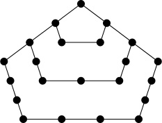
Let the nth triangular number be T_n = n(n+1)/2; let the nth pentagonal number be P_n = n(3n – 1)/2; and let U_n be the 3 × n domino-tiling number defined in (7.38). Prove that the triangular number T_{(U4n+2–1)/2} is also a pentagonal number. Hint: .

54. Consider the following curious construction:

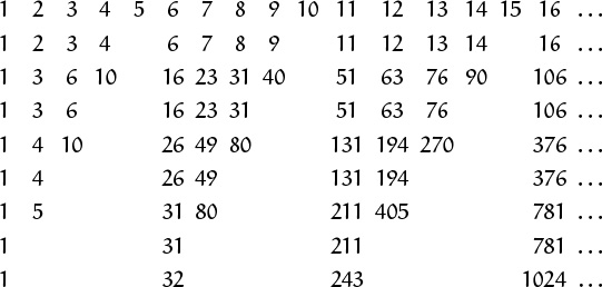
(Start with a row containing all the positive integers. Then delete every mth column; here m = 5. Then replace the remaining entries by partial sums. Then delete every (m – 1)st column. Then replace with partial sums again, and so on.) Use generating functions to show that the final result is the sequence of mth powers. For example, when m = 5 we get 1⁵, 2⁵, 3⁵, 4⁵, . . . as shown.

55. Prove that if the power series F(z) and G(z) are differentiably finite (as defined in exercise 20), then so are F(z) + G(z) and F(z)G(z).

Research problems

56. Prove that there is no “simple closed form” for the coefficient of zⁿ in (1 + z + z²)ⁿ, as a function of n, in some large class of “simple closed forms.”

57. Prove or disprove: If all the coefficients of G(z) are either 0 or 1, and if all the coefficients of G(z)² are less than some constant M, then infinitely many of the coefficients of G(z)² are zero.