4. Number Theory
Integers are central to the discrete mathematics we are emphasizing in this book. Therefore we want to explore the theory of numbers, an important branch of mathematics concerned with the properties of integers.
We tested the number theory waters in the previous chapter, by introducing binary operations called ‘mod’ and ‘gcd’. Now let’s plunge in and really immerse ourselves in the subject.
In other words, be prepared to drown.
4.1 Divisibility
We say that m divides n (or n is divisible by m) if m > 0 and the ratio n/m is an integer. This property underlies all of number theory, so it’s convenient to have a special notation for it. We therefore write
(The notation ‘m|n’ is actually much more common than ‘mn’ in current mathematics literature. But vertical lines are overused—for absolute values, set delimiters, conditional probabilities, etc.—and backward slashes are underused. Moreover, ‘mn’ gives an impression that m is the denominator of an implied ratio. So we shall boldly let our divisibility symbol lean leftward.)
If m does not divide n we write ‘![]() ’.
’.
There’s a similar relation, “n is a multiple of m,” which means almost the same thing except that m doesn’t have to be positive. In this case we simply mean that n = mk for some integer k. Thus, for example, there’s only one multiple of 0 (namely 0), but nothing is divisible by 0. Every integer is a multiple of –1, but no integer is divisible by –1 (strictly speaking). These definitions apply when m and n are any real numbers; for example, 2π is divisible by π. But we’ll almost always be using them when m and n are integers. After all, this is number theory.
“. . . no integer is divisible by –1 (strictly speaking).”
—Graham, Knuth, and Patashnik [161]
The greatest common divisor of two integers m and n is the largest integer that divides them both:
In Britain we call this ‘hcf’ (highest common factor).
For example, gcd(12, 18) = 6. This is a familiar notion, because it’s the common factor that fourth graders learn to take out of a fraction m/n when reducing it to lowest terms: 12/18 = (12/6)/(18/6) = 2/3. Notice that if n > 0 we have gcd(0, n) = n, because any positive number divides 0, and because n is the largest divisor of itself. The value of gcd(0, 0) is undefined.
Another familiar notion is the least common multiple,
Not to be confused with the greatest common multiple.
this is undefined if m ≤ 0 or n ≤ 0. Students of arithmetic recognize this as the least common denominator, which is used when adding fractions with denominators m and n. For example, lcm(12, 18) = 36, and fourth graders know that ![]() . The lcm is somewhat analogous to the gcd, but we don’t give it equal time because the gcd has nicer properties.
. The lcm is somewhat analogous to the gcd, but we don’t give it equal time because the gcd has nicer properties.
One of the nicest properties of the gcd is that it is easy to compute, using a 2300-year-old method called Euclid’s algorithm. To calculate gcd(m, n), for given values 0 ≤ m < n, Euclid’s algorithm uses the recurrence

Thus, for example, gcd(12, 18) = gcd(6, 12) = gcd(0, 6) = 6. The stated recurrence is valid, because any common divisor of m and n must also be a common divisor of both m and the number n mod m, which is n – ![]() n/m
n/m![]() m. There doesn’t seem to be any recurrence for lcm(m, n) that’s anywhere near as simple as this. (See exercise 2.)
m. There doesn’t seem to be any recurrence for lcm(m, n) that’s anywhere near as simple as this. (See exercise 2.)
Euclid’s algorithm also gives us more: We can extend it so that it will compute integers m′ and n′ satisfying
(Remember that m′ or n′ can be negative.)
Here’s how. If m = 0, we simply take m′ = 0 and n′ = 1. Otherwise we let r = n mod m and apply the method recursively with r and m in place of m and n, computing ![]() and
and ![]() such that
such that
Since r = n – ![]() n/m
n/m![]() m and gcd(r, m) = gcd(m, n), this equation tells us that
m and gcd(r, m) = gcd(m, n), this equation tells us that
The left side can be rewritten to show its dependency on m and n:
hence ![]() and n′ =
and n′ = ![]() are the integers we need in (4.5). For example, in our favorite case m = 12, n = 18, this method gives 6 = 0·0+1·6 = 1·6 + 0·12 = (–1)·12 + 1·18.
are the integers we need in (4.5). For example, in our favorite case m = 12, n = 18, this method gives 6 = 0·0+1·6 = 1·6 + 0·12 = (–1)·12 + 1·18.
But why is (4.5) such a neat result? The main reason is that there’s a sense in which the numbers m′ and n′ actually prove that Euclid’s algorithm has produced the correct answer in any particular case. Let’s suppose that our computer has told us after a lengthy calculation that gcd(m, n) = d and that m′m + n′n = d; but we’re skeptical and think that there’s really a greater common divisor, which the machine has somehow overlooked. This cannot be, however, because any common divisor of m and n has to divide m′m + n′n; so it has to divide d; so it has to be ≤ d. Furthermore we can easily check that d does divide both m and n. (Algorithms that output their own proofs of correctness are called self-certifying.)
We’ll be using (4.5) a lot in the rest of this chapter. One of its important consequences is the following mini-theorem:
(Proof: If k divides both m and n, it divides m′m + n′n, so it divides gcd(m, n). Conversely, if k divides gcd(m, n), it divides a divisor of m and a divisor of n, so it divides both m and n.) We always knew that any common divisor of m and n must be less than or equal to their gcd; that’s the definition of greatest common divisor. But now we know that any common divisor is, in fact, a divisor of their gcd.
Sometimes we need to do sums over all divisors of n. In this case it’s often useful to use the handy rule
which holds since n/m runs through all divisors of n when m does. For example, when n = 12 this says that a1 + a2 + a3 + a4 + a6 + a12 = a12 + a6 + a4 + a3 + a2 + a1.
There’s also a slightly more general identity,
which is an immediate consequence of the definition (4.1). If n is positive, the right-hand side of (4.8) is ∑k an/k; hence (4.8) implies (4.7). And equation (4.8) works also when n is negative. (In such cases, the nonzero terms on the right occur when k is the negative of a divisor of n.)
Moreover, a double sum over divisors can be “interchanged” by the law
For example, this law takes the following form when n = 12:
a1,1 + (a1,2 + a2,2) + (a1,3 + a3,3)
+ (a1,4 + a2,4 + a4,4) + (a1,6 + a2,6 + a3,6 + a6,6)
+ (a1,12 + a2,12 + a3,12 + a4,12 + a6,12 + a12,12)
= (a1,1 + a1,2 + a1,3 + a1,4 + a1,6 + a1,12)
+ (a2,2 + a2,4 + a2,6 + a2,12) + (a3,3 + a3,6 + a3,12)
+ (a4,4 + a4,12) + (a6,6 + a6,12) + a12,12 .
We can prove (4.9) with Iversonian manipulation. The left-hand side is
the right-hand side is
which is the same except for renaming the indices. This example indicates that the techniques we’ve learned in Chapter 2 will come in handy as we study number theory.
4.2 Primes
A positive integer p is called prime if it has just two divisors, namely 1 and p. Throughout the rest of this chapter, the letter p will always stand for a prime number, even when we don’t say so explicitly. By convention, 1 isn’t prime, so the sequence of primes starts out like this:
2, 3, 5, 7, 11, 13, 17, 19, 23, 29, 31, 37, 41, . . . .
How about the p in ‘explicitly’?
Some numbers look prime but aren’t, like 91 (= 7 · 13) and 161 (= 7 · 23). These numbers, and others that have nontrivial divisors, are called composite. Every integer greater than 1 is either prime or composite, but not both.
Primes are of great importance, because they’re the fundamental building blocks of all the positive integers. Any positive integer n can be written as a product of primes,

For example, 12 = 2 · 2 · 3; 11011 = 7 · 11 · 11 · 13; 11111 = 41 · 271. (Products denoted by Π are analogous to sums denoted by ∑, as explained in exercise 2.25. If m = 0, we consider this to be an empty product, whose value is 1 by definition; that’s the way n = 1 gets represented by (4.10).) Such a factorization is always possible because if n > 1 is not prime it has a divisor n1 such that 1 < n1 < n; thus we can write n = n1 · n2, and (by induction) we know that n1 and n2 can be written as products of primes.
Moreover, the expansion in (4.10) is unique: There’s only one way to write n as a product of primes in nondecreasing order. This statement is called the Fundamental Theorem of Arithmetic, and it seems so obvious that we might wonder why it needs to be proved. How could there be two different sets of primes with the same product? Well, there can’t, but the reason isn’t simply “by definition of prime numbers.” For example, if we consider the set of all real numbers of the form ![]() when m and n are integers, the product of any two such numbers is again of the same form, and we can call such a number “prime” if it can’t be factored in a nontrivial way. The number 6 has two representations,
when m and n are integers, the product of any two such numbers is again of the same form, and we can call such a number “prime” if it can’t be factored in a nontrivial way. The number 6 has two representations, ![]() ; yet exercise 36 shows that 2, 3,
; yet exercise 36 shows that 2, 3, ![]() , and
, and ![]() are all “prime” in this system.
are all “prime” in this system.
Therefore we should prove rigorously that (4.10) is unique. There is certainly only one possibility when n = 1, since the product must be empty in that case; so let’s suppose that n > 1 and that all smaller numbers factor uniquely. Suppose we have two factorizations
n = p1 . . . pm = q1 . . . qk , p1≤ · · · ≤pm and q1≤ · · · ≤qk,
where the p’s and q’s are all prime. We will prove that p1 = q1. If not, we can assume that p1 < q1, making p1 smaller than all the q’s. Since p1 and q1 are prime, their gcd must be 1; hence Euclid’s self-certifying algorithm gives us integers a and b such that ap1 + bq1 = 1. Therefore
ap1q2 . . . qk + bq1q2 . . . qk = q2 . . . qk .
Now p1 divides both terms on the left, since q1q2 . . . qk = n; hence p1 divides the right-hand side, q2 . . . qk. Thus q2 . . . qk/p1 is an integer, and q2 . . . qk has a prime factorization in which p1 appears. But q2 . . . qk < n, so it has a unique factorization (by induction). Hence p1 must be either q2 or · · · or qn; yet p1 is strictly smaller! This contradiction shows that p1 must be equal to q1 after all. Therefore we can divide both of n’s factorizations by p1, obtaining p2 . . . pm = q2 . . . qk < n. The other factors must likewise be equal (by induction), so our proof of uniqueness is complete.
Sometimes it’s more useful to state the Fundamental Theorem in another way: Every positive integer can be written uniquely in the form
It’s the factorization, not the theorem, that’s unique.
The right-hand side is a product over infinitely many primes; but for any particular n all but a few exponents are zero, so the corresponding factors are 1. Therefore it’s really a finite product, just as many “infinite” sums are really finite because their terms are mostly zero.
Formula (4.11) represents n uniquely, so we can think of the sequence ![]() n2, n3, n5, . . .
n2, n3, n5, . . . ![]() as a number system for positive integers. For example, the prime-exponent representation of 12 is
as a number system for positive integers. For example, the prime-exponent representation of 12 is ![]() 2, 1, 0, 0, . . .
2, 1, 0, 0, . . . ![]() and the prime-exponent representation of 18 is
and the prime-exponent representation of 18 is ![]() 1, 2, 0, 0, . . .
1, 2, 0, 0, . . . ![]() . To multiply two numbers, we simply add their representations. In other words,
. To multiply two numbers, we simply add their representations. In other words,
This implies that
and it follows immediately that
For example, since 12 = 22 ·31 and 18 = 21 ·32, we can get their gcd and lcm by taking the min and max of common exponents:
gcd(12, 18) = 2min(2,1) · 3min(1,2) = 21 ·31 = 6;
lcm(12, 18) = 2max(2,1) · 3max(1,2) = 22 ·32 = 36 .
If the prime p divides a product mn then it divides either m or n, perhaps both, because of the unique factorization theorem. But composite numbers do not have this property. For example, the nonprime 4 divides 60 = 6 · 10, but it divides neither 6 nor 10. The reason is simple: In the factorization 60 = 6 · 10 = (2 · 3)(2 · 5), the two prime factors of 4 = 2 · 2 have been split into two parts, hence 4 divides neither part. But a prime is unsplittable, so it must divide one of the original factors.
4.3 Prime Examples
How many primes are there? A lot. In fact, infinitely many. Euclid proved this long ago in his Theorem 9 : 20, as follows. Consider any finite set of primes, say {P1, P2, . . . , Pk}. Then, said Euclid, we should think about the number

—Euclid [98]
M = P1 · P2 · . . . · Pk + 1.
[Translation: “There are more primes than in any given set of primes.”]
None of the k primes can divide M, because each divides M – 1. Thus there must be some other prime that divides M; perhaps M itself is prime. Every finite set of prime numbers must therefore be incomplete.
Euclid’s proof suggests that we define Euclid numbers by the recurrence
The sequence starts out
e1 = 1 + 1 = 2;
e2 = 2 + 1 = 3;
e3 = 2·3 + 1 = 7;
e4 = 2·3·7 + 1 = 43;
these are all prime. But the next case, e5, is 1807 = 13·139. It turns out that e6 = 3263443 is prime, while
e7 = 547·607·1033·31051;
e8 = 29881·67003·9119521·6212157481 .
It is known that e9, . . . , e17 are composite, and the remaining en are probably composite as well. However, the Euclid numbers are all relatively prime to each other; that is,
gcd(em, en) = 1, when m ≠ n.
Euclid’s algorithm (what else?) tells us this in three short steps, because en mod em = 1 when n > m:
gcd(em, en) = gcd(1, em) = gcd(0, 1) = 1.
Therefore, if we let qj be the smallest prime factor of ej for all j ≥ 1, we get a sequence q1, q2, q3, . . . of infinitely many distinct primes.
Let’s pause to consider the Euclid numbers from the standpoint of Chapter 1. Can we express en in closed form? Recurrence (4.16) can be simplified by removing the three dots: If n > 1 we have
en = e1 . . . en–2en–1 + 1 = (en–1 – 1)en–1 + 1 = ![]() – en–1 + 1 .
– en–1 + 1 .
Thus en has about twice as many decimal digits as en–1. Exercise 37 proves that there’s a constant E ≈ 1.264 such that
And exercise 60 provides a similar formula that gives nothing but primes:
for some constant P. But equations like (4.17) and (4.18) cannot really be considered to be in closed form, because the constants E and P are computed from the numbers en and pn in a sort of sneaky way. No independent relation is known (or likely) that would connect them with other constants of mathematical interest.
Indeed, nobody knows any useful formula that gives arbitrarily large primes but only primes. Computer scientists at Chevron Geosciences did, however, strike mathematical oil in 1984. Using a program developed by David Slowinski, they discovered the largest prime known at that time,
2216091 – 1,
while testing a new Cray X-MP supercomputer. It’s easy to compute this number in a few milliseconds on a personal computer, because modern computers work in binary notation and this number is simply (11 . . . 1)2. All 216,091 of its bits are ‘1’. But it’s much harder to prove that this number is prime. In fact, just about any computation with it takes a lot of time, because it’s so large. For example, even a sophisticated algorithm requires several minutes just to convert 2216091 – 1 to radix 10 on a PC. When printed out, its 65,050 decimal digits require 78 cents U.S. postage to mail first class.
Or probably more, by the time you read this.
Incidentally, 2216091 – 1 is the number of moves necessary to solve the Tower of Hanoi problem when there are 216,091 disks. Numbers of the form
2p – 1
(where p is prime, as always in this chapter) are called Mersenne numbers, after Father Marin Mersenne who investigated some of their properties in the seventeenth century [269]. The Mersenne primes known prior to 1998 occur for p = 2, 3, 5, 7, 13, 17, 19, 31, 61, 89, 107, 127, 521, 607, 1279, 2203, 2281, 3217, 4253, 4423, 9689, 9941, 11213, 19937, 21701, 23209, 44497, 86243, 110503, 132049, 216091, 756839, 859433, 1257787, 1398269, and 2976221.
The number 2n – 1 can’t possibly be prime if n is composite, because 2km – 1 has 2m – 1 as a factor:
2km – 1 = (2m – 1)(2m (k–1) + 2m(k–2) + · · · + 1) .
But 2p – 1 isn’t always prime when p is prime; 211 – 1 = 2047 = 23·89 is the smallest such nonprime. (Mersenne knew this.)
Factoring and primality testing of large numbers are hot topics nowadays. A summary of what was known up to 1981 appears in Section 4.5.4 of [208], and many new results continue to be discovered. Pages 391–394 of that book explain a special way to test Mersenne numbers for primality.
For most of the last five hundred years, the largest known prime has been a Mersenne prime, although only a few dozen Mersenne primes are known. Many people are trying to find larger ones, but it’s getting tough. So those really interested in fame (if not fortune) and a spot in The Guinness Book of World Records might instead try numbers of the form 2nk + 1, for small values of k like 3 or 5. These numbers can be tested for primality almost as quickly as Mersenne numbers can; exercise 4.5.4–27 of [208] gives the details.
We haven’t fully answered our original question about how many primes there are. There are infinitely many, but some infinite sets are “denser” than others. For instance, among the positive integers there are infinitely many even numbers and infinitely many perfect squares, yet in several important senses there are more even numbers than perfect squares. One such sense looks at the size of the nth value. The nth even integer is 2n and the nth perfect square is n2; since 2n is much less than n2 for large n, the nth even integer occurs much sooner than the nth perfect square, so we can say there are many more even integers than perfect squares. A similar sense looks at the number of values not exceeding x. There are ![]() x/2
x/2![]() such even integers and
such even integers and ![]() such perfect squares; since x/2 is much larger than
such perfect squares; since x/2 is much larger than ![]() for large x, again we can say there are many more even integers.
for large x, again we can say there are many more even integers.
Weird. I thought there were the same number of even integers as perfect squares, since there’s a one-to-one correspondence between them.
What can we say about the primes in these two senses? It turns out that the nth prime, Pn, is about n times the natural log of n:
Pn ∼ n ln n.
(The symbol ‘∼’ can be read “is asymptotic to”; it means that the limit of the ratio Pn/n ln n is 1 as n goes to infinity.) Similarly, for the number of primes π(x) not exceeding x we have what’s known as the prime number theorem:
Proving these two facts is beyond the scope of this book, although we can show easily that each of them implies the other. In Chapter 9 we will discuss the rates at which functions approach infinity, and we’ll see that the function n ln n, our approximation to Pn, lies between 2n and n2 asymptotically. Hence there are fewer primes than even integers, but there are more primes than perfect squares.
These formulas, which hold only in the limit as n or x → ∞, can be replaced by more exact estimates. For example, Rosser and Schoenfeld [312] have established the handy bounds
If we look at a “random” integer n, the chances of its being prime are about one in ln n. For example, if we look at numbers near 1016, we’ll have to examine about 16 ln 10 ≈ 36.8 of them before finding a prime. (It turns out that there are exactly 10 primes between 1016 – 370 and 1016 – 1.) Yet the distribution of primes has many irregularities. For example, all the numbers between P1P2 . . . Pn + 2 and P1P2 . . . Pn + Pn+1 – 1 inclusive are composite. Many examples of “twin primes” p and p + 2 are known (5 and 7, 11 and 13, 17 and 19, 29 and 31, . . . , 9999999999999641 and 9999999999999643, . . . ), yet nobody knows whether or not there are infinitely many pairs of twin primes. (See Hardy and Wright [181, §1.4 and §2.8].)
One simple way to calculate all π(x) primes ≤ x is to form the so-called sieve of Eratosthenes: First write down all integers from 2 through x. Next circle 2, marking it prime, and cross out all other multiples of 2. Then repeatedly circle the smallest uncircled, uncrossed number and cross out its other multiples. When everything has been circled or crossed out, the circled numbers are the primes. For example when x = 10 we write down 2 through 10, circle 2, then cross out its multiples 4, 6, 8, and 10. Next 3 is the smallest uncircled, uncrossed number, so we circle it and cross out 6 and 9. Now 5 is smallest, so we circle it and cross out 10. Finally we circle 7. The circled numbers are 2, 3, 5, and 7; so these are the π(10) = 4 primes not exceeding 10.
“Je me sers de la notation très simple n! pour désigner le produit de nombres décroissans depuis n jusqu’à l’unité, savoir n(n – 1) (n – 2) . . . . 3. 2. 1. L’emploi continuel de l’analyse combinatoire que je fais dans la plupart de mes démonstrations, a rendu cette notation indispensable.”
—Ch. Kramp [228]
4.4 Factorial Factors
Now let’s take a look at the factorization of some interesting highly composite numbers, the factorials:

According to our convention for an empty product, this defines 0! to be 1. Thus n! = (n – 1)! n for every positive integer n. This is the number of permutations of n distinct objects. That is, it’s the number of ways to arrange n things in a row: There are n choices for the first thing; for each choice of first thing, there are n – 1 choices for the second; for each of these n(n – 1) choices, there are n – 2 for the third; and so on, giving n(n – 1)(n – 2) . . . (1) arrangements in all. Here are the first few values of the factorial function.
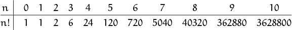
It’s useful to know a few factorial facts, like the first six or so values, and the fact that 10! is about ![]() million plus change; another interesting fact is that the number of digits in n! exceeds n when n ≥ 25.
million plus change; another interesting fact is that the number of digits in n! exceeds n when n ≥ 25.
We can prove that n! is plenty big by using something like Gauss’s trick of Chapter 1:
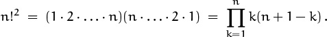
We have ![]() , since the quadratic polynomial
, since the quadratic polynomial ![]() has its smallest value at k = 1 and at k = n, while it has its largest value at
has its smallest value at k = 1 and at k = n, while it has its largest value at ![]() . Therefore
. Therefore
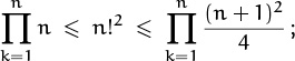
that is,
This relation tells us that the factorial function grows exponentially!!
To approximate n! more accurately for large n we can use Stirling’s formula, which we will derive in Chapter 9:
And a still more precise approximation tells us the asymptotic relative error: Stirling’s formula undershoots n! by a factor of about 1/(12n). Even for fairly small n this more precise estimate is pretty good. For example, Stirling’s approximation (4.23) gives a value near 3598696 when n = 10, and this is about 0.83% ≈ 1/120 too small. Good stuff, asymptotics.
But let’s get back to primes. We’d like to determine, for any given prime p, the largest power of p that divides n!; that is, we want the exponent of p in n!’s unique factorization. We denote this number by ![]() p(n!), and we start our investigations with the small case p = 2 and n = 10. Since 10! is the product of ten numbers,
p(n!), and we start our investigations with the small case p = 2 and n = 10. Since 10! is the product of ten numbers, ![]() 2(10!) can be found by summing the powers-of-2 contributions of those ten numbers; this calculation corresponds to summing the columns of the following array:
2(10!) can be found by summing the powers-of-2 contributions of those ten numbers; this calculation corresponds to summing the columns of the following array:
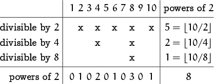
A powerful ruler.
(The column sums form what’s sometimes called the ruler function ρ(k), because of their similarity to ‘![]() ’, the lengths of lines marking fractions of an inch.) The sum of these ten sums is 8; hence 28 divides 10! but 29 doesn’t.
’, the lengths of lines marking fractions of an inch.) The sum of these ten sums is 8; hence 28 divides 10! but 29 doesn’t.
There’s also another way: We can sum the contributions of the rows. The first row marks the numbers that contribute a power of 2 (and thus are divisible by 2); there are ![]() 10/2
10/2![]() = 5 of them. The second row marks those that contribute an additional power of 2; there are
= 5 of them. The second row marks those that contribute an additional power of 2; there are ![]() 10/4
10/4![]() = 2 of them. And the third row marks those that contribute yet another; there are
= 2 of them. And the third row marks those that contribute yet another; there are ![]() 10/8
10/8![]() = 1 of them. These account for all contributions, so we have
= 1 of them. These account for all contributions, so we have ![]() 2(10!) = 5 + 2 + 1 = 8.
2(10!) = 5 + 2 + 1 = 8.
For general n this method gives

This sum is actually finite, since the summand is zero when 2k > n. Therefore it has only ![]() lg n
lg n![]() nonzero terms, and it’s computationally quite easy. For instance, when n = 100 we have
nonzero terms, and it’s computationally quite easy. For instance, when n = 100 we have
![]() 2(100!) = 50 + 25 + 12 + 6 + 3 + 1 = 97.
2(100!) = 50 + 25 + 12 + 6 + 3 + 1 = 97.
Each term is just the floor of half the previous term. This is true for all n, because as a special case of (3.11) we have ![]() n/2k+1
n/2k+1![]() =
= ![]()
![]() n/2k
n/2k![]() /2
/2![]() . It’s especially easy to see what’s going on here when we write the numbers in binary:
. It’s especially easy to see what’s going on here when we write the numbers in binary:
| 100 = | (1100100)2 = | 100 |
| (110010)2 = | 50 | |
| (11001)2 = | 25 | |
| (1100)2 = | 12 | |
| (110)2 = | 6 | |
| (11)2 = | 3 | |
| (1)2 = | 1 |
We merely drop the least significant bit from one term to get the next.
The binary representation also shows us how to derive another formula,
where ν2(n) is the number of 1’s in the binary representation of n. This simplification works because each 1 that contributes 2m to the value of n contributes 2m–1 + 2m–2 + · · · + 20 = 2m – 1 to the value of ![]() 2(n!).
2(n!).
Generalizing our findings to an arbitrary prime p, we have

by the same reasoning as before.
About how large is ![]() p(n!)? We get an easy (but good) upper bound by simply removing the floor from the summand and then summing an infinite geometric progression:
p(n!)? We get an easy (but good) upper bound by simply removing the floor from the summand and then summing an infinite geometric progression:
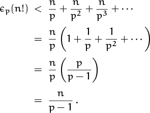
For p = 2 and n = 100 this inequality says that 97 < 100. Thus the upper bound 100 is not only correct, it’s also close to the true value 97. In fact, the true value n – ν2(n) is ∼ n in general, because ν2(n) ≤ ![]() lg n
lg n![]() is asymptotically much smaller than n.
is asymptotically much smaller than n.
When p = 2 and 3 our formulas give ![]() 2(n!) ∼ n and
2(n!) ∼ n and ![]() 3(n!) ∼ n/2, so it seems reasonable that every once in a while
3(n!) ∼ n/2, so it seems reasonable that every once in a while ![]() 3(n!) should be exactly half as big as
3(n!) should be exactly half as big as ![]() 2(n!). For example, this happens when n = 6 and n = 7, because 6! = 24 · 32 · 5 = 7!/7. But nobody has yet proved that such coincidences happen infinitely often.
2(n!). For example, this happens when n = 6 and n = 7, because 6! = 24 · 32 · 5 = 7!/7. But nobody has yet proved that such coincidences happen infinitely often.
The bound on ![]() p(n!) in turn gives us a bound on p
p(n!) in turn gives us a bound on p![]() p(n!), which is p’s contribution to n!:
p(n!), which is p’s contribution to n!:
p![]() p(n!) < pn/(p–1) .
p(n!) < pn/(p–1) .
And we can simplify this formula (at the risk of greatly loosening the upper bound) by noting that p ≤ 2p–1; hence pn/(p–1) ≤ (2p–1)n/(p–1) = 2n. In other words, the contribution that any prime makes to n! is less than 2n.
We can use this observation to get another proof that there are infinitely many primes. For if there were only the k primes 2, 3, . . . , Pk, then we’d have n! < (2n)k = 2nk for all n > 1, since each prime can contribute at most a factor of 2n – 1. But we can easily contradict the inequality n! < 2nk by choosing n large enough, say n = 22k. Then
n! < 2nk = 222kk = nn/2 ,
contradicting the inequality n! ≥ nn/2 that we derived in (4.22). There are infinitely many primes, still.
We can even beef up this argument to get a crude bound on π(n), the number of primes not exceeding n. Every such prime contributes a factor of less than 2n to n!; so, as before,
n! < 2nπ(n) .
If we replace n! here by Stirling’s approximation (4.23), which is a lower bound, and take logarithms, we get
nπ(n) > n lg(n/e) + ![]() lg(2πn);
lg(2πn);
hence
π(n) > lg(n/e) .
This lower bound is quite weak, compared with the actual value π(n) ∼ n/ln n, because lg(n/e) is much smaller than n/ln n when n is large. But we didn’t have to work very hard to get it, and a bound is a bound.
4.5 Relative Primality
When gcd(m, n) = 1, the integers m and n have no prime factors in common and we say that they’re relatively prime.
This concept is so important in practice, we ought to have a special notation for it; but alas, number theorists haven’t agreed on a very good one yet. Therefore we cry: HEAR US, O MATHEMATICIANS OF THE WORLD! LET US NOT WAIT ANY LONGER! WE CAN MAKE MANY FORMULAS CLEARER BY ADOPTING A NEW NOTATION NOW! LET US AGREE TO WRITE ‘m ⊥ n’, AND TO SAY “m IS PRIME TO n,” IF m AND n ARE RELATIVELY PRIME. In other words, let us declare that
Like perpendicular lines don’t have a common direction, perpendicular numbers don’t have common factors.
A fraction m/n is in lowest terms if and only if m ⊥ n. Since we reduce fractions to lowest terms by casting out the largest common factor of numerator and denominator, we suspect that, in general,
and indeed this is true. It follows from a more general law, gcd(km, kn) = k gcd(m, n), proved in exercise 14.
The ⊥ relation has a simple formulation when we work with the prime-exponent representations of numbers, because of the gcd rule (4.14):
Furthermore, since mp and np are nonnegative, we can rewrite this as
The dot product is zero, like orthogonal vectors.
And now we can prove an important law by which we can split and combine two ⊥ relations with the same left-hand side:
In view of (4.29), this law is another way of saying that kpmp = 0 and kpnp = 0 if and only if kp(mp + np) = 0, when mp and np are nonnegative.
There’s a beautiful way to construct the set of all nonnegative fractions m/n with m ⊥ n, called the Stern–Brocot tree because it was discovered independently by Moritz Stern [339], a German mathematician, and Achille Brocot [40], a French clockmaker. The idea is to start with the two fractions ![]() and then to repeat the following operation as many times as desired:
and then to repeat the following operation as many times as desired:
Interesting how mathematicians will say “discovered” when absolutely anyone else would have said “invented.”
Insert ![]() between two adjacent fractions
between two adjacent fractions ![]() and
and ![]() .
.
The new fraction (m + m′)/(n + n′) is called the mediant of m/n and m′/n′. For example, the first step gives us one new entry between ![]() and
and ![]() ,
,
and the next gives two more:
The next gives four more,
and then we’ll get 8, 16, and so on. The entire array can be regarded as an infinite binary tree structure whose top levels look like this:
I guess 1/0 is infinity, “in lowest terms.”
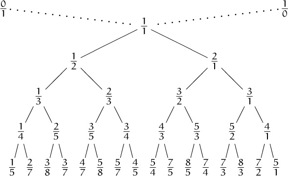
Each fraction is ![]() , where
, where ![]() is the nearest ancestor above and to the left, and
is the nearest ancestor above and to the left, and ![]() is the nearest ancestor above and to the right. (An “ancestor” is a fraction that’s reachable by following the branches upward.) Many patterns can be observed in this tree.
is the nearest ancestor above and to the right. (An “ancestor” is a fraction that’s reachable by following the branches upward.) Many patterns can be observed in this tree.
Why does this construction work? Why, for example, does each mediant fraction (m + m′)/(n + n′) turn out to be in lowest terms when it appears in this tree? (If m, m′, n, and n′ were all odd, we’d get even/even; somehow the construction guarantees that fractions with odd numerators and denominators never appear next to each other.) And why do all possible fractions m/n occur exactly once? Why can’t a particular fraction occur twice, or not at all?
Conserve parody.
All of these questions have amazingly simple answers, based on the following fundamental fact: If m/n and m′/n′ are consecutive fractions at any stage of the construction, we have
This relation is true initially (1 · 1 – 0 · 0 = 1); and when we insert a new mediant (m + m′)/(n + n′), the new cases that need to be checked are
(m + m′)n – m(n + n′) = 1;
m′(n + n′) – (m + m′)n′ = 1.
Both of these equations are equivalent to the original condition (4.31) that they replace. Therefore (4.31) is invariant at all stages of the construction.
Furthermore, if m/n < m′/n′ and if all values are nonnegative, it’s easy to verify that
m/n < (m + m′)/(n + n′) < m′/n′ .
A mediant fraction isn’t halfway between its progenitors, but it does lie somewhere in between. Therefore the construction preserves order, and we couldn’t possibly get the same fraction in two different places.
True, but if you get a compound fracture you’d better go see a doctor.
One question still remains. Can any positive fraction a/b with a ⊥ b possibly be omitted? The answer is no, because we can confine the construction to the immediate neighborhood of a/b, and in this region the behavior is easy to analyze: Initially we have
where we put parentheses around ![]() to indicate that it’s not really present yet. Then if at some stage we have
to indicate that it’s not really present yet. Then if at some stage we have
the construction forms (m + m′)/(n + n′) and there are three cases. Either (m + m′)/(n + n′) = a/b and we win; or (m + m′)/(n + n′) < a/b and we can set m ← m + m′, n ← n + n′; or (m + m′)/(n + n′) > a/b and we can set m′ ← m + m′, n′ ← n + n′. This process cannot go on indefinitely, because the conditions
imply that
an – bm ≥ 1 and bm′ – an′ ≥ 1;
hence
(m′ + n′)(an – bm) + (m + n)(bm′ – an′) ≥ m′ + n′ + m + n;
and this is the same as a + b ≥ m′ + n′ + m + n by (4.31). Either m or n or m′ or n′ increases at each step, so we must win after at most a + b steps.
The Farey series of order N, denoted by ![]() , is the set of all reduced fractions between 0 and 1 whose denominators are N or less, arranged in increasing order. For example, if N = 6 we have
, is the set of all reduced fractions between 0 and 1 whose denominators are N or less, arranged in increasing order. For example, if N = 6 we have
We can obtain ![]() in general by starting with
in general by starting with ![]() and then inserting mediants whenever it’s possible to do so without getting a denominator that is too large. We don’t miss any fractions in this way, because we know that the Stern–Brocot construction doesn’t miss any, and because a mediant with denominator ≤ N is never formed from a fraction whose denominator is > N. (In other words,
and then inserting mediants whenever it’s possible to do so without getting a denominator that is too large. We don’t miss any fractions in this way, because we know that the Stern–Brocot construction doesn’t miss any, and because a mediant with denominator ≤ N is never formed from a fraction whose denominator is > N. (In other words, ![]() defines a subtree of the Stern–Brocot tree, obtained by pruning off unwanted branches.) It follows that m′n – mn′ = 1 whenever m/n and m′/n′ are consecutive elements of a Farey series.
defines a subtree of the Stern–Brocot tree, obtained by pruning off unwanted branches.) It follows that m′n – mn′ = 1 whenever m/n and m′/n′ are consecutive elements of a Farey series.
This method of construction reveals that ![]() can be obtained in a simple way from
can be obtained in a simple way from ![]() : We simply insert the fraction (m + m′)/N between consecutive fractions m/n, m′/n′ of
: We simply insert the fraction (m + m′)/N between consecutive fractions m/n, m′/n′ of ![]() whose denominators sum to N. For example, it’s easy to obtain
whose denominators sum to N. For example, it’s easy to obtain ![]() from the elements of
from the elements of ![]() , by inserting
, by inserting ![]() according to the stated rule:
according to the stated rule:
When N is prime, N – 1 new fractions will appear; but otherwise we’ll have fewer than N – 1, because this process generates only numerators that are relatively prime to N.
Long ago in (4.5) we proved—in different words—that whenever m ⊥ n and 0 < m ≤ n we can find integers a and b such that
(Actually we said m′m + n′n = gcd(m, n), but we can write 1 for gcd(m, n), a for m′, and b for –n′.) The Farey series gives us another proof of (4.32), because we can let b/a be the fraction that precedes m/n in ![]() n. Thus (4.5) is just (4.31) again. For example, one solution to 3a – 7b = 1 is a = 5, b = 2, since
n. Thus (4.5) is just (4.31) again. For example, one solution to 3a – 7b = 1 is a = 5, b = 2, since ![]() precedes
precedes ![]() in
in ![]() 7. This construction implies that we can always find a solution to (4.32) with 0 ≤ b < a ≤ n, if 0 < m ≤ n. Similarly, if 0 ≤ n < m and m ⊥ n, we can solve (4.32) with 0 < a ≤ b ≤ m by letting a/b be the fraction that follows n/m in
7. This construction implies that we can always find a solution to (4.32) with 0 ≤ b < a ≤ n, if 0 < m ≤ n. Similarly, if 0 ≤ n < m and m ⊥ n, we can solve (4.32) with 0 < a ≤ b ≤ m by letting a/b be the fraction that follows n/m in ![]() .
.
Sequences of three consecutive terms in a Farey series have an amazing property that is proved in exercise 61. But we had better not discuss the Farey series any further, because the entire Stern–Brocot tree turns out to be even more interesting.
Farey ’nough.
We can, in fact, regard the Stern–Brocot tree as a number system for representing rational numbers, because each positive, reduced fraction occurs exactly once. Let’s use the letters L and R to stand for going down to the left or right branch as we proceed from the root of the tree to a particular fraction; then a string of L’s and R’s uniquely identifies a place in the tree. For example, LRRL means that we go left from ![]() down to
down to ![]() , then right to
, then right to ![]() , then right to
, then right to ![]() , then left to
, then left to ![]() . We can consider LRRL to be a representation of
. We can consider LRRL to be a representation of ![]() . Every positive fraction gets represented in this way as a unique string of L’s and R’s.
. Every positive fraction gets represented in this way as a unique string of L’s and R’s.
Well, actually there’s a slight problem: The fraction ![]() corresponds to the empty string, and we need a notation for that. Let’s agree to call it I, because that looks something like 1 and it stands for “identity.”
corresponds to the empty string, and we need a notation for that. Let’s agree to call it I, because that looks something like 1 and it stands for “identity.”
This representation raises two natural questions: (1) Given positive integers m and n with m ⊥ n, what is the string of L’s and R’s that corresponds to m/n? (2) Given a string of L’s and R’s, what fraction corresponds to it? Question 2 seems easier, so let’s work on it first. We define
f(S) = fraction corresponding to S
when S is a string of L’s and R’s. For example, f(LRRL) = ![]() .
.
According to the construction, f(S) = (m + m′)/(n + n′) if m/n and m′/n′ are the closest fractions preceding and following f(S) in the upper levels of the tree. Initially m/n = 0/1 and m′/n′ = 1/0; then we successively replace either m/n or m′/n′ by the mediant (m + m′)/(n + n′) as we move right or left in the tree, respectively.
How can we capture this behavior in mathematical formulas that are easy to deal with? A bit of experimentation suggests that the best way is to maintain a 2 × 2 matrix
that holds the four quantities involved in the ancestral fractions m/n and m′/n′ enclosing f(S). We could put the m’s on top and the n’s on the bottom, fractionwise; but this upside-down arrangement works out more nicely because we have ![]() when the process starts, and
when the process starts, and ![]() is traditionally called the identity matrix I.
is traditionally called the identity matrix I.
A step to the left replaces n′ by n + n′ and m′ by m + m′; hence
(This is a special case of the general rule
for multiplying 2 × 2 matrices.) Similarly it turns out that
If you’re clueless about matrices, don’t panic; this book uses them only here.
Therefore if we define L and R as 2 × 2 matrices,
we get the simple formula M(S) = S, by induction on the length of S. Isn’t that nice? (The letters L and R serve dual roles, as matrices and as letters in the string representation.) For example,
the ancestral fractions that enclose LRRL = ![]() are
are ![]() and
and ![]() . And this construction gives us the answer to Question 2:
. And this construction gives us the answer to Question 2:
How about Question 1? That’s easy, now that we understand the fundamental connection between tree nodes and 2 × 2 matrices. Given a pair of positive integers m and n, with m ⊥ n, we can find the position of m/n in the Stern–Brocot tree by “binary search” as follows:
S := I;
while m/n ≠ f(S) do
if m/n < f(S) then (output(L); S := SL)
else (output(R); S := SR).
This outputs the desired string of L’s and R’s.
There’s also another way to do the same job, by changing m and n instead of maintaining the state S. If S is any 2 × 2 matrix, we have
f(RS) = f(S) + 1
because RS is like S but with the top row added to the bottom row. (Let’s look at it in slow motion:
hence f(S) = (m + m′)/(n + n′) and f(RS) = ((m + n) + (m′ + n′)) /(n + n′).) If we carry out the binary search algorithm on a fraction m/n with m > n, the first output will be R; hence the subsequent behavior of the algorithm will have f(S) exactly 1 greater than if we had begun with (m – n)/n instead of m/n. A similar property holds for L, and we have
This means that we can transform the binary search algorithm to the following matrix-free procedure:
while m ≠ n do
if m < n then (output(L); n := n – m)
else (output(R); m := m – n) .
For example, given m/n = 5/7, we have successively
m = 5 5 3 1 1
n = 7 2 2 2 1
output L R R L
in the simplified algorithm.
Irrational numbers don’t appear in the Stern–Brocot tree, but all the rational numbers that are “close” to them do. For example, if we try the binary search algorithm with the number e = 2.71828 . . . , instead of with a fraction m/n, we’ll get an infinite string of L’s and R’s that begins
RRLRRLRLLLLRLRRRRRRLRLLLLLLLLRLR . . . .
We can consider this infinite string to be the representation of e in the Stern–Brocot number system, just as we can represent e as an infinite decimal 2.718281828459. . . or as an infinite binary fraction (10.101101111110 . . . )2. Incidentally, it turns out that e’s representation has a regular pattern in the Stern–Brocot system:
Hermann Minkowski illustrated this remarkable binary representation at the International Congress of Mathematicians in Heidelberg, 1904.
e = RL0RLR2LRL4RLR6LRL8RLR10LRL12RL . . . ;
this is equivalent to a special case of something that Euler [105] discovered when he was 24 years old.
From this representation we can deduce that the fractions
are the simplest rational upper and lower approximations to e. For if m/n does not appear in this list, then some fraction in this list whose numerator is ≤ m and whose denominator is ≤ n lies between m/n and e. For example, ![]() is not as simple an approximation as
is not as simple an approximation as ![]() , which appears in the list and is closer to e. We can see this because the Stern–Brocot tree not only includes all rationals, it includes them in order, and because all fractions with small numerator and denominator appear above all less simple ones. Thus,
, which appears in the list and is closer to e. We can see this because the Stern–Brocot tree not only includes all rationals, it includes them in order, and because all fractions with small numerator and denominator appear above all less simple ones. Thus, ![]() is less than
is less than ![]() , which is less than e = RRLRRLR . . . . Excellent approximations can be found in this way. For example,
, which is less than e = RRLRRLR . . . . Excellent approximations can be found in this way. For example, ![]() ; we obtained this fraction from the first 16 letters of e’s Stern–Brocot representation, and the accuracy is about what we would get with 16 bits of e’s binary representation.
; we obtained this fraction from the first 16 letters of e’s Stern–Brocot representation, and the accuracy is about what we would get with 16 bits of e’s binary representation.
We can find the infinite representation of an irrational number α by a simple modification of the matrix-free binary search procedure:
if α < 1 then (output(L); α := α/(1 – α))
else (output(R); α := α – 1).
(These steps are to be repeated infinitely many times, or until we get tired.) If α is rational, the infinite representation obtained in this way is the same as before but with RL∞ appended at the right of α’s (finite) representation. For example, if α = 1, we get RLLL . . . , corresponding to the infinite sequence of fractions ![]() , which approach 1 in the limit. This situation is exactly analogous to ordinary binary notation, if we think of L as 0 and R as 1: Just as every real number x in [0 . . 1) has an infinite binary representation (.b1b2b3 . . . )2 not ending with all 1’s, every real number α in [0.. ∞) has an infinite Stern–Brocot representation B1B2B3 . . . not ending with all R’s. Thus we have a one-to-one order-preserving correspondence between [0 . . 1) and [0 .. ∞) if we let 0 ↔ L and 1 ↔ R.
, which approach 1 in the limit. This situation is exactly analogous to ordinary binary notation, if we think of L as 0 and R as 1: Just as every real number x in [0 . . 1) has an infinite binary representation (.b1b2b3 . . . )2 not ending with all 1’s, every real number α in [0.. ∞) has an infinite Stern–Brocot representation B1B2B3 . . . not ending with all R’s. Thus we have a one-to-one order-preserving correspondence between [0 . . 1) and [0 .. ∞) if we let 0 ↔ L and 1 ↔ R.
There’s an intimate relationship between Euclid’s algorithm and the Stern–Brocot representations of rationals. Given α = m/n, we get ![]() m/n
m/n![]() R’s, then
R’s, then ![]() n/(m mod n)
n/(m mod n)![]() L’s, then
L’s, then ![]() (m mod n)/(n mod (m mod n))
(m mod n)/(n mod (m mod n))![]() R’s, and so on. These numbers m mod n, n mod (m mod n), . . . are just the values examined in Euclid’s algorithm. (A little fudging is needed at the end to make sure that there aren’t infinitely many R’s.) We will explore this relationship further in Chapter 6.
R’s, and so on. These numbers m mod n, n mod (m mod n), . . . are just the values examined in Euclid’s algorithm. (A little fudging is needed at the end to make sure that there aren’t infinitely many R’s.) We will explore this relationship further in Chapter 6.
4.6 ‘MOD’: The Congruence Relation
Modular arithmetic is one of the main tools provided by number theory. We got a glimpse of it in Chapter 3 when we used the binary operation ‘mod’, usually as one operation amidst others in an expression. In this chapter we will use ‘mod’ also with entire equations, for which a slightly different notation is more convenient:
“Numerorum congruentiam hoc signo,≡, in posterum denotabimus, modulum ubi opus erit in clausulis adiungentes, –16 ≡ 9 (mod. 5), –7 ≡ 15 (mod. 11).”
—C. F. Gauss [142]
For example, 9 ≡ –16 (mod 5), because 9 mod 5 = 4 = (–16) mod 5. The formula ‘a ≡ b (mod m)’ can be read “a is congruent to b modulo m.” The definition makes sense when a, b, and m are arbitrary real numbers, but we almost always use it with integers only.
Since x mod m differs from x by a multiple of m, we can understand congruences in another way:
For if a mod m = b mod m, then the definition of ‘mod’ in (3.21) tells us that a – b = a mod m + km – (b mod m + lm) = (k – l)m for some integers k and l. Conversely if a – b = km, then a = b if m = 0; otherwise
| a mod m = a – |
= b + km – |
| = b – |
The characterization of ≡ in (4.36) is often easier to apply than (4.35). For example, we have 8 ≡ 23 (mod 5) because 8 – 23 = –15 is a multiple of 5; we don’t have to compute both 8 mod 5 and 23 mod 5.
The congruence sign ‘ ≡ ’ looks conveniently like ‘ = ’, because congruences are almost like equations. For example, congruence is an equivalence relation; that is, it satisfies the reflexive law ‘a ≡ a’, the symmetric law ‘a ≡ b ⇒ b ≡ a’, and the transitive law ‘a ≡ b ≡ c ⇒ a ≡ c’. All these properties are easy to prove, because any relation ‘≡’ that satisfies ‘a ≡ b ⇔ f(a) = f(b)’ for some function f is an equivalence relation. (In our case, f(x) = x mod m.) Moreover, we can add and subtract congruent elements without losing congruence:
“I feel fine today modulo a slight headache.”
—The Hacker’s Dictionary [337]
a ≡ b and c ≡ d ![]() a + c ≡ b + d (mod m);
a + c ≡ b + d (mod m);
a ≡ b and c ≡ d ![]() a – c ≡ b – d (mod m).
a – c ≡ b – d (mod m).
For if a – b and c – d are both multiples of m, so are (a + c) – (b + d) = (a – b) + (c – d) and (a – c) – (b – d) = (a – b) – (c – d). Incidentally, it isn’t necessary to write ‘(mod m)’ once for every appearance of ‘ ≡ ’; if the modulus is constant, we need to name it only once in order to establish the context. This is one of the great conveniences of congruence notation.
Multiplication works too, provided that we are dealing with integers:
a ≡ b and c ≡ d ![]() ac ≡ bd (mod m),
ac ≡ bd (mod m),
integers b, c.
Proof: ac – bd = (a – b)c + b(c – d). Repeated application of this multiplication property now allows us to take powers:
a ≡ b ![]() an ≡ bn (mod m), integers a, b;
an ≡ bn (mod m), integers a, b;
integer n ≥ 0.
For example, since 2 ≡ –1 (mod 3), we have 2n ≡ (–1)n (mod 3); this means that 2n – 1 is a multiple of 3 if and only if n is even.
Thus, most of the algebraic operations that we customarily do with equations can also be done with congruences. Most, but not all. The operation of division is conspicuously absent. If ad ≡ bd (mod m), we can’t always conclude that a ≡ b. For example, 3·2 ≡ 5·2 (mod 4), but 3 ≢ 5.
We can salvage the cancellation property for congruences, however, in the common case that d and m are relatively prime:

For example, it’s legit to conclude from 15 ≡ 35 (mod m) that 3 ≡ 7 (mod m), unless the modulus m is a multiple of 5.
To prove this property, we use the extended gcd law (4.5) again, finding d′ and m′ such that d′d + m′m = 1. Then if ad ≡ bd we can multiply both sides of the congruence by d′, obtaining ad′d ≡ bd′d. Since d′d ≡ 1, we have ad′d ≡ a and bd′d ≡ b; hence a ≡ b. This proof shows that the number d′ acts almost like 1/d when congruences are considered (mod m); therefore we call it the “inverse of d modulo m.”
Another way to apply division to congruences is to divide the modulus as well as the other numbers:
This law holds for all real a, b, d, and m, because it depends only on the distributive law (a mod m)d = ad mod md: We have a mod m = b mod m ⇔ (a mod m)d = (b mod m)d ⇔ ad mod md = bd mod md. Thus, for example, from 3 · 2 ≡ 5 · 2 (mod 4) we conclude that 3 ≡ 5 (mod 2).
We can combine (4.37) and (4.38) to get a general law that changes the modulus as little as possible:
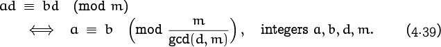
For we can multiply ad ≡ bd by d′, where d′d + m′m = gcd(d, m); this gives the congruence a · gcd(d, m) ≡ b · gcd(d, m) (mod m), which can be divided by gcd(d, m).
Let’s look a bit further into this idea of changing the modulus. If we know that a ≡ b (mod 100), then we also must have a ≡ b (mod 10), or modulo any divisor of 100. It’s stronger to say that a – b is a multiple of 100 than to say that it’s a multiple of 10. In general,
because any multiple of md is a multiple of m.
Conversely, if we know that a ≡ b with respect to two small moduli, can we conclude that a ≡ b with respect to a larger one? Yes; the rule is
Modulitos?

For example, if we know that a ≡ b modulo 12 and 18, we can safely conclude that a ≡ b (mod 36). The reason is that if a – b is a common multiple of m and n, it is a multiple of lcm(m, n). This follows from the principle of unique factorization.
The special case m ⊥ n of this law is extremely important, because lcm(m, n) = mn when m and n are relatively prime. Therefore we will state it explicitly:

For example, a ≡ b (mod 100) if and only if a ≡ b (mod 25) and a ≡ b (mod 4). Saying this another way, if we know x mod 25 and x mod 4, then we have enough facts to determine x mod 100. This is a special case of the Chinese Remainder Theorem (see exercise 30), so called because it was discovered by Sun Ts![]() in China, about A.D. 350.
in China, about A.D. 350.
The moduli m and n in (4.42) can be further decomposed into relatively prime factors until every distinct prime has been isolated. Therefore
a ≡ b (mod m) ![]() a ≡ b (mod pmp) for all p,
a ≡ b (mod pmp) for all p,
if the prime factorization (4.11) of m is Πppmp. Congruences modulo powers of primes are the building blocks for all congruences modulo integers.
4.7 Independent Residues
One of the important applications of congruences is a residue number system, in which an integer x is represented as a sequence of residues (or remainders) with respect to moduli that are prime to each other:
Res(x) = (x mod m1, . . . , x mod mr), if mj ⊥ mk for 1 ≤ j < k ≤ r.
Knowing x mod m1, . . . , x mod mr doesn’t tell us everything about x. But it does allow us to determine x mod m, where m is the product m1 . . . mr. In practical applications we’ll often know that x lies in a certain range; then we’ll know everything about x if we know x mod m and if m is large enough.
For example, let’s look at a small case of a residue number system that has only two moduli, 3 and 5:
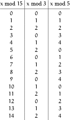
Each ordered pair (x mod 3, x mod 5) is different, because x mod 3 = y mod 3 and x mod 5 = y mod 5 if and only if x mod 15 = y mod 15.
We can perform addition, subtraction, and multiplication on the two components independently, because of the rules of congruences. For example, if we want to multiply 7 = (1, 2) by 13 = (1, 3) modulo 15, we calculate 1·1 mod 3 = 1 and 2·3 mod 5 = 1. The answer is (1, 1) = 1; hence 7·13 mod 15 must equal 1. Sure enough, it does.
This independence principle is useful in computer applications, because different components can be worked on separately (for example, by different computers). If each modulus mk is a distinct prime pk, chosen to be slightly less than 231, then a computer whose basic arithmetic operations handle integers in the range [–231 . . 231) can easily compute sums, differences, and products modulo pk. A set of r such primes makes it possible to add, subtract, and multiply “multiple-precision numbers” of up to almost 31r bits, and the residue system makes it possible to do this faster than if such large numbers were added, subtracted, or multiplied in other ways.
For example, the Mersenne prime 231 – 1 works well.
We can even do division, in appropriate circumstances. For example, suppose we want to compute the exact value of a large determinant of integers. The result will be an integer D, and bounds on |D| can be given based on the size of its entries. But the only fast ways known for calculating determinants require division, and this leads to fractions (and loss of accuracy, if we resort to binary approximations). The remedy is to evaluate D mod pk = Dk, for various large primes pk. We can safely divide modulo pk unless the divisor happens to be a multiple of pk. That’s very unlikely, but if it does happen we can choose another prime. Finally, knowing Dk for sufficiently many primes, we’ll have enough information to determine D.
But we haven’t explained how to get from a given sequence of residues (x mod m1, . . . , x mod mr) back to x mod m. We’ve shown that this conversion can be done in principle, but the calculations might be so formidable that they might rule out the idea in practice. Fortunately, there is a reasonably simple way to do the job, and we can illustrate it in the situation (x mod 3, x mod 5) shown in our little table. The key idea is to solve the problem in the two cases (1, 0) and (0, 1); for if (1, 0) = a and (0, 1) = b, then (x, y) = (ax + by) mod 15, since congruences can be multiplied and added.
In our case a = 10 and b = 6, by inspection of the table; but how could we find a and b when the moduli are huge? In other words, if m ⊥ n, what is a good way to find numbers a and b such that the equations
a mod m = 1, a mod n = 0, b mod m = 0, b mod n = 1
all hold? Once again, (4.5) comes to the rescue: With Euclid’s algorithm, we can find m′ and n′ such that
m′m + n′n = 1.
Therefore we can take a = n′n and b = m′m, reducing them both mod mn if desired.
Further tricks are needed in order to minimize the calculations when the moduli are large; the details are beyond the scope of this book, but they can be found in [208, page 274]. Conversion from residues to the corresponding original numbers is feasible, but it is sufficiently slow that we save total time only if a sequence of operations can all be done in the residue number system before converting back.
Let’s firm up these congruence ideas by trying to solve a little problem: How many solutions are there to the congruence
if we consider two solutions x and x′ to be the same when x ≡ x′?
According to the general principles explained earlier, we should consider first the case that m is a prime power, pk, where k > 0. Then the congruence x2 ≡ 1 can be written
(x – 1)(x + 1) ≡ 0 (mod pk) ,
so p must divide either x – 1 or x + 1, or both. But p can’t divide both x – 1 and x + 1 unless p = 2; we’ll leave that case for later. If p > 2, then pk(x – 1)(x + 1) ⇔ pk(x – 1) or pk(x + 1); so there are exactly two solutions, x ≡ +1 and x ≡ –1.
The case p = 2 is a little different. If 2k(x – 1)(x + 1) then either x – 1 or x + 1 is divisible by 2 but not by 4, so the other one must be divisible by 2k–1. This means that we have four solutions when k ≥ 3, namely x ≡ ±1 and x ≡ 2k–1 ± 1. (For example, when pk = 8 the four solutions are x ≡ 1, 3, 5, 7 (mod 8); it’s often useful to know that the square of any odd integer has the form 8n + 1.)
Now x2 ≡ 1 (mod m) if and only if x2 ≡ 1 (mod pmp) for all primes p with mp > 0 in the complete factorization of m. Each prime is independent of the others, and there are exactly two possibilities for x mod pmp except when p = 2. Therefore if m has exactly r different prime divisors, the total number of solutions to x2 ≡ 1 is 2r, except for a correction when m is even. The exact number in general is
All primes are odd except 2, which is the oddest of all.
For example, there are four “square roots of unity modulo 12,” namely 1, 5, 7, and 11. When m = 15 the four are those whose residues mod 3 and mod 5 are ±1, namely (1, 1), (1, 4), (2, 1), and (2, 4) in the residue number system. These solutions are 1, 4, 11, and 14 in the ordinary (decimal) number system.
4.8 Additional Applications
There’s some unfinished business left over from Chapter 3: We wish to prove that the m numbers
consist of precisely d copies of the m/d numbers
0, d, 2d, ..., m – d
in some order, where d = gcd(m, n). For example, when m = 12 and n = 8 we have d = 4, and the numbers are 0, 8, 4, 0, 8, 4, 0, 8, 4, 0, 8, 4.
The first part of the proof—to show that we get d copies of the first m/d values—is now trivial. We have
Mathematicians love to say that things are trivial.
jn ≡ kn (mod m) ![]() j(n/d) ≡ k(n/d) (mod m/d)
j(n/d) ≡ k(n/d) (mod m/d)
by (4.38); hence we get d copies of the values that occur when 0 ≤ k < m/d.
Now we must show that those m/d numbers are {0, d, 2d, . . . , m – d} in some order. Let’s write m = m′d and n = n′d. Then kn mod m = d(kn′ mod m′), by the distributive law (3.23); so the values that occur when 0 ≤ k < m′ are d times the numbers
0 mod m′, n′ mod m′, 2n′ mod m′, . . . , (m′ – 1)n′ mod m′ .
But we know that m′ ⊥ n′ by (4.27); we’ve divided out their gcd. Therefore we need only consider the case d = 1, namely the case that m and n are relatively prime.
So let’s assume that m ⊥ n. In this case it’s easy to see that the numbers (4.45) are just {0, 1, . . . , m – 1} in some order, by using the “pigeonhole principle.” This principle states that if m pigeons are put into m pigeonholes, there is an empty hole if and only if there’s a hole with more than one pigeon. (Dirichlet’s box principle, proved in exercise 3.8, is similar.) We know that the numbers (4.45) are distinct, because
jn ≡ kn (mod m) ![]() j ≡ k (mod m)
j ≡ k (mod m)
when m ⊥ n; this is (4.37). Therefore the m different numbers must fill all the pigeonholes 0, 1, . . . , m – 1. Therefore the unfinished business of Chapter 3 is finished.
The proof is complete, but we can prove even more if we use a direct method instead of relying on the indirect pigeonhole argument. If m ⊥ n and if a value j ∈ [0 . . m) is given, we can explicitly compute k ∈ [0 . . m) such that kn mod m = j by solving the congruence
kn ≡ j (mod m)
for k. We simply multiply both sides by n′, where m′m + n′n = 1, to get
k ≡ jn′ (mod m);
hence k = jn′ mod m.
We can use the facts just proved to establish an important result discovered by Pierre de Fermat in 1640. Fermat was a great mathematician who contributed to the discovery of calculus and many other parts of mathematics. He left notebooks containing dozens of theorems stated without proof, and each of those theorems has subsequently been verified—including one that became the most famous of all, because it baffled the world’s best mathematicians for 350 years. The famous one, called “Fermat’s Last Theorem,” states that
for all positive integers a, b, c, and n, when n > 2. (Of course there are lots of solutions to the equations a + b = c and a2 + b2 = c2.) Andrew Wiles has apparently settled the question at long last; his intricate, epoch-making proof of (4.46) appears in Annals of Mathematics (2) 141 (1995), 443–551.
NEWS FLASH
Euler [115] conjectured that a4 + b4 + c4 ≠ d4, but Noam Elkies [92] found infinitely many solutions in August, 1987.
Now Roger Frye has done an exhaustive computer search, proving (after about 110 hours on a Connection Machine) that the only solution with d < 1000000 is: 958004 + 2175194 + 4145604 = 4224814.
Fermat’s theorem of 1640 is much easier to verify. It’s now called Fermat’s Little Theorem (or just Fermat’s theorem, for short), and it states that
Proof: As usual, we assume that p denotes a prime. We know that the p – 1 numbers n mod p, 2n mod p, . . . , (p – 1)n mod p are the numbers 1, 2, . . . , p – 1 in some order. Therefore if we multiply them together we get
| n · (2n) · . . . · ((p – 1)n) | |
| ≡ (n mod p) · (2n mod p) · . . . · ((p – 1)n mod p) | |
| ≡ (p – 1)!, | |
where the congruence is modulo p. This means that
(p – 1)! np–1 ≡ (p – 1)! (mod p),
and we can cancel the (p – 1)! since it’s not divisible by p. QED.
An alternative form of Fermat’s theorem is sometimes more convenient:
This congruence holds for all integers n. The proof is easy: If n ⊥ p we simply multiply (4.47) by n. If not, pn, so np ≡ 0 ≡ n.
In the same year that he discovered (4.47), Fermat wrote a letter to Mersenne, saying he suspected that the number
fn = 22n + 1
would turn out to be prime for all n ≥ 0. He knew that the first five cases gave primes:
“. . . laquelle proposition, si elle est vraie, est de très grand usage.”
—P. de Fermat [121]
21+1 = 3; 22+1 = 5; 24+1 = 17; 28+1 = 257; 216+1 = 65537;
but he couldn’t see how to prove that the next case, 232 + 1 = 4294967297, would be prime.
It’s interesting to note that Fermat could have proved that 232 + 1 is not prime, using his own recently discovered theorem, if he had taken time to perform a few dozen multiplications: We can set n = 3 in (4.47), deducing that
3232 ≡ 1 (mod 232 + 1), if 232 + 1 is prime.
And it’s possible to test this relation by hand, beginning with 3 and squaring 32 times, keeping only the remainders mod 232 + 1. First we have 32 = 9, then 322 = 81, then 323 = 6561, and so on until we reach
If this is Fermat’s Little Theorem, the other one was last but not least.
3232 ≡ 3029026160 (mod 232 + 1) .
The result isn’t 1, so 232 + 1 isn’t prime. This method of disproof gives us no clue about what the factors might be, but it does prove that factors exist. (They are 641 and 6700417, first found by Euler in 1732 [102].)
If 3232 had turned out to be 1, modulo 232 + 1, the calculation wouldn’t have proved that 232 + 1 is prime; it just wouldn’t have disproved it. But exercise 47 discusses a converse to Fermat’s theorem by which we can prove that large prime numbers are prime, without doing an enormous amount of laborious arithmetic.
We proved Fermat’s theorem by cancelling (p – 1)! from both sides of a congruence. It turns out that (p – 1)! is always congruent to –1, modulo p; this is part of a classical result known as Wilson’s theorem:
One half of this theorem is trivial: If n > 1 is not prime, it has a prime divisor p that appears as a factor of (n – 1)!, so (n – 1)! cannot be congruent to –1. (If (n–1)! were congruent to –1 modulo n, it would also be congruent to –1 modulo p, but it isn’t.)
The other half of Wilson’s theorem states that (p – 1)! ≡ –1 (mod p). We can prove this half by pairing up numbers with their inverses mod p. If n ⊥ p, we know that there exists n′ such that
n′n ≡ 1 (mod p);
here n′ is the inverse of n, and n is also the inverse of n′. Any two inverses of n must be congruent to each other, since nn′ ≡ nn″ implies n′ ≡ n″.
If p is prime, is p′ prime prime?
Now suppose we pair up each number between 1 and p–1 with its inverse. Since the product of a number and its inverse is congruent to 1, the product of all the numbers in all pairs of inverses is also congruent to 1; so it seems that (p – 1)! is congruent to 1. Let’s check, say for p = 5. We get 4! = 24; but this is congruent to 4, not 1, modulo 5. Oops—what went wrong? Let’s take a closer look at the inverses:
1′ = 1, 2′ = 3, 3′ = 2, 4′ = 4.
Ah so; 2 and 3 pair up but 1 and 4 don’t—they’re their own inverses.
To resurrect our analysis we must determine which numbers are their own inverses. If x is its own inverse, then x2 ≡ 1 (mod p); and we have already proved that this congruence has exactly two roots when p > 2. (If p = 2 it’s obvious that (p – 1)! ≡ –1, so we needn’t worry about that case.) The roots are 1 and p – 1, and the other numbers (between 1 and p – 1) pair up; hence
(p – 1)! ≡ 1 · (p – 1) ≡ –1,
as desired.
Unfortunately, we can’t compute factorials efficiently, so Wilson’s theorem is of no use as a practical test for primality. It’s just a theorem.
4.9 PHI and MU
How many of the integers {0, 1, . . . , m – 1} are relatively prime to m? This is an important quantity called φ(m), the “totient” of m (so named by J. J. Sylvester [347], a British mathematician who liked to invent new words). We have φ(1) = 1, φ(p) = p – 1, and φ(m) < m – 1 for all composite numbers m.
The φ function is called Euler’s totient function, because Euler was the first person to study it. Euler discovered, for example, that Fermat’s theorem (4.47) can be generalized to nonprime moduli in the following way:
“Si fuerit N ad x numerus primus et n numerus partium ad N primarum, tum potestas xn unitate minuta semper per numerum N erit divisibilis.”
—L. Euler [111]
(Exercise 32 asks for a proof of Euler’s theorem.)
If m is a prime power pk, it’s easy to compute φ(m), because we have ![]() . The multiples of p in {0, 1, . . . , pk – 1} are {0, p, 2p, . . . , pk – p}; hence there are pk–1 of them, and φ(pk) counts what is left:
. The multiples of p in {0, 1, . . . , pk – 1} are {0, p, 2p, . . . , pk – p}; hence there are pk–1 of them, and φ(pk) counts what is left:
φ(pk) = pk – pk –1 .
Notice that this formula properly gives φ(p) = p – 1 when k = 1.
If m > 1 is not a prime power, we can write m = m1m2 where m1 ⊥ m2. Then the numbers 0 ≤ n < m can be represented in a residue number system as (n mod m1, n mod m2). We have
n ⊥ m ![]() n mod m1 ⊥ m1 and n mod m2 ⊥ m2
n mod m1 ⊥ m1 and n mod m2 ⊥ m2
by (4.30) and (4.4). Hence, n mod m is “good” if and only if n mod m1 and n mod m2 are both “good,” if we consider relative primality to be a virtue. The total number of good values modulo m can now be computed, recursively: It is φ(m1)φ(m2), because there are φ(m1) good ways to choose the first component n mod m1 and φ(m2) good ways to choose the second component n mod m2 in the residue representation.
For example, φ(12) = φ(4)φ(3) = 2·2 = 4, because n is prime to 12 if and only if n mod 4 = (1 or 3) and n mod 3 = (1 or 2). The four values prime to 12 are (1, 1), (1, 2), (3, 1), (3, 2) in the residue number system; they are 1, 5, 7, 11 in ordinary decimal notation. Euler’s theorem states that n4 ≡ 1 (mod 12) whenever n ⊥ 12.
“Si sint A et B numeri inter se primi et numerus partium ad A primarum sit = a, numerus vero partium ad B primarum sit = b, tum numerus partium ad productum AB primarum erit = ab.”
—L. Euler [111]
A function f(m) of positive integers is called multiplicative if f(1) = 1 and
We have just proved that φ(m) is multiplicative. We’ve also seen another instance of a multiplicative function earlier in this chapter: The number of incongruent solutions to x2 ≡ 1 (mod m) is multiplicative. Still another example is f(m) = mα for any power α.
A multiplicative function is defined completely by its values at prime powers, because we can decompose any positive integer m into its prime-power factors, which are relatively prime to each other. The general formula
holds if and only if f is multiplicative.
In particular, this formula gives us the value of Euler’s totient function for general m:

For example, ![]() .
.
Now let’s look at an application of the φ function to the study of rational numbers mod 1. We say that the fraction m/n is basic if 0 ≤ m < n. Therefore φ(n) is the number of reduced basic fractions with denominator n; and the Farey series ![]() contains all the reduced basic fractions with denominator n or less, as well as the non-basic fraction
contains all the reduced basic fractions with denominator n or less, as well as the non-basic fraction ![]() .
.
The set of all basic fractions with denominator 12, before reduction to lowest terms, is
Reduction yields
and we can group these fractions by their denominators:
What can we make of this? Well, every divisor d of 12 occurs as a denominator, together with all φ(d) of its numerators. The only denominators that occur are divisors of 12. Thus
φ(1) + φ(2) + φ(3) + φ(4) + φ(6) + φ(12) = 12.
A similar thing will obviously happen if we begin with the unreduced fractions ![]() for any m, hence
for any m, hence
We said near the beginning of this chapter that problems in number theory often require sums over the divisors of a number. Well, (4.54) is one such sum, so our claim is vindicated. (We will see other examples.)
Now here’s a curious fact: If f is any function such that the sum
is multiplicative, then f itself is multiplicative. (This result, together with (4.54) and the fact that g(m) = m is obviously multiplicative, gives another reason why φ(m) is multiplicative.) We can prove this curious fact by induction on m: The basis is easy because f(1) = g(1) = 1. Let m > 1, and assume that f(m1m2) = f(m1)f(m2) whenever m1 ⊥ m2 and m1m2 < m. If m = m1m2 and m1 ⊥ m2, we have
and d1 ⊥ d2 since all divisors of m1 are relatively prime to all divisors of m2. By the induction hypothesis, f(d1d2) = f(d1)f(d2) except possibly when d1 = m1 and d2 = m2; hence we obtain
But this equals g(m1m2) = g(m1)g(m2), so f(m1m2) = f(m1)f(m2).
Conversely, if f(m) is multiplicative, the corresponding sum-over-divisors function g(m) = ∑dm f(d) is always multiplicative. In fact, exercise 33 shows that even more is true. Hence the curious fact and its converse are both facts.
The Möbius function μ(m), named after the nineteenth-century mathematician August Möbius who also had a famous band, can be defined for all integers m ≥ 1 by the equation
This equation is actually a recurrence, since the left-hand side is a sum consisting of μ(m) and certain values of μ(d) with d < m. For example, if we plug in m = 1, 2, . . . , 12 successively we can compute the first twelve values:

Richard Dedekind [77] and Joseph Liouville [251] noticed the following important “inversion principle” in 1857:

According to this principle, the μ function gives us a new way to understand any function f(m) for which we know ∑dm f(d).
Now is a good time to try warmup exercise 11.
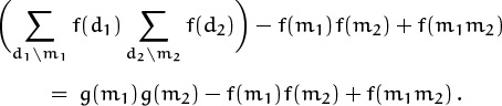
The proof of (4.56) uses two tricks (4.7) and (4.9) that we described near the beginning of this chapter: If g(m) = ∑dm f(d) then

The other half of (4.56) is proved similarly (see exercise 12).
Relation (4.56) gives us a useful property of the Möbius function, and we have tabulated the first twelve values; but what is the value of μ(m) when m is large? How can we solve the recurrence (4.55)? Well, the function g(m) = [m = 1] is obviously multiplicative—after all, it’s zero except when m = 1. So the Möbius function defined by (4.55) must be multiplicative, by the curious fact we proved a minute or two ago. Therefore we can figure out what μ(m) is if we compute μ(pk).
Depending on how fast you read.
When m = pk, (4.55) says that
μ(1) + μ(p) + μ(p2) + · · · + μ(pk) = 0
for all k ≥ 1, since the divisors of pk are 1, . . . , pk. It follows that
µ(p) = –1; µ(pk) = 0 for k > 1.
Therefore by (4.52), we have the general formula

That’s μ.
If we regard (4.54) as a recurrence for the function φ(m), we can solve that recurrence by applying the Dedekind-Liouville rule (4.56). We get

For example,
| φ(12) | = µ(1)·12 + µ(2)·6 + µ(3)·4 + µ(4)·3 + µ(6)·2 + µ(12)·1 |
| = 12 – 6 – 4 + 0 + 2 + 0 = 4. |
If m is divisible by r different primes, say {p1, . . . , pr}, the sum (4.58) has only 2r nonzero terms, because the μ function is often zero. Thus we can see that (4.58) checks with formula (4.53), which reads
if we multiply out the r factors (1 – 1/pj), we get precisely the 2r nonzero terms of (4.58). The advantage of the Möbius function is that it applies in many situations besides this one.
For example, let’s try to figure out how many fractions are in the Farey series ![]() . This is the number of reduced fractions in [0 . . 1] whose denominators do not exceed n, so it is 1 greater than Φ(n) where we define
. This is the number of reduced fractions in [0 . . 1] whose denominators do not exceed n, so it is 1 greater than Φ(n) where we define
(We must add 1 to Φ(n) because of the final fraction ![]() .) The sum in (4.59) looks difficult, but we can determine Φ(x) indirectly by observing that
.) The sum in (4.59) looks difficult, but we can determine Φ(x) indirectly by observing that

for all real x ≥ 0. Why does this identity hold? Well, it’s a bit awesome yet not really beyond our ken. There are ![]() basic fractions m/n with 0 ≤ m < n ≤ x, counting both reduced and unreduced fractions; that gives us the right-hand side. The number of such fractions with gcd(m, n) = d is Φ(x/d), because such fractions are m′/n′ with 0 ≤ m′ < n′ ≤ x/d after replacing m by m′d and n by n′d. So the left-hand side counts the same fractions in a different way, and the identity must be true.
basic fractions m/n with 0 ≤ m < n ≤ x, counting both reduced and unreduced fractions; that gives us the right-hand side. The number of such fractions with gcd(m, n) = d is Φ(x/d), because such fractions are m′/n′ with 0 ≤ m′ < n′ ≤ x/d after replacing m by m′d and n by n′d. So the left-hand side counts the same fractions in a different way, and the identity must be true.
Let’s look more closely at the situation, so that equations (4.59) and (4.60) become clearer. The definition of Φ(x) implies that Φ(x) = Φ (![]() x
x![]() ); but it turns out to be convenient to define Φ(x) for arbitrary real values, not just for integers. At integer values we have the table
); but it turns out to be convenient to define Φ(x) for arbitrary real values, not just for integers. At integer values we have the table
(This extension to real values is a useful trick for many recurrences that arise in the analysis of algorithms.)
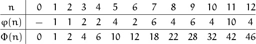
and we can check (4.60) when x = 12:
Φ(12) + Φ(6) + Φ(4) + Φ(3) + Φ(2) + Φ(2) + 6·Φ(1)
= 46 + 12 + 6 + 4 + 2 + 2 + 6 = 78 = ![]() · 12 · 13.
· 12 · 13.
Amazing.
Identity (4.60) can be regarded as an implicit recurrence for Φ(x); for example, we’ve just seen that we could have used it to calculate Φ(12) from certain values of Φ(m) with m < 12. And we can solve such recurrences by using another beautiful property of the Möbius function:
In fact, Möbius [273] invented his function because of (4.61), not (4.56).
This inversion law holds for all functions f such that ∑k,d≥1|f(x/kd)| < ∞; we can prove it as follows. Suppose g(x) = ∑d≥1 f(x/d). Then
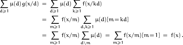
The proof in the other direction is essentially the same.
So now we can solve the recurrence (4.60) for Φ(x):

This is always a finite sum. For example,
| Φ(12) | = |
| – 1·2 + 0 + 0 + 1·2 – 1·2 + 0) | |
| = 78 – 21 – 10 – 3 + 3 – 1 + 1 – 1 = 46. |
In Chapter 9 we’ll see how to use (4.62) to get a good approximation to Φ(x); in fact, we’ll prove a result due to Mertens in 1874 [270],
Φ(x) = ![]() x2 + O(x log x) .
x2 + O(x log x) .
Therefore the function Φ(x) grows “smoothly”; it averages out the erratic behavior of φ(k).
In keeping with the tradition established last chapter, let’s conclude this chapter with a problem that illustrates much of what we’ve just seen and that also points ahead to the next chapter. Suppose we have beads of n different colors; our goal is to count how many different ways there are to string them into circular necklaces of length m. We can try to “name and conquer” this problem by calling the number of possible necklaces N(m, n).
For example, with two colors of beads R and B, we can make necklaces of length 4 in N(4, 2) = 6 different ways:
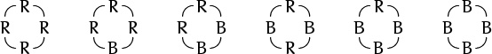
All other ways are equivalent to one of these, because rotations of a necklace do not change it. However, reflections are considered to be different; in the case m = 6, for example,
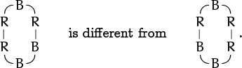
The problem of counting these configurations was first solved by P. A. MacMahon in 1892 [264].
There’s no obvious recurrence for N(m, n), but we can count the necklaces by breaking them each into linear strings in m ways and considering the resulting fragments. For example, when m = 4 and n = 2 we get
RRRR RRRR RRRR RRRR
RRBR RRRB BRRR RBRR
RBBR RRBB BRRB BBRR .
RBRB BRBR RBRB BRBR
RBBB BRBB BBRB BBBR
BBBB BBBB BBBB BBBB
Each of the nm possible patterns appears at least once in this array of mN(m, n) strings, and some patterns appear more than once. How many times does a pattern a0 . . . am–1 appear? That’s easy: It’s the number of cyclic shifts ak . . . am–1 a0 . . . ak–1 that produce the same pattern as the original a0 . . . am–1. For example, BRBR occurs twice, because the four ways to cut the necklace formed from BRBR produce four cyclic shifts (BRBR, RBRB, BRBR, RBRB); two of these coincide with BRBR itself. This argument shows that
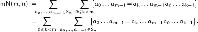
Here Sn is a set of n different colors.
Let’s see how many patterns satisfy a0 . . . am–1 = ak . . . am–1 a0 . . . ak–1, when k is given. For example, if m = 12 and k = 8, we want to count the number of solutions to
a0a1a2a3a4a5a6a7a8a9a10a11 = a8a9a10a11a0a1a2a3a4a5a6a7 .
This means a0 = a8 = a4; a1 = a9 = a5; a2 = a10 = a6; and a3 = a11 = a7. So the values of a0, a1, a2, and a3 can be chosen in n4 ways, and the remaining a’s depend on them. Does this look familiar? In general, the solution to
aj = a(j+k) mod m, for 0 ≤ j < m
makes us equate aj with a(j+kl) mod m for l = 1, 2, . . . ; and we know that the multiples of k modulo m are {0, d, 2d, . . . , m – d}, where d = gcd(k, m). Therefore the general solution is to choose a0, . . . , ad–1 independently and then to set aj = aj–d for d ≤ j < m. There are nd solutions.
We have just proved that
This sum can be simplified, since it includes only terms nd where dm. Substituting d = gcd(k, m) yields
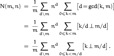
(We are allowed to replace k/d by k because k must be a multiple of d.) Finally, we have ∑0≤k<m/d[k ⊥ m/d] = φ(m/d) by definition, so we obtain MacMahon’s formula:

When m = 4 and n = 2, for example, the number of necklaces is ![]() , just as we suspected.
, just as we suspected.
It’s not immediately obvious that the value N(m, n) defined by MacMahon’s sum is an integer! Let’s try to prove directly that
without using the clue that this is related to necklaces. In the special case that m is prime, this congruence reduces to np + (p – 1)n ≡ 0 (mod p); that is, it reduces to np ≡ n. We’ve seen in (4.48) that this congruence is an alternative form of Fermat’s theorem. Therefore (4.64) holds when m = p; we can regard it as a generalization of Fermat’s theorem to the case when the modulus is not prime. (Euler’s generalization (4.50) is different.)
We’ve proved (4.64) for all prime moduli, so let’s look at the smallest case left, m = 4. We must prove that
n4 + n2 + 2n ≡ 0 (mod 4).
The proof is easy if we consider even and odd cases separately. If n is even, all three terms on the left are congruent to 0 modulo 4, so their sum is too. If n is odd, n4 and n2 are each congruent to 1, and 2n is congruent to 2; hence the left side is congruent to 1 + 1 + 2 and thus to 0 modulo 4, and we’re done.
Next, let’s be a bit daring and try m = 12. This value of m ought to be interesting because it has lots of factors, including the square of a prime, yet it is fairly small. (Also there’s a good chance we’ll be able to generalize a proof for 12 to a proof for general m.) The congruence we must prove is
Now what? By (4.42) this congruence holds if and only if it also holds modulo 3 and modulo 4. So let’s prove that it holds modulo 3. Our congruence (4.64) holds for primes, so we have n3 + 2n ≡ 0 (mod 3). Careful scrutiny reveals that we can use this fact to group terms of the larger sum:
n12 + n6 + 2n4 + 2n3 + 2n2 + 4n
= (n12 + 2n4) + (n6 + 2n2) + 2(n3 + 2n)
≡ 0 + 0 + 2·0 ≡ 0 (mod 3) .
So it works modulo 3.
We’re half done. To prove congruence modulo 4 we use the same trick. We’ve proved that n4 + n2 + 2n ≡ 0 (mod 4), so we use this pattern to group:
n12 + n6 + 2n4 + 2n3 + 2n2 + 4n
= (n12 + n6 + 2n3) + 2(n4 + n2 + 2n)
≡ 0 + 2·0 ≡ 0 (mod 4) .
QED: Quite Easily Done.
QED for the case m = 12.
So far we’ve proved our congruence for prime m, for m = 4, and for m = 12. Now let’s try to prove it for prime powers. For concreteness we may suppose that m = p3 for some prime p. Then the left side of (4.64) is
np3 + φ(p)np2 + φ(p2)np + φ(p3)n
= np3 + (p – 1)np2 + (p2 – p)np + (p3 – p2)n
= (np3 – np2) + p(np2 – np) + p2(np – n) + p3n.
We can show that this is congruent to 0 modulo p3 if we can prove that np3– np2 is divisible by p3, that np2– np is divisible by p2, and that np – n is divisible by p, because the whole thing will then be divisible by p3. By the alternative form of Fermat’s theorem we have np ≡ n (mod p), so p divides np – n; hence there is an integer q such that
np = n + pq.
Now we raise both sides to the pth power, expand the right side according to the binomial theorem (which we’ll meet in Chapter 5), and regroup, giving
np2 = (n + pq)p = np + (pq)1np–1 ![]() + (pq)2np–2
+ (pq)2np–2 ![]() + · · ·
+ · · ·
= np + p2Q
for some other integer Q. We’re able to pull out a factor of p2 here because ![]() in the second term, and because a factor of (pq)2 appears in all the terms that follow. So we find that p2 divides np2 – np.
in the second term, and because a factor of (pq)2 appears in all the terms that follow. So we find that p2 divides np2 – np.
Again we raise both sides to the pth power, expand, and regroup, to get
np3 = (np + p2Q)p
= np2 + (p2Q)1np(p–1) ![]() + (p2Q)2np(p–2)
+ (p2Q)2np(p–2) ![]() + · · ·
+ · · ·
= np2 + p3Q
for yet another integer Q. So p3 divides np3 – np2. This finishes the proof for m = p3, because we’ve shown that p3 divides the left-hand side of (4.64).
Moreover we can prove by induction that
npk = npk –1 + pk![]()
for some final integer ![]() (final because we’re running out of fonts); hence
(final because we’re running out of fonts); hence
Thus the left side of (4.64), which is
(npk– npk–1) + p(npk–1 – npk–2) + · · · + pk–1(np – n) + pkn,
is divisible by pk and so is congruent to 0 modulo pk.
We’re almost there. Now that we’ve proved (4.64) for prime powers, all that remains is to prove it when m = m1m2, where m1 ⊥ m2, assuming that the congruence is true for m1 and m2. Our examination of the case m = 12, which factored into instances of m = 3 and m = 4, encourages us to think that this approach will work.
We know that the φ function is multiplicative, so we can write
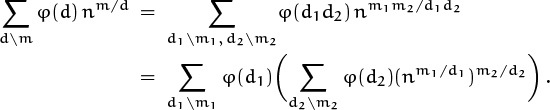
But the inner sum is congruent to 0 modulo m2, because we’ve assumed that (4.64) holds for m2; so the entire sum is congruent to 0 modulo m2. By a symmetric argument, we find that the entire sum is congruent to 0 modulo m1 as well. Thus by (4.42) it’s congruent to 0 modulo m. QED.
Exercises
Warmups
1. What is the smallest positive integer that has exactly k divisors, for 1 ≤ k ≤ 6?
2. Prove that gcd(m, n)·lcm(m, n) = m·n, and use this identity to express lcm(m, n) in terms of lcm(n mod m, m), when n mod m ≠ 0. Hint: Use (4.12), (4.14), and (4.15).
3. Let π(x) be the number of primes not exceeding x. Prove or disprove:
π(x) – π(x – 1) = [x is prime] .
4. What would happen if the Stern–Brocot construction started with the five fractions ![]() instead of with
instead of with ![]() ?
?
5. Find simple formulas for Lk and Rk, when L and R are the 2 × 2 matrices of (4.33).
6. What does ‘a ≡ b (mod 0)’ mean?
7. Ten people numbered 1 to 10 are lined up in a circle as in the Josephus problem, and every mth person is executed. (The value of m may be much larger than 10.) Prove that the first three people to go cannot be 10, k, and k + 1 (in this order), for any k.
8. The residue number system (x mod 3, x mod 5) considered in the text has the curious property that 13 corresponds to (1, 3), which looks almost the same. Explain how to find all instances of such a coincidence, without calculating all fifteen pairs of residues. In other words, find all relevant solutions to the congruences
Hint: Use the facts that 10u + 6v ≡ u (mod 3) and 10u + 6v ≡ v (mod 5).
9. Show that (377 – 1)/2 is odd and composite. Hint: What is 377 mod 4?
10. Compute φ(999).
11. Find a function σ(n) with the property that
(This is analogous to the Möbius function; see (4.56).)
12. Simplify the formula ∑dm ∑kd μ(k) g(d/k).
13. A positive integer n is called squarefree if it is not divisible by m2 for any m > 1. Find a necessary and sufficient condition that n is squarefree,
a. in terms of the prime-exponent representation (4.11) of n;
b. in terms of μ(n).
Basics
14. Prove or disprove:
a. gcd(km, kn) = k gcd(m, n);
b. lcm(km, kn) = k lcm(m, n).
15. Does every prime occur as a factor of some Euclid number en?
16. What is the sum of the reciprocals of the first n Euclid numbers?
17. Let fn be the “Fermat number” 22n + 1. Prove that fm ⊥ fn if m < n.
18. Show that if 2n + 1 is prime then n is a power of 2.
19. Prove the following identities when n is a positive integer:
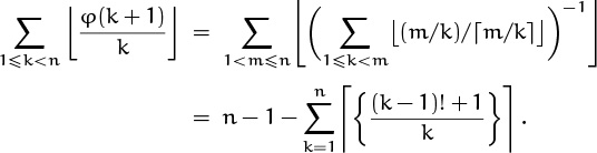
Hint: This is a trick question and the answer is pretty easy.
20. For every positive integer n there’s a prime p such that n < p ≤ 2n. (This is essentially “Bertrand’s postulate,” which Joseph Bertrand verified for n < 3000000 in 1845 and Chebyshev proved for all n in 1850.) Use Bertrand’s postulate to prove that there’s a constant b ≈ 1.25 such that the numbers
![]() 2b
2b![]() ,
, ![]() 22b
22b![]() ,
, ![]() 222b
222b ![]() , . . .
, . . .
are all prime.
21. Let Pn be the nth prime number. Find a constant K such that
![]() (10n2 K) mod 10n
(10n2 K) mod 10n ![]() = Pn .
= Pn .
22. The number 1111111111111111111 is prime. Prove that, in any radix b, (11 . . . 1)b can be prime only if the number of 1’s is prime.
Is this a test for strabismus?
23. State a recurrence for ρ(k), the ruler function in the text’s discussion of ![]() 2(n!). Show that there’s a connection between ρ(k) and the disk that’s moved at step k when an n-disk Tower of Hanoi is being transferred in 2n – 1 moves, for 1 ≤ k ≤ 2n – 1.
2(n!). Show that there’s a connection between ρ(k) and the disk that’s moved at step k when an n-disk Tower of Hanoi is being transferred in 2n – 1 moves, for 1 ≤ k ≤ 2n – 1.
24. Express ![]() p(n!) in terms of νp(n), the sum of the digits in the radix p representation of n, thereby generalizing (4.24).
p(n!) in terms of νp(n), the sum of the digits in the radix p representation of n, thereby generalizing (4.24).
Look, ma, sideways addition.
25. We say that m exactly divides n, written m\n, if mn and m ⊥ n/m. For example, in the text’s discussion of factorial factors, p![]() p(n!)\n!. Prove or disprove the following:
p(n!)\n!. Prove or disprove the following:
a. k\n and m\n ⇔ km\n, if k ⊥ m.
b. For all m, n > 0, either gcd(m, n)\m or gcd(m, n)\n.
26. Consider the sequence ![]() of all nonnegative reduced fractions m/n such that mn ≤ N. For example,
of all nonnegative reduced fractions m/n such that mn ≤ N. For example,
Is it true that m′n – mn′ = 1 whenever m/n immediately precedes m′/n′ in ![]() ?
?
27. Give a simple rule for comparing rational numbers based on their representations as L’s and R’s in the Stern–Brocot number system.
28. The Stern–Brocot representation of π is
π = R3L7R15LR292LRLR2LR3LR14L2R . . . ;
use it to find all the simplest rational approximations to π whose denominators are less than 50. Is ![]() one of them?
one of them?
29. The text describes a correspondence between binary real numbers x = (.b1b2b3 . . . )2 in [0 . . 1) and Stern–Brocot real numbers α = B1B2B3 . . . in [0 .. ∞). If x corresponds to α and x ≠ 0, what number corresponds to 1 – x?
30. Prove the following statement (the Chinese Remainder Theorem): Let m1, . . . , mr be positive integers with mj ⊥ mk for 1 ≤ j < k ≤ r; let m = m1 . . . mr; and let a1, . . . , ar, A be integers. Then there is exactly one integer a such that
31. A number in decimal notation is divisible by 3 if and only if the sum of its digits is divisible by 3. Prove this well-known rule, and generalize it.
32. Prove Euler’s theorem (4.50) by generalizing the proof of (4.47).
Why is “Euler” pronounced “Oiler” when “Euclid” is “Yooklid”?
33. Show that if f(m) and g(m) are multiplicative functions, then so is h(m) = ∑dm f(d) g(m/d).
34. Prove that (4.56) is a special case of (4.61).
Homework exercises
35. Let I(m, n) be a function that satisfies the relation
I(m, n)m + I(n, m)n = gcd(m, n),
when m and n are nonnegative integers with m ≠ n. Thus, I(m, n) = m′ and I(n, m) = n′ in (4.5); the value of I(m, n) is an inverse of m with respect to n. Find a recurrence that defines I(m, n).
36. Consider the set ![]() | integer m, n}. The number
| integer m, n}. The number ![]() is called a unit if m2 – 10n2 = ±1, since it has an inverse (that is, since
is called a unit if m2 – 10n2 = ±1, since it has an inverse (that is, since ![]() . For example,
. For example, ![]() is a unit, and so is
is a unit, and so is ![]() . Pairs of cancelling units can be inserted into any factorization, so we ignore them. Nonunit numbers of
. Pairs of cancelling units can be inserted into any factorization, so we ignore them. Nonunit numbers of ![]() are called prime if they cannot be written as a product of two nonunits. Show that 2, 3, and
are called prime if they cannot be written as a product of two nonunits. Show that 2, 3, and ![]() are primes of
are primes of ![]() . Hint: If
. Hint: If ![]() then 4 = (k2 – 10l2)(m2 – 10n2). Furthermore, the square of any integer mod 10 is 0, 1, 4, 5, 6, or 9.
then 4 = (k2 – 10l2)(m2 – 10n2). Furthermore, the square of any integer mod 10 is 0, 1, 4, 5, 6, or 9.
37. Prove (4.17). Hint: Show that ![]() , and consider
, and consider ![]() .
.
38. Prove that if a ⊥ b and a > b > 0 then
gcd(am – bm, an – bn) = agcd(m,n) – bgcd(m,n), 0 ≤ m < n.
(All variables are integers.) Hint: Use Euclid’s algorithm.
39. Let S(m) be the smallest positive integer n for which there exists an increasing sequence of integers
m = a1 < a2 < · · · < at = n
such that a1a2 . . . at is a perfect square. (If m is a perfect square, we can let t = 1 and n = m.) For example, S(2) = 6 because the best such sequence is a1 = 2, a2 = 3, a3 = 6. We have
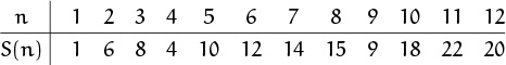
Prove that S(m) ≠ S(m′) whenever 0 < m < m′.
40. If the radix p representation of n is (am . . . a1a0)p, prove that
n!/pεp(n!) ≡ (–1)εp(n!) am! . . . a1! a0! (mod p) .
(The left side is simply n! with all p factors removed. When n = p this reduces to Wilson’s theorem.)
Wilson’s theorem: “Martha, that boy is a menace.”
41.
a. Show that if p mod 4 = 3, there is no integer n such that p divides n2 + 1. Hint: Use Fermat’s theorem.
b. But show that if p mod 4 = 1, there is such an integer. Hint: Write (p – 1)! as ![]() and think about Wilson’s theorem.
and think about Wilson’s theorem.
42. Consider two fractions m/n and m′/n′ in lowest terms. Prove that when the sum m/n + m′/n′ is reduced to lowest terms, the denominator will be nn′ if and only if n ⊥ n′. (In other words, (mn′ + m′n)/nn′ will already be in lowest terms if and only if n and n′ have no common factor.)
43. There are 2k nodes at level k of the Stern–Brocot tree, corresponding to the matrices Lk, Lk–1 R, . . . , Rk. Show that this sequence can be obtained by starting with Lk and then multiplying successively by
for 1 ≤ n < 2k, where ρ(n) is the ruler function.
44. Prove that a baseball player whose batting average is .316 must have batted at least 19 times. (If he has m hits in n times at bat, then m/n ∈ [0.3155 . . 0.3165).)
45. The number 9376 has the peculiar self-reproducing property that
93762 = 87909376.
Radio announcer:
“. . . pitcher Mark LeChiffre hits a two-run single! Mark, who was batting .080, gets his second hit of the year.”
Anything wrong?
How many 4-digit numbers x satisfy the equation x2 mod 10000 = x?
How many n-digit numbers x satisfy the equation x2 mod 10n = x?
46.
a. Prove that if nj ≡ 1 and nk ≡ 1 (mod m), then ngcd(j,k) ≡ 1.
b. Show that 2n ≢ 1 (mod n), if n > 1. Hint: Consider the least prime factor of n.
47. Show that if nm–1 ≡ 1 (mod m) and if n(m–1)/p ≢ 1 (mod m) for all primes such that p(m – 1), then m is prime. Hint: Show that if this condition holds, the numbers nk mod m are distinct, for 1 ≤ k < m.
48. Generalize Wilson’s theorem (4.49) by ascertaining the value of the expression (Π1≤n<m, n⊥m n) mod m, when m > 1.
49. Let R(N) be the number of pairs of integers (m, n) such that 1 ≤ m ≤ N, 1 ≤ n ≤ N, and m ⊥ n.
a. Express R(N) in terms of the Φ function.
b. Prove that R(N) = ∑d≥1 ![]() N/d
N/d![]() 2μ(d).
2μ(d).
50. Let m be a positive integer and let
ω = e2πi/m = cos(2π/m) + i sin(2π/m) .
We say that ω is an mth root of unity, since ωm = e2πi = 1. In fact, each of the m complex numbers ω0, ω1, . . . , ωm–1 is an mth root of unity, because (ωk)m = e2πki = 1; therefore z – ωk is a factor of the polynomial zm – 1, for 0 ≤ k < m. Since these factors are distinct, the complete factorization of zm – 1 over the complex numbers must be
What are the roots of disunity?
a. Let ![]() . (This polynomial of degree φ(m) is called the cyclotomic polynomial of order m.) Prove that
. (This polynomial of degree φ(m) is called the cyclotomic polynomial of order m.) Prove that
b. Prove that ![]() .
.
Exam problems
51. Prove Fermat’s theorem (4.48) by expanding (1 + 1 + · · · + 1)p via the multinomial theorem.
52. Let n and x be positive integers such that x has no divisors ≤ n (except 1), and let p be a prime number. Prove that at least ![]() n/p
n/p![]() of the numbers {x – 1, x2 – 1, . . . , xn –1 – 1} are multiples of p.
of the numbers {x – 1, x2 – 1, . . . , xn –1 – 1} are multiples of p.
53. Find all positive integers n such that n ![]() (n – 1)!/(n + 1)
(n – 1)!/(n + 1)![]() .
.
54. Determine the value of 1000! mod 10250 by hand calculation.
55. Let Pn be the product of the first n factorials, ![]() . Prove that
. Prove that ![]() is an integer, for all positive integers n.
is an integer, for all positive integers n.
56. Show that
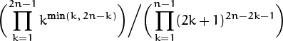
is a power of 2.
57. Let S(m, n) be the set of all integers k such that
m mod k + n mod k ≥ k.
For example, S(7, 9) = {2, 4, 5, 8, 10, 11, 12, 13, 14, 15, 16}. Prove that
Hint: Prove first that ![]() . Then consider
. Then consider ![]() (m + n)/d
(m + n)/d![]() –
– ![]() m/d
m/d![]() –
– ![]() n/d
n/d![]() .
.
58. Let f(m) = ∑dm d. Find a necessary and sufficient condition that f(m) is a power of 2.
Bonus problems
59. Prove that if x1, . . . , xn are positive integers with 1/x1 + · · · + 1/xn = 1, then max(x1, . . . , xn) < en. Hint: Prove the following stronger result by induction: “If 1/x1 + · · · + 1/xn + 1/α = 1, where x1, . . . , xn are positive integers and α is a rational number ≥ max(x1, . . . , xn), then α+1 ≤ en+1 and x1 . . . xn(α + 1) ≤ e1 . . . en en+1.” (The proof is nontrivial.)
60. Prove that there’s a constant P such that (4.18) gives only primes. You may use the following (highly nontrivial) fact: There is a prime between p and p + pθ, for all sufficiently large p, if ![]() .
.
61. Prove that if m/n, m′/n′, and m″/n″ are consecutive elements of ![]() , then
, then
m″ = ![]() (n + N)/n′
(n + N)/n′![]() m′ – m,
m′ – m,
n″ = ![]() (n + N)/n′
(n + N)/n′![]() n′ – n.
n′ – n.
(This recurrence allows us to compute the elements of ![]() in order, starting with
in order, starting with ![]() and
and ![]() .)
.)
62. What binary number corresponds to e, in the binary ↔ Stern–Brocot correspondence? (Express your answer as an infinite sum; you need not evaluate it in closed form.)
63. Using only the methods of this chapter, show that if Fermat’s Last Theorem (4.46) were false, the least n for which it fails would have to be prime. (You may assume that (4.46) holds when n = 4.) Furthermore, if ap + bp = cp is the smallest counterexample, show that
for some integer m. Thus c ≥ mp/2 must be really huge. Hint: Let x = a + b, and note that gcd (x, (ap + (x – a)p)/x) = gcd(x, pap–1).
64. The Peirce sequence ![]() of order N is an infinite string of fractions separated by ‘<’ or ‘=’ signs, containing all the nonnegative fractions m/n with m ≥ 0 and n ≤ N (including fractions that are not reduced). It is defined recursively by starting with
of order N is an infinite string of fractions separated by ‘<’ or ‘=’ signs, containing all the nonnegative fractions m/n with m ≥ 0 and n ≤ N (including fractions that are not reduced). It is defined recursively by starting with
For N ≥ 1, we form ![]() N+1 by inserting two symbols just before the kNth symbol of
N+1 by inserting two symbols just before the kNth symbol of ![]() N, for all k > 0. The two inserted symbols are
N, for all k > 0. The two inserted symbols are
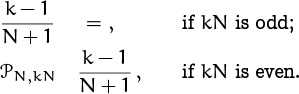
Here ![]() N, j denotes the jth symbol of
N, j denotes the jth symbol of ![]() N, which will be either ‘<’ or ‘=’ when j is even; it will be a fraction when j is odd. For example,
N, which will be either ‘<’ or ‘=’ when j is even; it will be a fraction when j is odd. For example,
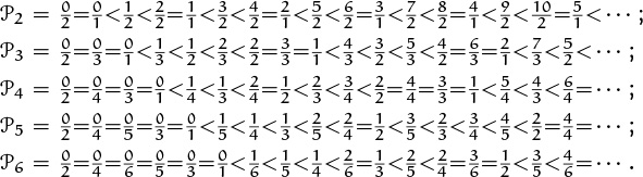
(Equal elements occur in a slightly peculiar order.) Prove that the ‘<’ and ‘=’ signs defined by the rules above correctly describe the relations between adjacent fractions in the Peirce sequence.
Research problems
65. Are the Euclid numbers en all squarefree?
66. Are the Mersenne numbers 2p – 1 all squarefree?
67. Prove or disprove that max1≤j<k≤n ak/gcd(aj, ak) ≥ n, for all sequences of integers 0 < a1 < · · · < an.
68. Is there a constant Q such that ![]() Q2n
Q2n![]() is prime for all n ≥ 0?
is prime for all n ≥ 0?
69. Let Pn denote the nth prime. Prove or disprove that Pn+1 – Pn = O(log Pn)2.
70. Does ![]() 3(n!) =
3(n!) = ![]() 2(n!)/2 for infinitely many n?
2(n!)/2 for infinitely many n?
71. Prove or disprove: If k ≠ 1 there exists n > 1 such that 2n ≡ k (mod n). Are there infinitely many such n?
72. Prove or disprove: For all integers a, there exist infinitely many n such that φ(n)(n + a).
73. If the Φ(n) + 1 terms of the Farey series
were fairly evenly distributed, we would expect ![]() n(k) ≈ k/Φ(n). Therefore the sum
n(k) ≈ k/Φ(n). Therefore the sum ![]() measures the “deviation of
measures the “deviation of ![]() n from uniformity.” Is it true that D(n) = O(n1/2+
n from uniformity.” Is it true that D(n) = O(n1/2+![]() ) for all
) for all ![]() > 0?
> 0?
74. Approximately how many distinct values are there in the set {0! mod p, 1! mod p, . . . , (p – 1)! mod p}, as p → ∞?