
9. Asymptotics
Exact answers are great when we can find them; there’s something very satisfying about complete knowledge. But there’s also a time when approximations are in order. If we run into a sum or a recurrence whose solution doesn’t have a closed form (as far as we can tell), we still would like to know something about the answer; we don’t have to insist on all or nothing. And even if we do have a closed form, our knowledge might be imperfect, since we might not know how to compare it with other closed forms.
Uh oh . . . here comes that A-word.
For example, there is (apparently) no closed form for the sum

But it is nice to know that
we say that the sum is “asymptotic to” ![]() . It’s even nicer to have more detailed information, like
. It’s even nicer to have more detailed information, like
which gives us a “relative error of order 1/n2.” But even this isn’t enough to tell us how big Sn is, compared with other quantities. Which is larger, Sn or the Fibonacci number F4n? Answer: We have S2 = 22 > F8 = 21 when n = 2; but F4n is eventually larger, because F4n ∼ ϕ4n/ ![]() and ϕ4 ≈ 6.8541, while
and ϕ4 ≈ 6.8541, while

Our goal in this chapter is to learn how to understand and to derive results like this without great pain.
Other words like ‘symptom’ and ‘ptomaine’ also come from this root.
The word asymptotic stems from a Greek root meaning “not falling together.” When ancient Greek mathematicians studied conic sections, they considered hyperbolas like the graph of ![]() ,
,
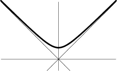
which has the lines y = x and y = –x as “asymptotes.” The curve approaches but never quite touches these asymptotes, when x → ∞. Nowadays we use “asymptotic” in a broader sense to mean any approximate value that gets closer and closer to the truth, when some parameter approaches a limiting value. For us, asymptotics means “almost falling together.”
Some asymptotic formulas are very difficult to derive, well beyond the scope of this book. We will content ourselves with an introduction to the subject; we hope to acquire a suitable foundation on which further techniques can be built. We will be particularly interested in understanding the definitions of ‘∼’ and ‘O’ and similar symbols, and we’ll study basic ways to manipulate asymptotic quantities.
9.1 A Hierarchy
Functions of n that occur in practice usually have different “asymptotic rates of growth”; one of them will approach infinity faster than another. We formalize this by saying that
This relation is transitive: If f(n) ≺ g(n) and g(n) ≺ h(n) then f(n) ≺ h(n). We also may write g(n) ≻ f(n) if f(n) ≺ g(n). This notation was introduced in 1871 by Paul du Bois-Reymond [85].
All functions great and small.
For example, n ≺ n2; informally we say that n grows more slowly than n2. In fact,
when α and β are arbitrary real numbers.
There are, of course, many functions of n besides powers of n. We can use the ≺ relation to rank lots of functions into an asymptotic pecking order that includes entries like this:
1 ≺ log log n ≺ log n ≺ n![]() ≺ nc ≺ nlog n ≺ cn ≺ nn ≺ ccn .
≺ nc ≺ nlog n ≺ cn ≺ nn ≺ ccn .
(Here ![]() and c are arbitrary constants with 0 <
and c are arbitrary constants with 0 < ![]() < 1 < c.)
< 1 < c.)
All functions listed here, except 1, go to infinity as n goes to infinity. Thus when we try to place a new function in this hierarchy, we’re not trying to determine whether it becomes infinite but rather how fast.
It helps to cultivate an expansive attitude when we’re doing asymptotic analysis: We should THINK BIG, when imagining a variable that approaches infinity. For example, the hierarchy says that log n ≺ n0.0001; this might seem wrong if we limit our horizons to teeny-tiny numbers like one googol, n = 10100. For in that case, log n = 100, while n0.0001 is only 100.01 ≈ 1.0233. But if we go up to a googolplex, n = 1010100, then log n = 10100 pales in comparison with n0.0001 = 101096.
Even if ![]() is extremely small (smaller than, say, 1/1010100), the value of log n will be much smaller than the value of n
is extremely small (smaller than, say, 1/1010100), the value of log n will be much smaller than the value of n![]() , if n is large enough. For if we set n = 10102k, where k is so large that
, if n is large enough. For if we set n = 10102k, where k is so large that ![]() ≥ 10–k, we have log n = 102k but n
≥ 10–k, we have log n = 102k but n![]() ≥ 1010k. The ratio (log n)/n
≥ 1010k. The ratio (log n)/n![]() therefore approaches zero as n → ∞.
therefore approaches zero as n → ∞.
A loerarchy?
The hierarchy shown above deals with functions that go to infinity. Often, however, we’re interested in functions that go to zero, so it’s useful to have a similar hierarchy for those functions. We get one by taking reciprocals, because when f(n) and g(n) are never zero we have
Thus, for example, the following functions (except 1) all go to zero:
Let’s look at a few other functions to see where they fit in. The number π(n) of primes less than or equal to n is known to be approximately n/ln n. Since 1/n![]() ≺ 1/ln n ≺ 1, multiplying by n tells us that
≺ 1/ln n ≺ 1, multiplying by n tells us that
n1–![]() ≺ π(n) ≺ n.
≺ π(n) ≺ n.
We can in fact generalize (9.4) by noticing, for example, that

Here ‘(α1, α2, α3) < (β1, β2, β3)’ means lexicographic order (dictionary order); in other words, either α1 < β1, or α1 = β1 and α2 < β2, or α1 = β1 and α2 = β2 and α3 < β3.
How about the function ![]() ; where does it live in the hierarchy? We can answer questions like this by using the rule
; where does it live in the hierarchy? We can answer questions like this by using the rule
which follows in two steps from definition (9.3) by taking logarithms. Consequently
1 ≺ f(n) ≺ g(n) = e|f (n)| ≺ e|g(n)| .
And since ![]() , we have
, we have ![]() .
.
When two functions f(n) and g(n) have the same rate of growth, we write ‘f(n) ≍ g(n)’. The official definition is:

This holds, for example, if f(n) = cos n + arctan n and g(n) is a nonzero constant. We will prove shortly that it holds whenever f(n) and g(n) are polynomials of the same degree. There’s also a stronger relation, defined by the rule
In this case we say that “f(n) is asymptotic to g(n).”
G. H. Hardy [179] introduced an interesting and important concept called the class of logarithmico-exponential functions, defined recursively as the smallest family ![]() of functions satisfying the following properties:
of functions satisfying the following properties:
• The constant function f(n) = α is in ![]() , for all real α.
, for all real α.
• The identity function f(n) = n is in ![]() .
.
• If f(n) and g(n) are in ![]() , so is f(n) – g(n).
, so is f(n) – g(n).
• If f(n) is in ![]() , so is ef(n).
, so is ef(n).
• If f(n) is in ![]() and is “eventually positive,” then ln f(n) is in
and is “eventually positive,” then ln f(n) is in ![]() .
.
A function f(n) is called “eventually positive” if there is an integer n0 such that f(n) > 0 whenever n ≥ n0.
We can use these rules to show, for example, that f(n) + g(n) is in ![]() whenever f(n) and g(n) are, because f(n) + g(n) = f(n) – (0 – g(n)). If f(n) and g(n) are eventually positive members of
whenever f(n) and g(n) are, because f(n) + g(n) = f(n) – (0 – g(n)). If f(n) and g(n) are eventually positive members of ![]() , their product f(n)g(n) = e ln f(n)+ln g(n) and quotient f(n)/g(n) = e ln f(n)–ln g(n) are in
, their product f(n)g(n) = e ln f(n)+ln g(n) and quotient f(n)/g(n) = e ln f(n)–ln g(n) are in ![]() ; so are functions like
; so are functions like ![]() , etc. Hardy proved that every logarithmico-exponential function is eventually positive, eventually negative, or identically zero. Therefore the product and quotient of any two
, etc. Hardy proved that every logarithmico-exponential function is eventually positive, eventually negative, or identically zero. Therefore the product and quotient of any two ![]() -functions are in
-functions are in ![]() , except that we cannot divide by a function that’s identically zero.
, except that we cannot divide by a function that’s identically zero.
Hardy’s main theorem about logarithmico-exponential functions is that they form an asymptotic hierarchy: If f(n) and g(n) are any functions in ![]() , then either f(n) ≺ g(n), or f(n) ≻ g(n), or f(n) ≍ g(n). In the last case there is, in fact, a constant α such that
, then either f(n) ≺ g(n), or f(n) ≻ g(n), or f(n) ≍ g(n). In the last case there is, in fact, a constant α such that
f(n) ∼ α g(n).
The proof of Hardy’s theorem is beyond the scope of this book; but it’s nice to know that the theorem exists, because almost every function we ever need to deal with is in ![]() . In practice, we can generally fit a given function into a given hierarchy without great difficulty.
. In practice, we can generally fit a given function into a given hierarchy without great difficulty.
9.2 O Notation
A wonderful notational convention for asymptotic analysis was introduced by Paul Bachmann in 1894 and popularized in subsequent years by Edmund Landau and others. We have seen it in formulas like
which tells us that the nth harmonic number is equal to the natural logarithm of n plus Euler’s constant, plus a quantity that is “Big Oh of 1 over n.” This last quantity isn’t specified exactly; but whatever it is, the notation claims that its absolute value is no more than a constant times 1/n.
“. . . , wenn wir durch das Zeichen O(n) eine Grosse ausdrucken, deren Ordnung in Bezug auf n die Ordnung von n nicht uberschreitet; ob sie wirklich Glieder von der Ordnung n in sich enthalt, bleibt bei dem bisherigen Schlussverfahren dahingestellt.”
—P. Bachmann [17]
The beauty of O-notation is that it suppresses unimportant detail and lets us concentrate on salient features: The quantity O(1/n) is negligibly small, if constant multiples of 1/n are unimportant.
Furthermore we get to use O right in the middle of a formula. If we want to express (9.10) in terms of the notations in Section 9.1, we must transpose ‘ln n + γ’ to the left side and specify a weaker result like
Hn – ln n – γ ≺ ![]()
or a stronger result like
Hn – ln n – γ ≍ ![]()
The Big Oh notation allows us to specify an appropriate amount of detail in place, without transposition.
The idea of imprecisely specified quantities can be made clearer if we consider some additional examples. We occasionally use the notation ‘±1’ to stand for something that is either +1 or –1; we don’t know (or perhaps we don’t care) which it is, yet we can manipulate it in formulas.
N. G. de Bruijn begins his book Asymptotic Methods in Analysis [74] by considering a Big Ell notation that helps us understand Big Oh. If we write L(5) for a number whose absolute value is less than 5 (but we don’t say what the number is), then we can perform certain calculations without knowing the full truth. For example, we can deduce formulas such as 1 + L(5) = L(6); L(2) + L(3) = L(5); L(2)L(3) = L(6); eL(5) = L(e5); and so on. But we cannot conclude that L(5) – L(3) = L(2), since the left side might be 4 – 0. In fact, the most we can say is L(5) – L(3) = L(8).
It’s not nonsense, but it is pointless.
Bachmann’s O-notation is similar to L-notation but it’s even less precise: O(α) stands for a number whose absolute value is at most a constant times |α|. We don’t say what the number is and we don’t even say what the constant is. Of course the notion of a “constant” is nonsense if there is nothing variable in the picture, so we use O-notation only in contexts when there’s at least one quantity (say n) whose value is varying. The formula
means in this context that there is a constant C such that
and when O (g(n)) stands in the middle of a formula it represents a function f(n) that satisfies (9.12). The values of f(n) are unknown, but we do know that they aren’t too large. Similarly, the quantity L(n) above represents an unspecified function f(n) whose values satisfy |f(n)| < |n|. The main difference between L and O is that O-notation involves an unspecified constant C; each appearance of O might involve a different C, but each C is independent of n.
For example, we know that the sum of the first n squares is
We can write
□n = O(n3)
because ![]() for all integers n. Similarly, we have the more specific formula
for all integers n. Similarly, we have the more specific formula
□n = ![]() n3 + O(n2);
n3 + O(n2);
we can also be sloppy and throw away information, saying that
□n = O(n10).
Nothing in the definition of O requires us to give a best possible bound.
I’ve got a little list—I’ve got a little list, Of annoying terms and details that might well be under ground, And that never would be missed—that never would be missed.
But wait a minute. What if the variable n isn’t an integer? What if we have a formula like S(x) = ![]() x3 +
x3 + ![]() x2 +
x2 + ![]() x, where x is a real number? Then we cannot say that S(x) = O(x3), because the ratio S(x)/x3 =
x, where x is a real number? Then we cannot say that S(x) = O(x3), because the ratio S(x)/x3 = ![]() +
+ ![]() x–1 +
x–1 + ![]() x–2 becomes unbounded when x → 0. And we cannot say that S(x) = O(x), because the ratio S(x)/x =
x–2 becomes unbounded when x → 0. And we cannot say that S(x) = O(x), because the ratio S(x)/x = ![]() x2 +
x2 + ![]() x +
x + ![]() becomes unbounded when x → ∞. So we apparently can’t use O-notation with S(x).
becomes unbounded when x → ∞. So we apparently can’t use O-notation with S(x).
The answer to this dilemma is that variables used with O are generally subject to side conditions. For example, if we stipulate that |x| ≥ 1, or that x ≥ ![]() where
where ![]() is any positive constant, or that x is an integer, then we can write S(x) = O(x3). If we stipulate that |x| ≤ 1, or that |x| ≤ c where c is any positive constant, then we can write S(x) = O(x). The O-notation is governed by its environment, by constraints on the variables involved.
is any positive constant, or that x is an integer, then we can write S(x) = O(x3). If we stipulate that |x| ≤ 1, or that |x| ≤ c where c is any positive constant, then we can write S(x) = O(x). The O-notation is governed by its environment, by constraints on the variables involved.
You are the fairest of your sex, Let me be your hero; I love you as one over x, As x approaches zero.
—Michael Stueben Positively.
These constraints are often specified by a limiting relation. For example, we might say that
This means that the O-condition is supposed to hold when n is “near” ∞; we don’t care what happens unless n is quite large. Moreover, we don’t even specify exactly what “near” means; in such cases each appearance of O implicitly asserts the existence of two constants C and n0, such that
The values of C and n0 might be different for each O, but they do not depend on n. Similarly, the notation
| f(x) = O (g(x)) | as x → 0 |
means that there exist two constants C and ![]() such that
such that
The limiting value does not have to be ∞ or 0; we can write
| ln z = z – 1 + O ((z – 1)2) | as z → 1, |
because it can be proved that | ln z – z + 1| ≤ |z – 1|2 when |z – 1| ≤ ![]() .
.
Our definition of O has gradually developed, over a few pages, from something that seemed pretty obvious to something that seems rather complex; we now have O representing an undefined function and either one or two unspecified constants, depending on the environment. This may seem complicated enough for any reasonable notation, but it’s still not the whole story! Another subtle consideration lurks in the background. Namely, we need to realize that it’s fine to write
![]() n3 +
n3 + ![]() n2 +
n2 + ![]() n = O(n3),
n = O(n3),
but we should never write this equality with the sides reversed. Otherwise we could deduce ridiculous things like n = n2 from the identities n = O(n2) and n2 = O(n2). When we work with O-notation and any other formulas that involve imprecisely specified quantities, we are dealing with one-way equalities. The right side of an equation does not give more information than the left side, and it may give less; the right is a “crudification” of the left.
“And to auoide the tediouse repetition of these woordes: is equalle to: I will sette as I doe often in woorke use, a paire of paralleles, or Gemowe lines of one lengthe, thus: ====, bicause noe .2. thynges, can be moare equalle.”
—R. Recorde [305]
From a strictly formal point of view, the notation O (g(n)) does not stand for a single function f(n), but for the set of all functions f(n) such that |f(n)| ≤ C| g(n)| for some constant C. An ordinary formula g(n) that doesn’t involve O-notation stands for the set containing a single function f(n) = g(n). If S and T are sets of functions of n, the notation S + T stands for the set of all functions of the form f(n) + g(n), where f(n) ![]() S and g(n)
S and g(n) ![]() T; other notations like S–T, ST, S/T,
T; other notations like S–T, ST, S/T, ![]() , eS, ln S are defined similarly. Then an “equation” between such sets of functions is, strictly speaking, a set inclusion; the ‘=’ sign really means ‘⊆’. These formal definitions put all of our O manipulations on firm logical ground.
, eS, ln S are defined similarly. Then an “equation” between such sets of functions is, strictly speaking, a set inclusion; the ‘=’ sign really means ‘⊆’. These formal definitions put all of our O manipulations on firm logical ground.
For example, the “equation”
![]() n3 + O(n2) = O(n3)
n3 + O(n2) = O(n3)
means that S1 ⊆ S2, where S1 is the set of all functions of the form ![]() n3 + f1(n) such that there exists a constant C1 with |f1(n)| ≤ C1|n2|, and where S2 is the set of all functions f2(n) such that there exists a constant C2 with |f2(n)| ≤ C2|n3|. We can formally prove this “equation” by taking an arbitrary element of the left-hand side and showing that it belongs to the right-hand side: Given
n3 + f1(n) such that there exists a constant C1 with |f1(n)| ≤ C1|n2|, and where S2 is the set of all functions f2(n) such that there exists a constant C2 with |f2(n)| ≤ C2|n3|. We can formally prove this “equation” by taking an arbitrary element of the left-hand side and showing that it belongs to the right-hand side: Given ![]() n3 + f1 (n) such that |f1(n)| ≤ C1|n2|, we must prove that there’s a constant C2 such that
n3 + f1 (n) such that |f1(n)| ≤ C1|n2|, we must prove that there’s a constant C2 such that ![]() n3 + f1 (n)| ≤ C2|n3|. The constant C2 =
n3 + f1 (n)| ≤ C2|n3|. The constant C2 = ![]() + C1 does the trick, since n2 ≤ |n3| for all integers n.
+ C1 does the trick, since n2 ≤ |n3| for all integers n.
If ‘=’ really means ‘⊆’, why don’t we use ‘⊆’ instead of abusing the equals sign? There are four reasons.
First, tradition. Number theorists started using the equals sign with O-notation and the practice stuck. It’s sufficiently well established by now that we cannot hope to get the mathematical community to change.
Second, tradition. Computer people are quite used to seeing equals signs abused—for years FORTRAN and BASIC programmers have been writing assignment statements like ‘N = N + 1’. One more abuse isn’t much.
Third, tradition. We often read ‘=’ as the word ‘is’. For instance we verbalize the formula Hn = O(log n) by saying “H sub n is Big Oh of log n.” And in English, this ‘is’ is one-way. We say that a bird is an animal, but we don’t say that an animal is a bird; “animal” is a crudification of “bird.”
Fourth, for our purposes it’s natural. If we limited our use of O-notation to situations where it occupies the whole right side of a formula—as in the harmonic number approximation Hn = O(log n), or as in the description of a sorting algorithm’s running time T(n) = O(n log n)—it wouldn’t matter whether we used ‘=’ or something else. But when we use O-notation in the middle of an expression, as we usually do in asymptotic calculations, our intuition is well satisfied if we think of the equals sign as an equality, and if we think of something like O(1/n) as a very small quantity.
“It is obvious that the sign = is really the wrong sign for such relations, because it suggests symmetry, and there is no such symmetry. . . . Once this warning has been given, there is, however, not much harm in using the sign =, and we shall maintain it, for no other reason than that it is customary.”
—N. G. de Bruijn [74]
So we’ll continue to use ‘=’, and we’ll continue to regard O (g(n)) as an incompletely specified function, knowing that we can always fall back on the set-theoretic definition if we must.
But we ought to mention one more technicality while we’re picking nits about definitions: If there are several variables in the environment, O-notation formally represents sets of functions of two or more variables, not just one. The domain of each function is every variable that is currently “free” to vary.
This concept can be a bit subtle, because a variable might be defined only in parts of an expression, when it’s controlled by a Σ or something similar. For example, let’s look closely at the equation

The expression k2 + O(k) on the left stands for the set of all two-variable functions of the form k2 + f(k, n) such that there exists a constant C with |f(k, n)| ≤ Ck for 0 ≤ k ≤ n. The sum of this set of functions, for 0 ≤ k ≤ n, is the set of all functions g(n) of the form

where f has the stated property. Since we have
| | |
|
| ≤ |
|
| < n2 + C(n2 + n)/2 < (C + 1)n2, | |
all such functions g(n) belong to the right-hand side of (9.16); therefore (9.16) is true.
(Now is a good time to do warmup exercises 3 and 4.)
People sometimes abuse O-notation by assuming that it gives an exact order of growth; they use it as if it specifies a lower bound as well as an upper bound. For example, an algorithm to sort n numbers might be called inefficient “because its running time is O(n2).” But a running time of O(n2) does not imply that the running time is not also O(n). There’s another notation, Big Omega, for lower bounds:
We have f(n) = Ω (g(n)) if and only if g(n) = O (f(n)) . A sorting algorithm whose running time is Ω(n2) is inefficient compared with one whose running time is O(n log n), if n is large enough.
Since Ω and Θ are uppercase Greek letters, the O in O-notation must be a capital Greek Omicron. After all, Greeks invented asymptotics.
Finally there’s Big Theta, which specifies an exact order of growth:
We have f(n) = Θ (g(n)) if and only if f(n) ≍ g(n) in the notation we saw previously, equation (9.8).
Edmund Landau [238] invented a “little oh” notation,

This is essentially the relation f(n) ≺ g(n) of (9.3). We also have
Many authors use ‘o’ in asymptotic formulas, but a more explicit ‘O’ expression is almost always preferable. For example, the average running time of a computer method called “bubblesort” depends on the asymptotic value of the sum ![]() . Elementary asymptotic methods suffice to prove the formula
. Elementary asymptotic methods suffice to prove the formula ![]() , which means that the ratio
, which means that the ratio ![]() approaches 1 as n → ∞. However, the true behavior of P(n) is best understood by considering the difference,
approaches 1 as n → ∞. However, the true behavior of P(n) is best understood by considering the difference, ![]() , not the ratio:
, not the ratio:
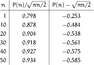
The numerical evidence in the middle column is not very compelling; it certainly is far from a dramatic proof that ![]() approaches 1 rapidly, if at all. But the right-hand column shows that P(n) is very close indeed to
approaches 1 rapidly, if at all. But the right-hand column shows that P(n) is very close indeed to ![]() . Thus we can characterize the behavior of P(n) much better if we can derive formulas of the form
. Thus we can characterize the behavior of P(n) much better if we can derive formulas of the form
or even sharper estimates like
Stronger methods of asymptotic analysis are needed to prove O-results, but the additional effort required to learn these stronger methods is amply compensated by the improved understanding that comes with O-bounds.
Moreover, many sorting algorithms have running times of the form
T(n) = A n lg n + B n + O(log n)
for some constants A and B. Analyses that stop at T(n) ∼ A n lg n don’t tell the whole story, and it turns out to be a bad strategy to choose a sorting algorithm based just on its A value. Algorithms with a good ‘A’ often achieve this at the expense of a bad ‘B’. Since n lg n grows only slightly faster than n, the algorithm that’s faster asymptotically (the one with a slightly smaller A value) might be faster only for values of n that never actually arise in practice. Thus, asymptotic methods that allow us to go past the first term and evaluate B are necessary if we are to make the right choice of method.
Also lD, the Duraflame logarithm.
Before we go on to study O, let’s talk about one more small aspect of mathematical style. Three different notations for logarithms have been used in this chapter: lg, ln, and log. We often use ‘lg’ in connection with computer methods, because binary logarithms are often relevant in such cases; and we often use ‘ln’ in purely mathematical calculations, since the formulas for natural logarithms are nice and simple. But what about ‘log’? Isn’t this the “common” base-10 logarithm that students learn in high school—the “common” logarithm that turns out to be very uncommon in mathematics and computer science? Yes; and many mathematicians confuse the issue by using ‘log’ to stand for natural logarithms or binary logarithms. There is no universal agreement here. But we can usually breathe a sigh of relief when a logarithm appears inside O-notation, because O ignores multiplicative constants. There is no difference between O(lg n), O(ln n), and O(log n), as n → ∞; similarly, there is no difference between O(lg lg n), O(ln ln n), and O(log log n). We get to choose whichever we please; and the one with ‘log’ seems friendlier because it is more pronounceable. Therefore we generally use ‘log’ in all contexts where it improves readability without introducing ambiguity.
Notice that log log log n is undefined when n ≤ 10.
9.3 O Manipulation
Like any mathematical formalism, the O-notation has rules of manipulation that free us from the grungy details of its definition. Once we prove that the rules are correct, using the definition, we can henceforth work on a higher plane and forget about actually verifying that one set of functions is contained in another. We don’t even need to calculate the constants C that are implied by each O, as long as we follow rules that guarantee the existence of such constants.
The secret of being a bore is to tell everything.
—Voltaire
For example, we can prove once and for all that
Then we can say immediately that ![]() n3+
n3+ ![]() n2+
n2+ ![]() n = O(n3)+O(n3)+O(n3) = O(n3), without the laborious calculations in the previous section.
n = O(n3)+O(n3)+O(n3) = O(n3), without the laborious calculations in the previous section.
Here are some more rules that follow easily from the definition:
Exercise 9 proves (9.22), and the proofs of the others are similar. We can always replace something of the form on the left by what’s on the right, regardless of the side conditions on the variable n.
(Note: The formula O(f(n))2 does not denote the set of all functions g(n)2 where g(n) is in O(f(n)); such functions g(n)2 cannot be negative, but the set O(f(n))2 includes negative functions. In general, when S is a set, the notation S2 stands for the set of all products s1s2 with s1 and s2 in S, not for the set of all squares s2 with s ![]() S.)
S.)
Equations (9.27) and (9.23) allow us to derive the identity O (f(n)2) = O (f(n))2. This sometimes helps avoid parentheses, since we can write
| O(log n)2 | instead of | O((log n)2). |
Both of these are preferable to ‘O(log2 n)’, which is ambiguous because some authors use it to mean ‘O(log log n)’.
Can we also write
| O(log n)–1 | instead of | O((log n)–1) ? |
No! This is an abuse of notation, since the set of functions 1/O(log n) is neither a subset nor a superset of O(1/log n). We could legitimately substitute Ω(log n)–1 for O ((log n)–1), but this would be awkward. So we’ll restrict our use of “exponents outside the O” to constant, positive integer exponents.
Power series give us some of the most useful operations of all. If the sum
converges absolutely for some complex number z = z0, then
| S(z) = O(1), | for all |z| ≤ |z0|. |
This is obvious, because
In particular, S(z) = O(1) as z → 0, and S(1/n) = O(1) as n → ∞, provided only that S(z) converges for at least one nonzero value of z. We can use this principle to truncate a power series at any convenient point and estimate the remainder with O. For example, not only is S(z) = O(1), but
S(z) = a0 + O(z) ,
S(z) = a0 + a1z + O(z2),
and so on, because
and the latter sum, like S(z) itself, converges absolutely for z = z0 and is O(1). Table 452 lists some of the most useful asymptotic formulas, half of which are simply based on truncation of power series according to this rule.
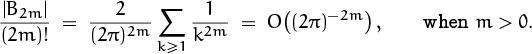
Dirichlet series, which are sums of the form Σk≥1 ak/kz, can be truncated in a similar way: If a Dirichlet series converges absolutely when z = z0, we can truncate it at any term and get the approximation
valid for ℜz ≥ ℜz0. The asymptotic formula for Bernoulli numbers Bn in Table 452 illustrates this principle.
Remember that ℜ stands for “real part.”
On the other hand, the asymptotic formulas for Hn, n!, and π(n) in Table 452 are not truncations of convergent series; if we extended them indefinitely they would diverge for all values of n. This is particularly easy to see in the case of π(n), since we have already observed in Section 7.3, Example 5, that the power series Σk≥0 k!/(ln n)k is everywhere divergent. Yet these truncations of divergent series turn out to be useful approximations.
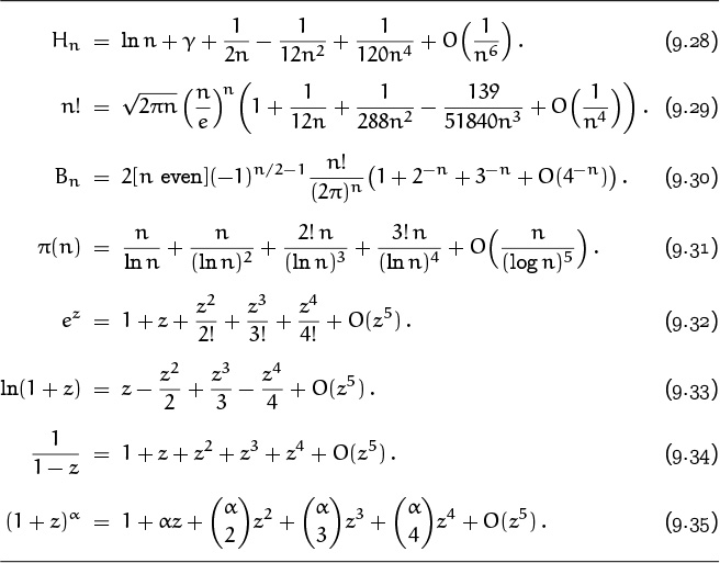
An asymptotic approximation is said to have absolute error O(g(n)) if it has the form f(n) + O(g(n)) where f(n) doesn’t involve O. The approximation has relative error O(g(n)) if it has the form f(n) (1 + O (g(n))) where f(n) doesn’t involve O. For example, the approximation for Hn in Table 452 has absolute error O(n–6); the approximation for n! has relative error O(n–4). (The right-hand side of (9.29) doesn’t actually have the required form f(n) (1 + O(n–4)), but we could rewrite it
if we wanted to; a similar calculation is the subject of exercise 12.) The absolute error of this approximation is O(nn–3.5e–n). Absolute error is related to the number of correct decimal digits to the right of the decimal point if the O term is ignored; relative error corresponds to the number of correct “significant figures.”
(Relative error is nice for taking reciprocals, because 1/(1 + O(![]() )) = 1 + O(
)) = 1 + O(![]() ).)
).)
We can use truncation of power series to prove the general laws
(Here we assume that n → ∞; similar formulas hold for ln(1 + O(f(x))) and eO(f(x)) as x → 0.) For example, let ln(1 + g(n)) be any function belonging to the left side of (9.36). Then there are constants C, n0, and c such that
| |g(n)| ≤ C|f(n)| ≤ c < 1 , | for all n ≥ n0. |
It follows that the infinite sum
converges for all n ≥ n0, and the parenthesized series is bounded by the constant ![]() . This proves (9.36), and the proof of (9.37) is similar. Equations (9.36) and (9.37) combine to give the useful formula
. This proves (9.36), and the proof of (9.37) is similar. Equations (9.36) and (9.37) combine to give the useful formula
Problem 1: Return to the Wheel of Fortune.
Let’s try our luck now at a few asymptotic problems. In Chapter 3 we derived equation (3.13) for the number of winning positions in a certain game:
And we promised that an asymptotic version of W would be derived in Chapter 9. Well, here we are in Chapter 9; let’s try to estimate W, as N → ∞.
The main idea here is to remove the floor brackets, replacing K by N1/3 + O(1). Then we can go further and write
K = N1/3 (1 + O(N–1/3));
this is called “pulling out the large part.” (We will be using this trick a lot.) Now we have
| K2 | = | N2/3(1 + O(N–1/3))2 |
| = | N2/3(1 + O(N–1/3)) = N2/3 + O(N1/3) |
by (9.38) and (9.26). Similarly
| = | N1 –1/3 (1 + O(N–1/3)) –1 + O(1) | |
| = | N2/3 (1 + O(N–1/3))+ O(1) = N2/3 + O(N1/3) . |
It follows that the number of winning positions is

Notice how the O terms absorb one another until only one remains; this is typical, and it illustrates why O-notation is useful in the middle of a formula.
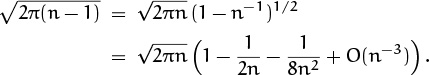
Problem 2: Perturbation of Stirling’s formula.
Stirling’s approximation for n! is undoubtedly the most famous asymptotic formula of all. We will prove it later in this chapter; for now, let’s just try to get better acquainted with its properties. We can write one version of the approximation in the form
for certain constants a and b. Since this holds for all large n, it must also be asymptotically true when n is replaced by n – 1:
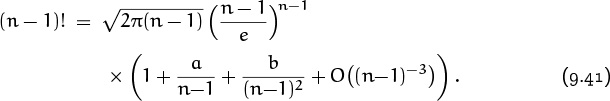
We know, of course, that (n – 1)! = n!/n; hence the right-hand side of this formula must simplify to the right-hand side of (9.40), divided by n.
Let us therefore try to simplify (9.41). The first factor becomes tractable if we pull out the large part:
Equation (9.35) has been used here.
Similarly we have

The only thing in (9.41) that’s slightly tricky to deal with is the factor (n – 1)n–1, which equals
nn–1(1 – n–1)n–1 = nn–1(1 – n–1)n (1 + n–1 + n–2 + O(n–3)).
(We are expanding everything out until we get a relative error of O(n–3), because the relative error of a product is the sum of the relative errors of the individual factors. All of the O(n–3) terms will coalesce.)
In order to expand (1 – n–1)n, we first compute ln(1 – n–1) and then form the exponential, en ln(1–n–1):
| (1 – n–1)n | = | exp (n ln(1 – n–1)) |
| = | exp (n (–n–1 – |
|
| = | exp (–1 – |
|
| = | exp(–1) · exp(– |
|
| = | exp(–1) ·( 1 – · (1 – |
|
| = | e–1 (1 – |
Here we use the notation exp z instead of ez, since it allows us to work with a complicated exponent on the main line of the formula instead of in the superscript position. We must expand ln(1–n–1) with absolute error O(n–4) in order to end with a relative error of O(n–3), because the logarithm is being multiplied by n.
The right-hand side of (9.41) has now been reduced to ![]() times nn–1/en times a product of several factors:
times nn–1/en times a product of several factors:
| ( 1 – |
|
| · (1 + n–1 + n–2 + O(n–3)) | |
| · (1 – |
|
| · (1 + an–1 + (a + b)n–2 + O(n–3)). | |
Multiplying these out and absorbing all asymptotic terms into one O(n–3) yields
1 + an–1 + (a + b – ![]() )n–2 + O(n–3) .
)n–2 + O(n–3) .
Hmmm; we were hoping to get 1 + an–1 + bn–2 + O(n–3), since that’s what we need to match the right-hand side of (9.40). Has something gone awry? No, everything is fine, provided that ![]() .
.
This perturbation argument doesn’t prove the validity of Stirling’s approximation, but it does prove something: It proves that formula (9.40) cannot be valid unless ![]() . If we had replaced the O(n–3) in (9.40) by cn–3 + O(n–4) and carried out our calculations to a relative error of O(n–4), we could have deduced that b must be
. If we had replaced the O(n–3) in (9.40) by cn–3 + O(n–4) and carried out our calculations to a relative error of O(n–4), we could have deduced that b must be ![]() , as claimed in Table 452. (This is not the easiest way to determine the values of a and b, but it works.)
, as claimed in Table 452. (This is not the easiest way to determine the values of a and b, but it works.)
Problem 3: The nth prime number.
Equation (9.31) is an asymptotic formula for π(n), the number of primes that do not exceed n. If we replace n by p = Pn, the nth prime number, we have π(p) = n; hence
as n → ∞. Let us try to “solve” this equation for p; then we will know the approximate size of the nth prime.
The first step is to simplify the O term. If we divide both sides by p/ln p, we find that n ln p/p → 1; hence p/ln p = O(n) and
(We have (log p)–1 ≤ (log n)–1 because p ≥ n.)
The second step is to transpose the two sides of (9.42), except for the O term. This is legal because of the general rule
(Each of these equations follows from the other if we multiply both sides by –1 and then add an + bn to both sides.) Hence
and we have
This is an “approximate recurrence” for p = Pn in terms of itself. Our goal is to change it into an “approximate closed form,” and we can do this by unfolding the recurrence asymptotically. So let’s try to unfold (9.44).
By taking logarithms of both sides we deduce that
This value can be substituted for ln p in (9.44), but we would like to get rid of all p’s on the right before making the substitution. Somewhere along the line, that last p must disappear; we can’t get rid of it in the normal way for recurrences, because (9.44) doesn’t specify initial conditions for small p.
One way to do the job is to start by proving the weaker result p = O(n2).
This follows if we square (9.44) and divide by pn2,
since the right side approaches zero as n → ∞. OK, we know that p = O(n2); therefore log p = O(log n) and log log p = O(log log n). We can now conclude from (9.45) that
ln p = ln n + O(log log n);
in fact, with this new estimate in hand we can conclude that ln ln p = ln ln n+ O(log log n/log n), and (9.45) now yields
ln p = ln n + ln ln n + O(log log n/log n).
And we can plug this into the right-hand side of (9.44), obtaining
p = n ln n + n ln ln n + O(n).
This is the approximate size of the nth prime.
Get out the scratch paper again, gang.
Boo, Hiss.
We can refine this estimate by using a better approximation of π(p) in place of (9.42). The next term of (9.31) tells us that
proceeding as before, we obtain the recurrence
which has a relative error of O(1/log n)2 instead of O(1/log n). Taking logarithms and retaining proper accuracy (but not too much) now yields

Finally we substitute these results into (9.47) and our answer finds its way out:
For example, when n = 106 this estimate comes to 15631363.6 + O(n/log n); the millionth prime is actually 15485863. Exercise 21 shows that a still more accurate approximation to Pn results if we begin with a still more accurate approximation to π(p) in place of (9.46).
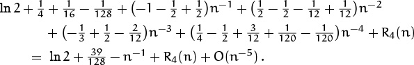
Problem 4: A sum from an old final exam.
When Concrete Mathematics was first taught at Stanford University during the 1970–1971 term, students were asked for the asymptotic value of the sum
with an absolute error of O(n–7). Let’s imagine that we’ve just been given this problem on a (take-home) final; what is our first instinctive reaction?
No, we don’t panic. Our first reaction is to THINK BIG. If we set n = 10100, say, and look at the sum, we see that it consists of n terms, each of which is slightly less than 1/n2; hence the sum is slightly less than 1/n. In general, we can usually get a decent start on an asymptotic problem by taking stock of the situation and getting a ballpark estimate of the answer.
Let’s try to improve the rough estimate by pulling out the largest part of each term. We have

and so it’s natural to try summing all these approximations:
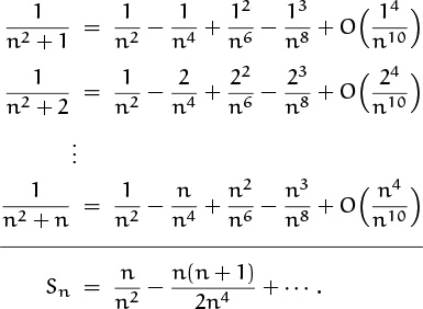
It looks as if we’re getting Sn = n–1 – ![]() n–2 + O(n–3), based on the sums of the first two columns; but the calculations are getting hairy.
n–2 + O(n–3), based on the sums of the first two columns; but the calculations are getting hairy.
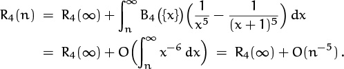
If we persevere in this approach, we will ultimately reach the goal; but we won’t bother to sum the other columns, for two reasons: First, the last column is going to give us terms that are O(n–6), when n/2 ≤ k ≤ n, so we will have an error of O(n–5); that’s too big, and we will have to include yet another column in the expansion. Could the exam-giver have been so sadistic? We suspect that there must be a better way. Second, there is indeed a much better way, staring us right in the face.
Do pajamas have buttons?
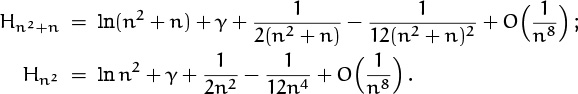
Namely, we know a closed form for Sn: It’s just Hn2+n – Hn2 . And we know a good approximation for harmonic numbers, so we just apply it twice:
Now we can pull out large terms and simplify, as we did when looking at Stirling’s approximation. We have
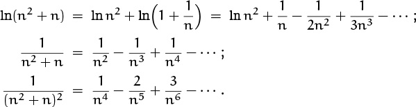
So there’s lots of helpful cancellation, and we find
| Sn = n–1 – |
| – |
| + |
plus terms that are O(n–7). A bit of arithmetic and we’re home free:
It would be nice if we could check this answer numerically, as we did when we derived exact results in earlier chapters. Asymptotic formulas are harder to verify; an arbitrarily large constant may be hiding in a O term, so any numerical test is inconclusive. But in practice, we have no reason to believe that an adversary is trying to trap us, so we can assume that the unknown O-constants are reasonably small. With a pocket calculator we find that ![]() ; and our asymptotic estimate when n = 4 comes to
; and our asymptotic estimate when n = 4 comes to
If we had made an error of, say, ![]() in the term for n–6, a difference of
in the term for n–6, a difference of ![]() would have shown up in the fifth decimal place; so our asymptotic answer is probably correct.
would have shown up in the fifth decimal place; so our asymptotic answer is probably correct.
Problem 5: An infinite sum.
We turn now to an asymptotic question posed by Solomon Golomb [152]: What is the approximate value of

where Nn(k) is the number of digits required to write k in radix n notation?
First let’s try again for a ballpark estimate. The number of digits, Nn(k), is approximately logn k = log k/log n; so the terms of this sum are roughly (log n)2/k(log k)2. Summing on k gives ≈ (log n)2 Σk≥2 1/k(log k)2, and this sum converges to a constant value because it can be compared to the integral
Therefore we expect Sn to be about C(log n)2, for some constant C.
Hand-wavy analyses like this are useful for orientation, but we need better estimates to solve the problem. One idea is to express Nn(k) exactly:
Thus, for example, k has three radix n digits when n2 ≤ k < n3, and this happens precisely when ![]() logn k
logn k![]() = 2. It follows that Nn(k) > logn k, hence Sn =Σk≥1 1/kNn(k)2 < 1 + (log n)2 Σk≥2 1/k(log k)2.
= 2. It follows that Nn(k) > logn k, hence Sn =Σk≥1 1/kNn(k)2 < 1 + (log n)2 Σk≥2 1/k(log k)2.
Proceeding as in Problem 1, we can try to write Nn(k) = logn k + O(1) and substitute this into the formula for Sn. The term represented here by O(1) is always between 0 and 1, and it is about ![]() on the average, so it seems rather well-behaved. But still, this isn’t a good enough approximation to tell us about Sn; it gives us zero significant figures (that is, high relative error) when k is small, and these are the terms that contribute the most to the sum. We need a different idea.
on the average, so it seems rather well-behaved. But still, this isn’t a good enough approximation to tell us about Sn; it gives us zero significant figures (that is, high relative error) when k is small, and these are the terms that contribute the most to the sum. We need a different idea.
The key (as in Problem 4) is to use our manipulative skills to put the sum into a more tractable form, before we resort to asymptotic estimates. We can introduce a new variable of summation, m = Nn(k):
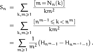
This may look worse than the sum we began with, but it’s actually a step forward, because we have very good approximations for the harmonic numbers.
Still, we hold back and try to simplify some more. No need to rush into asymptotics. Summation by parts allows us to group the terms for each value of Hnm–1 that we need to approximate:

For example, Hn2–1 is multiplied by 1/22 and then by –1/32. (We have used the fact that Hn0–1 = H0 = 0.)
Now we’re ready to expand the harmonic numbers. Our experience with estimating (n – 1)! has taught us that it will be easier to estimate Hnk than Hnk–1, since the (nk – 1)’s will be messy; therefore we write
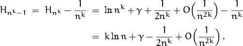
Our sum now reduces to
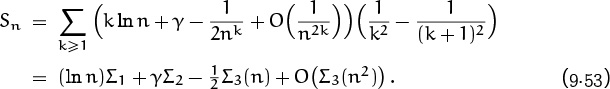
There are four easy pieces left: Σ1, Σ2, Σ3(n), and Σ3(n2).
Into a Big Oh.
Let’s do the Σ3’s first, since Σ3(n2) is the O term; then we’ll see what sort of error we’re getting. (There’s no sense carrying out other calculations with perfect accuracy if they will be absorbed into a O anyway.) This sum is simply a power series,
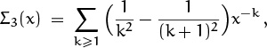
and the series converges when x ≥ 1 so we can truncate it at any desired point. If we stop Σ3(n2) at the term for k = 1, we get Σ3(n2) = O(n–2); hence (9.53) has an absolute error of O(n–2). (To decrease this absolute error, we could use a better approximation to Hnk; but O(n–2) is good enough for now.) If we truncate Σ3(n) at the term for k = 2, we get
Σ3(n) = ![]() n–1 + O(n–2);
n–1 + O(n–2);
this is all the accuracy we need.
We might as well do Σ2 now, since it is so easy:
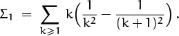
This is the telescoping series ![]() .
.
Finally, Σ1 gives us the leading term of Sn, the coefficient of ln n in (9.53):
This is ![]() . (If we hadn’t applied summation by parts earlier, we would have seen directly that Sn ∼ Σk≥1(ln n)/k2, because Hnk–1 – Hnk–1–1 ∼ ln n; so summation by parts didn’t help us to evaluate the leading term, although it did make some of our other work easier.)
. (If we hadn’t applied summation by parts earlier, we would have seen directly that Sn ∼ Σk≥1(ln n)/k2, because Hnk–1 – Hnk–1–1 ∼ ln n; so summation by parts didn’t help us to evaluate the leading term, although it did make some of our other work easier.)
Now we have evaluated each of the Σ’s in (9.53), so we can put everything together and get the answer to Golomb’s problem:
Notice that this grows more slowly than our original hand-wavy estimate of C(log n)2. Sometimes a discrete sum fails to obey a continuous intuition.
Problem 6: Big Phi.
Near the end of Chapter 4, we observed that the number of fractions in the Farey series ![]() is 1 + Φ(n), where
is 1 + Φ(n), where
Φ(n) = φ(1) + φ(2) + · · · + φ(n);
and we showed in (4.62) that

Let us now try to estimate Φ(n) when n is large. (It was sums like this that led Bachmann to invent O-notation in the first place.)
Thinking BIG tells us that Φ(n) will probably be proportional to n2. For if the final factor were just ![]() n/k
n/k![]() instead of
instead of ![]() 1 + n/k
1 + n/k![]() , we would have the upper bound | Φ(n)| ≤
, we would have the upper bound | Φ(n)| ≤ ![]() Σk≥1
Σk≥1![]() n/k
n/k![]() 2 ≤
2 ≤ ![]() Σk≥1(n/k)2 =
Σk≥1(n/k)2 = ![]() n2, because the Möbius function μ(k) is either –1, 0, or +1. The additional ‘1 + ’ in that final factor adds Σk≥1 μ(k)
n2, because the Möbius function μ(k) is either –1, 0, or +1. The additional ‘1 + ’ in that final factor adds Σk≥1 μ(k)![]() n/k
n/k![]() ; but this is zero for k > n, so it cannot be more than nHn = O(n log n) in absolute value.
; but this is zero for k > n, so it cannot be more than nHn = O(n log n) in absolute value.
This preliminary analysis indicates that we’ll find it advantageous to write
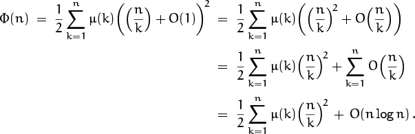
This removes the floors; the remaining problem is to evaluate the unfloored sum ![]() with an accuracy of O(n log n); in other words, we want to evaluate
with an accuracy of O(n log n); in other words, we want to evaluate ![]() with an accuracy of O(n–1 log n). But that’s easy; we can simply run the sum all the way up to k = ∞, because the newly added terms are
with an accuracy of O(n–1 log n). But that’s easy; we can simply run the sum all the way up to k = ∞, because the newly added terms are
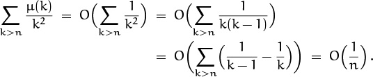
We proved in (7.89) that Σk≥1 μ(k)/kz = 1/ζ(z). Hence Σk≥1 μ(k)/k2 = 1/(Σk≥1 1/k2) = 6/π2, and we have our answer:
(The error term was shown to be at most O(n(log n)2/3 × (log log n)1+![]() ) by Saltykov in 1960 [316]. On the other hand, it is not as small as o(n(log log n)1/2), according to Montgomery [275].)
) by Saltykov in 1960 [316]. On the other hand, it is not as small as o(n(log log n)1/2), according to Montgomery [275].)
9.4 Two Asymptotic Tricks
Now that we have some facility with O manipulations, let’s look at what we’ve done from a slightly higher perspective. Then we’ll have some important weapons in our asymptotic arsenal, when we need to do battle with tougher problems.
Trick 1: Bootstrapping.
When we estimated the nth prime Pn in Problem 3 of Section 9.3, we solved an asymptotic recurrence of the form
Pn = n ln Pn (1 + O(1/log n)).
We proved that Pn = n ln n + n ln ln n + O(n) by first using the recurrence to show the weaker result O(n2). This is a special case of a general method called bootstrapping, in which we solve a recurrence asymptotically by starting with a rough estimate and plugging it into the recurrence; in this way we can often derive better and better estimates, “pulling ourselves up by our bootstraps.”
Here’s another problem that illustrates bootstrapping nicely: What is the asymptotic value of the coefficient gn = [zn] G(z) in the generating function

as n → ∞? If we differentiate this equation with respect to z, we find
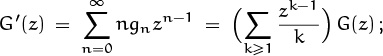
equating coefficients of zn–1 on both sides gives the recurrence
Our problem is equivalent to finding an asymptotic formula for the solution to (9.58), with the initial condition g0 = 1. The first few values
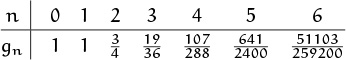
don’t reveal much of a pattern, and the integer sequence ![]() n!2gn
n!2gn![]() doesn’t appear in Sloane’s Handbook [330]; therefore a closed form for gn seems out of the question, and asymptotic information is probably the best we can hope to derive.
doesn’t appear in Sloane’s Handbook [330]; therefore a closed form for gn seems out of the question, and asymptotic information is probably the best we can hope to derive.
Our first handle on this problem is the observation that 0 < gn ≤ 1 for all n ≥ 0; this is easy to prove by induction. So we have a start:
gn = O(1).
This equation can, in fact, be used to “prime the pump” for a bootstrapping operation: Plugging it in on the right of (9.58) yields
hence we have
And we can bootstrap yet again:
obtaining
Will this go on forever? Perhaps we’ll have gn = O(n–1 log n)m for all m.
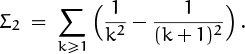
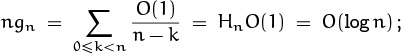
Actually no; we have just reached a point of diminishing returns. The next attempt at bootstrapping involves the sum

which is Ω(n–1); so we cannot get an estimate for gn that falls below Ω(n–2).
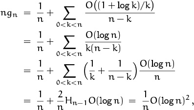
In fact, we now know enough about gn to apply our old trick of pulling out the largest part:
The first sum here is G(1) = exp( ![]() +
+ ![]() +
+ ![]() + · · · ) = eπ2/6, because G(z) converges for all |z| ≤ 1. The second sum is the tail of the first; we can get an upper bound by using (9.59):
+ · · · ) = eπ2/6, because G(z) converges for all |z| ≤ 1. The second sum is the tail of the first; we can get an upper bound by using (9.59):
This last estimate follows because, for example,

(Exercise 54 discusses a more general way to estimate such tails.)
The third sum in (9.60) is
by an argument that’s already familiar. So (9.60) proves that
Finally, we can feed this formula back into the recurrence, bootstrapping once more; the result is
(Exercise 23 peeks inside the remaining O term.)
Trick 2: Trading tails.
We derived (9.62) in somewhat the same way we derived the asymptotic value (9.56) of Φ(n): In both cases we started with a finite sum but got an asymptotic value by considering an infinite sum. We couldn’t simply get the infinite sum by introducing O into the summand; we had to be careful to use one approach when k was small and another when k was large.
(This important method was pioneered by Laplace [240].)
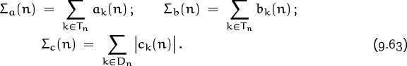
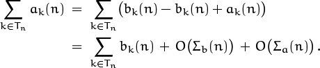
Those derivations were special cases of an important three-step asymptotic summation method we will now discuss in greater generality. Whenever we want to estimate the value of Σk ak(n), we can try the following approach:
1 First break the sum into two disjoint ranges, Dn and Tn. The summation over Dn should be the “dominant” part, in the sense that it includes enough terms to determine the significant digits of the sum, when n is large. The summation over the other range Tn should be just the “tail” end, which contributes little to the overall total.
2 Find an asymptotic estimate
ak(n) = bk(n) + O(ck(n))
that is valid when k ![]() Dn. The O bound need not hold when k
Dn. The O bound need not hold when k ![]() Tn.
Tn.
3 Now prove that each of the following three sums is small:
If all three steps can be completed successfully, we have a good estimate:
Here’s why. We can “chop off” the tail of the given sum, getting a good estimate in the range Dn where a good estimate is necessary:
And we can replace the tail with another one, even though the new tail might be a terrible approximation to the old, because the tails don’t really matter:
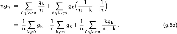
When we evaluated the sum in (9.60), for example, we had
| ak(n) | = | [0 ≤ k < n]gk/(n – k), |
| bk(n) | = | gk/n, |
| ck(n) | = | kgk/n(n – k) ; |
the ranges of summation were
| Dn = {0, 1, . . . , n – 1}, | Tn = {n, n + 1, . . . } ; |
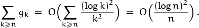
and we found that
Σa(n) = 0, Σb(n) = O ((log n)2/n2), Σc(n) = O((log n)3/n2).
This led to (9.61).
Similarly, when we estimated Φ(n) in (9.55) we had
ak(n) = µ(k)![]() n/k
n/k![]()
![]() 1+n/k
1+n/k![]() , bk(n) = µ(k)n2/k2, ck(n) = n/k;
, bk(n) = µ(k)n2/k2, ck(n) = n/k;
Dn = {1, 2, . . . , n}, Tn = {n + 1, n + 2, . . . } .
We derived (9.56) by observing that Σa(n) = 0, Σb(n) = O(n), and Σc(n) = O(n log n).
Asymptotics is the art of knowing where to be sloppy and where to be precise.
Also, horses switch their tails when feeding time approaches.
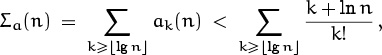
Here’s another example where tail switching is effective. (Unlike our previous examples, this one illustrates the trick in its full generality, with Σa(n) ≠ 0.) We seek the asymptotic value of
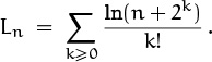
The big contributions to this sum occur when k is small, because of the k! in the denominator. In this range we have
We can prove that this estimate holds for 0 ≤ k < ![]() lg n
lg n![]() , since the original terms that have been truncated with O are bounded by the convergent series
, since the original terms that have been truncated with O are bounded by the convergent series

(In this range, ![]() .)
.)
Therefore we can apply the three-step method just described, with
| ak(n) | = | ln(n + 2k)/k!, |
| bk(n) | = | (ln n + 2k/n – 4k/2n2)/k!, |
| ck(n) | = | 8k/n3k! ; |
| Dn | = | {0, 1, . . . , |
| Tn | = | { |
All we have to do is find good bounds on the three Σ’s in (9.63), and we’ll know that Σk≥0 ak(n) ≈ Σk≥0 bk(n).
The error we have committed in the dominant part of the sum, Σc(n) = Σk![]() Dn 8k/n3k!, is obviously bounded by Σk≥0 8k/n3k! = e8/n3, so it can be replaced by O(n–3). The new tail error is
Dn 8k/n3k!, is obviously bounded by Σk≥0 8k/n3k! = e8/n3, so it can be replaced by O(n–3). The new tail error is
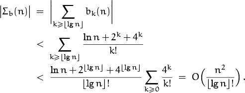
“We may not be big, but we’re small.”
Since ![]() lg n
lg n![]() ! grows faster than any power of n, this minuscule error is over-whelmed by Σc(n) = O(n–3). The error that comes from the original tail,
! grows faster than any power of n, this minuscule error is over-whelmed by Σc(n) = O(n–3). The error that comes from the original tail,
is smaller yet.
Finally, it’s easy to sum Σk≥0 bk(n) in closed form, and we have obtained the desired asymptotic formula:

The method we’ve used makes it clear that, in fact,

for any fixed m > 0. (This is a truncation of a series that diverges for all fixed n if we let m → ∞ .)
There’s only one flaw in our solution: We were too cautious. We derived (9.64) on the assumption that k < ![]() lg n
lg n![]() , but exercise 53 proves that the stated estimate is actually valid for all values of k. If we had known the stronger general result, we wouldn’t have had to use the two-tail trick; we could have gone directly to the final formula! But later we’ll encounter problems where exchange of tails is the only decent approach available.
, but exercise 53 proves that the stated estimate is actually valid for all values of k. If we had known the stronger general result, we wouldn’t have had to use the two-tail trick; we could have gone directly to the final formula! But later we’ll encounter problems where exchange of tails is the only decent approach available.
9.5 Euler’s Summation Formula
And now for our next trick—which is, in fact, the last important technique that will be discussed in this book—we turn to a general method of approximating sums that was first published by Leonhard Euler [101] in 1732. (The idea is sometimes also associated with the name of Colin Maclaurin, a professor of mathematics at Edinburgh who discovered it independently a short time later [263, page 305].)
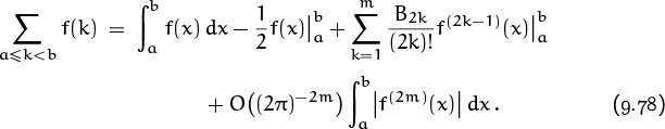
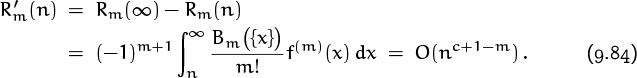
Here’s the formula:

On the left is a typical sum that we might want to evaluate. On the right is another expression for that sum, involving integrals and derivatives. If f(x) is a sufficiently “smooth” function, it will have m derivatives f′(x), . . . , f(m) (x), and this formula turns out to be an identity. The right-hand side is often an excellent approximation to the sum on the left, in the sense that the remainder Rm is often small. For example, we’ll see that Stirling’s approximation for n! is a consequence of Euler’s summation formula; so is our asymptotic approximation for the harmonic number Hn.
The numbers Bk in (9.67) are the Bernoulli numbers that we met in Chapter 6; the function Bm ({x}) in (9.68) is the Bernoulli polynomial that we met in Chapter 7. The notation {x} stands for the fractional part x – ![]() x
x![]() , as in Chapter 3. Euler’s summation formula sort of brings everything together.
, as in Chapter 3. Euler’s summation formula sort of brings everything together.
Let’s recall the values of small Bernoulli numbers, since it’s always handy to have them listed near Euler’s general formula:
B0 = 1, B1 = –![]() , B2 =
, B2 = ![]() , B4 = –
, B4 = – ![]() , B6 =
, B6 = ![]() , B8 = –
, B8 = – ![]() ;
;
B3 = B5 = B7 = B9 = B11 = · · · = 0.
Jakob Bernoulli discovered these numbers when studying the sums of powers of integers, and Euler’s formula explains why: If we set f(x) = xm–1, we have f(m)(x) = 0; hence Rm = 0, and (9.67) reduces to

For example, when m = 3 we have our favorite example of summation:

(This is the last time we shall derive this famous formula in this book.)
All good things must come to an end.
Before we prove Euler’s formula, let’s look at a high-level reason (due to Lagrange [234]) why such a formula ought to exist. Chapter 2 defines the difference operator Δ and explains that Σ is the inverse of Δ, just as ∫ is the inverse of the derivative operator D. We can express Δ in terms of D using Taylor’s formula as follows:
f(x + ![]() ) = f(x) +
) = f(x) + ![]()
![]() +
+ ![]()
![]() 2 + · · · .
2 + · · · .
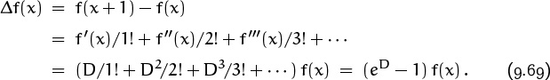
Here eD stands for the differential operation 1 + D/1! + D2/2! + D3/3! + · · · . Since Δ = eD – 1, the inverse operator Σ = 1/Δ should be 1/(eD – 1); and we know from Table 351 that z/(ez – 1) = Σk≥0 Bkzk/k! is a power series involving Bernoulli numbers. Thus

Applying this operator equation to f(x) and attaching limits yields

which is exactly Euler’s summation formula (9.67) without the remainder term. (Euler did not, in fact, consider the remainder, nor did anybody else until S. D. Poisson [295] published an important memoir about approximate summation in 1823. The remainder term is important, because the infinite sum ![]() often diverges. Our derivation of (9.71) has been purely formal, without regard to convergence.)
often diverges. Our derivation of (9.71) has been purely formal, without regard to convergence.)
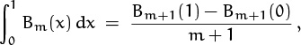
Now let’s prove (9.67), with the remainder included. It suffices to prove the case a = 0 and b = 1, namely

because we can then replace f(x) by f(x + l) for any integer l, getting

The general formula (9.67) is just the sum of this identity over the range a ≤ l < b, because intermediate terms telescope nicely.
The proof when a = 0 and b = 1 is by induction on m, starting with m = 1:
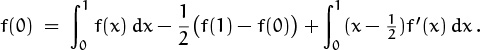
(The Bernoulli polynomial Bm(x) is defined by the equation
in general, hence B1(x) = x – ![]() in particular.) In other words, we want to prove that
in particular.) In other words, we want to prove that
But this is just a special case of the formula
for integration by parts, with u(x) = f(x) and v(x) = x – ![]() . Hence the case m = 1 is easy.
. Hence the case m = 1 is easy.
Will the authors never get serious?
To pass from m – 1 to m and complete the induction when m > 1, we need to show that ![]() , namely that
, namely that
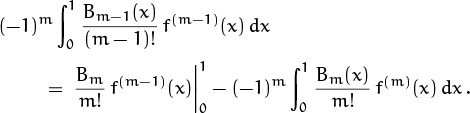
This reduces to the equation

Once again (9.73) applies to these two integrals, with u(x) = f(m–1)(x) and v(x) = Bm(x), because the derivative of the Bernoulli polynomial (9.72) is
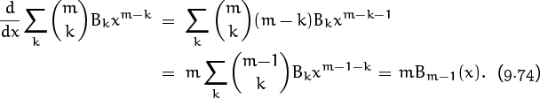
(The absorption identity (5.7) was useful here.) Therefore the required formula will hold if and only if
In other words, we need to have
This is a bit embarrassing, because Bm(0) is obviously equal to Bm, not to (–1)mBm. But there’s no problem really, because m > 1; we know that Bm is zero when m is odd. (Still, that was a close call.)
To complete the proof of Euler’s summation formula we need to show that Bm(1) = Bm(0), which is the same as saying that
 Bk = Bm, for m > 1.
But this is just the definition of Bernoulli numbers, (6.79), so we’re done.
The identity ![]() = mBm–1(x) implies that
= mBm–1(x) implies that
and we know now that this integral is zero when m ≥ 1. Hence the remainder term in Euler’s formula,
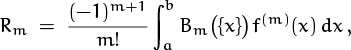
multiplies f(m)(x) by a function Bm ({x}) whose average value is zero. This means that Rm has a reasonable chance of being small.
Let’s look more closely at Bm(x) for 0 ≤ x ≤ 1, since Bm(x) governs the behavior of Rm. Here are the graphs for Bm(x) for the first twelve values of m:
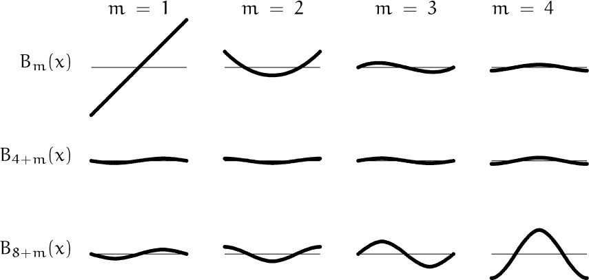
Although B3(x) through B9(x) are quite small, the Bernoulli polynomials and numbers ultimately get quite large. Fortunately Rm has a compensating factor 1/m!, which helps to calm things down.
The graph of Bm(x) begins to look very much like a sine wave when m ≥ 3; exercise 58 proves that Bm(x) can in fact be well approximated by a negative multiple of cos(2πx – ![]() πm), with error O(2–m maxx Bm ({x})).
πm), with error O(2–m maxx Bm ({x})).
In general, B4k+1(x) is negative for for 0 < x < ![]() and positive for
and positive for ![]() < x < 1. Therefore its integral, B4k+2(x)/(4k+2), decreases for 0 < x <
< x < 1. Therefore its integral, B4k+2(x)/(4k+2), decreases for 0 < x < ![]() and increases for
and increases for ![]() < x < 1. Moreover, we have
< x < 1. Moreover, we have
B4k+1(1 – x) = –B4k+1(x), for 0 ≤ x ≤ 1,
and it follows that
B4k+2(1 – x) = B4k+2(x), for 0 ≤ x ≤ 1.
The constant term B4k+2 causes the integral ![]() to be zero; hence B4k+2 > 0. The integral of B4k+2(x) is B4k+3(x)/(4k + 3), which must therefore be positive when 0 < x <
to be zero; hence B4k+2 > 0. The integral of B4k+2(x) is B4k+3(x)/(4k + 3), which must therefore be positive when 0 < x < ![]() and negative when
and negative when ![]() < x < 1; furthermore B4k+3(1–x) = –B4k+3(x), so B4k+3(x) has the properties stated for B4k+1(x), but negated. Therefore B4k+4(x) has the properties stated for B4k+2(x), but negated. Therefore B4k+5(x) has the properties stated for B4k+1(x); we have completed a cycle that establishes the stated properties inductively for all k.
< x < 1; furthermore B4k+3(1–x) = –B4k+3(x), so B4k+3(x) has the properties stated for B4k+1(x), but negated. Therefore B4k+4(x) has the properties stated for B4k+2(x), but negated. Therefore B4k+5(x) has the properties stated for B4k+1(x); we have completed a cycle that establishes the stated properties inductively for all k.
According to this analysis, the maximum value of B2m(x) must occur either at x = 0 or at x = ![]() . Exercise 17 proves that
. Exercise 17 proves that
hence we have
This can be used to establish a useful upper bound on the remainder in Euler’s summation formula, because we know from (6.89) that
Therefore we can rewrite Euler’s formula (9.67) as follows:
For example, if f(x) = ex, all derivatives are the same and this formula tells us that ![]() ek = (eb – ea) (1 –
ek = (eb – ea) (1 – ![]() + B2/2! + B4/4! + · · · + B2m/(2m)!+ O (2π)–2m . Of course, we know that this sum is actually a geometric series, equal to (eb – ea)/(e – 1) = (eb – ea) Σk≥0 Bk/k!.
+ B2/2! + B4/4! + · · · + B2m/(2m)!+ O (2π)–2m . Of course, we know that this sum is actually a geometric series, equal to (eb – ea)/(e – 1) = (eb – ea) Σk≥0 Bk/k!.
If f(2m)(x) ≥ 0 for a ≤ x ≤ b, the integral ![]() is just
is just ![]() , so we have
, so we have
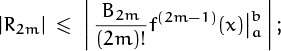
in other words, the remainder is bounded by the magnitude of the final term (the term just before the remainder), in this case. We can give an even better estimate if we know that
For it turns out that this implies the relation
in other words, the remainder will then lie between 0 and the first discarded term in (9.78)—the term that would follow the final term if we increased m.
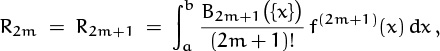
Here’s the proof: Euler’s summation formula is valid for all m, and B2m+1 = 0 when m > 0; hence R2m = R2m+1, and the first discarded term must be
R2m – R2m+2.
We therefore want to show that R2m lies between 0 and R2m – R2m+2; and this is true if and only if R2m and R2m+2 have opposite signs. We claim that
This, together with (9.79), will prove that R2m and R2m+2 have opposite signs, so the proof of (9.80) will be complete.
It’s not difficult to prove (9.81) if we recall the definition of R2m+1 and the facts we proved about the graph of B2m+1(x). Namely, we have
and f(2m+1) (x) is increasing because its derivative f(2m+2) (x) is positive. (More precisely, f(2m+1) (x) is nondecreasing because its derivative is nonnegative.) The graph of B2m+1 ({x}) looks like (–1)m+1 times a sine wave, so it is geometrically obvious that the second half of each sine wave is more influential than the first half when it is multiplied by an increasing function. This makes (–1)mR2m+1 ≥ 0, as desired. Exercise 16 proves the result formally.
9.6 Final Summations
Now comes the summing up, as we prepare to conclude this book. We will apply Euler’s summation formula to some interesting and important examples.
Summation 1: This one is too easy.
But first we will consider an interesting unimportant example, namely a sum that we already know how to do. Let’s see what Euler’s summation formula tells us if we apply it to the telescoping sum

It can’t hurt to embark on our first serious application of Euler’s formula with the asymptotic equivalent of training wheels.
We might as well start by writing the function f(x) = 1/x(x+1) in partial fraction form,
since this makes it easier to integrate and differentiate. Indeed, we have f′(x) = –1/x2 + 1/(x + 1)2 and f″(x) = 2/x3 – 2/(x + 1)3; in general
Furthermore
Plugging this into the summation formula (9.67) gives

where ![]() .
.
For example, the right-hand side when m = 4 is
This is kind of a mess; it certainly doesn’t look like the real answer 1 – n–1. But let’s keep going anyway, to see what we’ve got. We know how to expand the right-hand terms in negative powers of n up to, say, O(n–5):
| = | –n–1 + |
|
| = | n–1 – n–2 + n–3 – n–4 + O(n–5); | |
| = | n–2 – 2n–3 + 3n–4 + O(n–5); | |
| = | n–4 + O(n–5) . |
Therefore the terms on the right of our approximation add up to
The coefficients of n–2, n–3, and n–4 cancel nicely, as they should.
If all were well with the world, we would be able to show that R4(n) is asymptotically small, maybe O(n–5), and we would have an approximation to the sum. But we can’t possibly show this, because we happen to know that the correct constant term is 1, not ln 2 + ![]() (which is approximately 0.9978). So R4(n) is actually equal to
(which is approximately 0.9978). So R4(n) is actually equal to ![]() – ln 2 + O(n–5), but Euler’s summation formula doesn’t tell us this.
– ln 2 + O(n–5), but Euler’s summation formula doesn’t tell us this.
In other words, we lose.
One way to try fixing things is to notice that the constant terms in the approximation form a pattern, if we let m get larger and larger:
Perhaps we can show that this series approaches 1 as the number of terms becomes infinite? But no; the Bernoulli numbers get very large. For example, ![]() ; therefore |R22(n)| will be much larger than |R4(n)|. We lose totally.
; therefore |R22(n)| will be much larger than |R4(n)|. We lose totally.
There is a way out, however, and this escape route will turn out to be important in other applications of Euler’s formula. The key is to notice that R4(n) approaches a definite limit as n → ∞:
The integral ![]() will exist whenever f(m)(x) = O(x–2) as x → ∞, and in this case f(4)(x) surely qualifies. Moreover, we have
will exist whenever f(m)(x) = O(x–2) as x → ∞, and in this case f(4)(x) surely qualifies. Moreover, we have
Thus we have used Euler’s summation formula to prove that
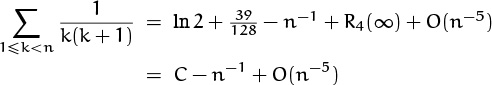
for some constant C. We do not know what the constant is—some other method must be used to establish it—but Euler’s summation formula is able to let us deduce that the constant exists.
Suppose we had chosen a much larger value of m. Then the same reasoning would tell us that
Rm(n) = Rm(∞) + O(n–m–1),
and we would have the formula

for certain constants c2, c3, . . . . We know that the c’s happen to be zero in this case; but let’s prove it, just to restore some of our confidence (in Euler’s formula if not in ourselves). The term ln ![]() contributes (–1)m/m to cm; the term (–1)m+1(Bm/m)n–m contributes (–1)m+1 Bm/m; and the term (–1)k(Bk/k)(n + 1)–k contributes
contributes (–1)m/m to cm; the term (–1)m+1(Bm/m)n–m contributes (–1)m+1 Bm/m; and the term (–1)k(Bk/k)(n + 1)–k contributes ![]() . Therefore
. Therefore
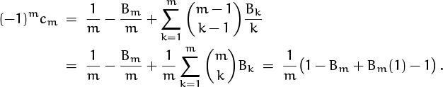
Sure enough, it’s zero, when m > 1. We have proved that

This is not enough to prove that the sum is exactly equal to C – n–1; the actual value might be C – n–1 + 2–n or something. But Euler’s summation formula does give us the error bound O(n–m–1) for arbitrarily large m, even though we haven’t evaluated any remainders explicitly.
Summation 1, again: Recapitulation and generalization.
Before we leave our training wheels, let’s review what we just did from a somewhat higher perspective. We began with a sum
and we used Euler’s summation formula to write

where F(x) was ∫ f(x) dx and where Tk(x) was a certain term involving Bk and f(k–1)(x). We also noticed that there was a constant c such that
f(m)(x) = O(xc–m) as x → ∞, for all large m.
Namely, f(k) was 1/k(k + 1); F(x) was ln(x/(x + 1)); c was –2; and Tk(x) was (–1)k+1(Bk/k) (x–k – (x + 1)–k). For all large enough values of m, this implied that the remainders had a small tail,
Therefore we were able to conclude that there exists a constant C such that

(Notice that C nicely absorbed the Tk(1) terms, which were a nuisance.)
We can save ourselves unnecessary work in future problems by simply asserting the existence of C whenever Rm(∞) exists.
Now let’s suppose that f(2m+2)(x) ≥ 0 and f(2m+4)(x) ≥ 0 for 1 ≤ x ≤ n. We have proved that this implies a simple bound (9.80) on the remainder,
R2m(n) = θm,n (T2m+2(n) – T2m+2(1)),
where θm,n lies somewhere between 0 and 1. But we don’t really want bounds that involve R2m(n) and T2m+2(1); after all, we got rid of Tk(1) when we introduced the constant C. What we really want is a bound like
![]() = ϕm,nT2m+2(n),
= ϕm,nT2m+2(n),
where 0 < ϕm,n < 1; this will allow us to conclude from (9.85) that

hence the remainder will truly be between zero and the first discarded term.
A slight modification of our previous argument will patch things up perfectly. Let us assume that
The right-hand side of (9.85) is just like the negative of the right-hand side of Euler’s summation formula (9.67) with a = n and b = ∞, as far as remainder terms are concerned, and successive remainders are generated by induction on m. Therefore our previous argument can be applied.
Summation 2: Harmonic numbers harmonized.
Now that we’ve learned so much from a trivial (but safe) example, we can readily do a nontrivial one. Let us use Euler’s summation formula to derive the approximation for Hn that we have been claiming for some time.
In this case, f(x) = 1/x. We already know about the integral and derivatives of f, because of Summation 1; also f(m)(x) = O(x–m–1) as x → ∞.
Therefore we can immediately plug into formula (9.85):

for some constant C. The sum on the left is Hn–1, not Hn; but it’s more convenient to work with Hn–1 and to add 1/n later, than to mess around with (n + 1)’s on the right-hand side. The B1n–1 will then become (B1 + 1)n–1 = 1/(2n). Let us call the constant γ instead of C, since Euler’s constant γ is, in fact, defined to be limn→∞(Hn – ln n).
The remainder term can be estimated nicely by the theory we developed a minute ago, because f(2m)(x) = (2m)!/x2m+1 ≥ 0 for all x > 0. Therefore (9.86) tells us that

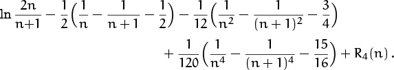
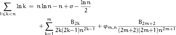
where θm,n is some fraction between 0 and 1. This is the general formula whose first few terms are listed in Table 452. For example, when m = 2 we get
This equation, incidentally, gives us a good approximation to γ even when n = 2:
γ = H2 – ln 2 – ![]() +
+ ![]() –
– ![]() +
+ ![]() = 0.577165 . . . +
= 0.577165 . . . + ![]() ,
,
where ![]() is between zero and
is between zero and ![]() . If we take n = 104 and m = 250, we get the value of γ correct to 1271 decimal places, beginning thus:
. If we take n = 104 and m = 250, we get the value of γ correct to 1271 decimal places, beginning thus:
But Euler’s constant appears also in other formulas that allow it to be evaluated even more efficiently [345].
Summation 3: Stirling’s approximation.
If f(x) = ln x, we have f′(x) = 1/x, so we can evaluate the sum of logarithms using almost the same calculations as we did when summing reciprocals. Euler’s summation formula yields
where σ is a certain constant, “Stirling’s constant,” and 0 < φm,n < 1. (In this case f(2m)(x) is negative, not positive; but we can still say that the remainder is governed by the first discarded term, because we could have started with f(x) = – ln x instead of f(x) = ln x.) Adding ln n to both sides gives
when m = 2. And we can get the approximation in Table 452 by taking ‘exp’ of both sides. (The value of eσ turns out to be ![]() , but we aren’t quite ready to derive that formula. In fact, Stirling didn’t discover the closed form for σ until several years after de Moivre [76] had proved that the constant exists.)
, but we aren’t quite ready to derive that formula. In fact, Stirling didn’t discover the closed form for σ until several years after de Moivre [76] had proved that the constant exists.)
If m is fixed and n → ∞, the general formula gives a better and better approximation to ln n! in the sense of absolute error, hence it gives a better and better approximation to n! in the sense of relative error. But if n is fixed and m increases, the error bound |B2m+2|/(2m + 2)(2m + 1)n2m+1 decreases to a certain point and then begins to increase. Therefore the approximation reaches a point beyond which a sort of uncertainty principle limits the amount by which n! can be approximated.
Heisenberg may have been here.
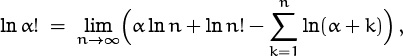
In Chapter 5, equation (5.83), we generalized factorials to arbitrary real α by using a definition
suggested by Euler. Suppose α is a large number; then
and Euler’s summation formula can be used with f(x) = ln(x + α) to estimate this sum:
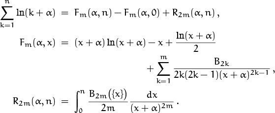
(Here we have used (9.67) with a = 0 and b = n, then added ln(n + α) – ln α to both sides.) If we subtract this approximation for ![]() from Stirling’s approximation for ln n!, then add α ln n and take the limit as n → ∞, we get
from Stirling’s approximation for ln n!, then add α ln n and take the limit as n → ∞, we get

because α ln n+n ln n–n+ ![]() ln n–(n+α) ln(n+α)+n–
ln n–(n+α) ln(n+α)+n– ![]() ln(n+α) → –α and the other terms not shown here tend to zero. Thus Stirling’s approximation behaves for generalized factorials (and for the Gamma function Γ(α + 1) = α!) exactly as for ordinary factorials.
ln(n+α) → –α and the other terms not shown here tend to zero. Thus Stirling’s approximation behaves for generalized factorials (and for the Gamma function Γ(α + 1) = α!) exactly as for ordinary factorials.
Summation 4: A bell-shaped summand.
Let’s turn now to a sum that has quite a different flavor:

This is a doubly infinite sum, whose terms reach their maximum value e0 = 1 when k = 0. We call it Θn because it is a power series involving the quantity e–1/n raised to the p(k)th power, where p(k) is a polynomial of degree 2; such power series are traditionally called “theta functions.” If n = 10100, we have

So the summand stays very near 1 until k gets up to about ![]() , when it drops off and stays very near zero. We can guess that Θn will be proportional to
, when it drops off and stays very near zero. We can guess that Θn will be proportional to ![]() . Here is a graph of e–k2/n when n = 10:
. Here is a graph of e–k2/n when n = 10:
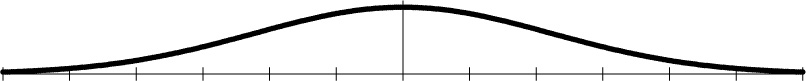
Larger values of n just stretch the graph horizontally by a factor of ![]() .
.
We can estimate Θn by letting f(x) = e–x2/n and taking a = –∞, b = + ∞ in Euler’s summation formula. (If infinities seem too scary, let a = –A and b = +B, then take limits as A, B → ∞.) The integral of f(x) is
if we replace x by ![]() . The value of
. The value of ![]() du is well known, but we’ll call it C for now and come back to it after we have finished plugging into Euler’s summation formula.
du is well known, but we’ll call it C for now and come back to it after we have finished plugging into Euler’s summation formula.
The next thing we need to know is the sequence of derivatives f′(x), f″(x), . . . , and for this purpose it’s convenient to set
Then the chain rule of calculus says that
and this is the same as saying that
By induction we have
For example, we have g′(x) = –2xe–x2 and g″(x) = (4x2 – 2)e–x2 ; hence
It’s easier to see what’s going on if we work with the simpler function g(x).
We don’t have to evaluate the derivatives of g(x) exactly, because we’re only going to be concerned about the limiting values when x = ±∞. And for this purpose it suffices to notice that every derivative of g(x) is e–x2 times a polynomial in x:
g(k)(x) = Pk(x)e–x2, where Pk is a polynomial of degree k.
This follows by induction.
The negative exponential e–x2 goes to zero much faster than Pk(x) goes to infinity, when x → ±, ∞ so we have
f(k)(+∞) = f(k) (–∞) = 0
for all k ≥ 0. Therefore all of the terms
vanish, and we are left with the term from ∫ f(x) dx and the remainder:
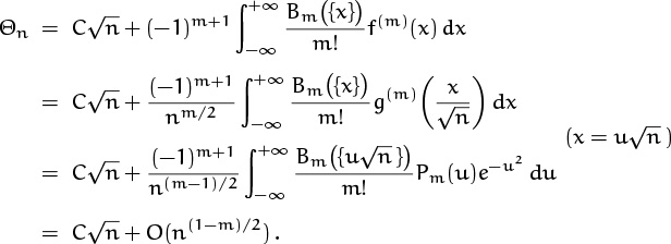
The O estimate here follows since ![]() is bounded and the integral
is bounded and the integral ![]() exists whenever P is a polynomial. (The constant implied by this O depends on m.)
exists whenever P is a polynomial. (The constant implied by this O depends on m.)
We have proved that ![]() , for arbitrarily large M; the difference between Θn and
, for arbitrarily large M; the difference between Θn and ![]() is “exponentially small.” Let us therefore determine the constant C that plays such a big role in the value of Θn.
is “exponentially small.” Let us therefore determine the constant C that plays such a big role in the value of Θn.
One way to determine C is to look the integral up in a table; but we prefer to know how the value can be derived, so that we can do integrals even when they haven’t been tabulated. Elementary calculus suffices to evaluate C if we are clever enough to look at the double integral

Converting to polar coordinates gives
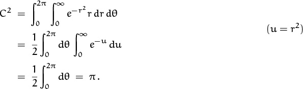
So ![]() . The fact that x2 + y2 = r2 is the equation of a circle whose circumference is 2πr somehow explains why π gets into the act.
. The fact that x2 + y2 = r2 is the equation of a circle whose circumference is 2πr somehow explains why π gets into the act.
Another way to evaluate C is to replace x by ![]() and dx by
and dx by ![]() t–1/2 dt:
t–1/2 dt:
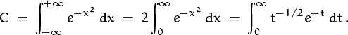
This integral equals ![]() , since
, since ![]() according to (5.84).
according to (5.84).
Therefore we have demonstrated that ![]() .
.
Our final formula, then, is
The constant in the O depends on M; that’s why we say that M is “fixed.”
When n = 2, for example, the infinite sum Θ2 is approximately equal to 2.506628288; this is already very close to ![]() ≈ 2.506628275, even though n is quite small. The value of Θ100 agrees with
≈ 2.506628275, even though n is quite small. The value of Θ100 agrees with ![]() to 427 decimal places! Exercise 59 uses advanced methods to derive a rapidly convergent series for Θn; it turns out that
to 427 decimal places! Exercise 59 uses advanced methods to derive a rapidly convergent series for Θn; it turns out that
Summation 5: The clincher.
Now we will do one last sum, which will turn out to tell us the value of Stirling’s constant σ. This last sum also illustrates many of the other techniques of this last chapter (and of this whole book), so it will be a fitting way for us to conclude our explorations of Concrete Mathematics.
The final task seems almost absurdly easy: We will try to find the asymptotic value of
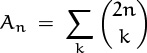
by using Euler’s summation formula.
This is another case where we already know the answer (right?); but it’s always interesting to try new methods on old problems, so that we can compare facts and maybe discover something new.
So we THINK BIG and realize that the main contribution to An comes from the middle terms, near k = n. It’s almost always a good idea to choose notation so that the biggest contribution to a sum occurs near k = 0, because we can then use the tail-exchange trick to get rid of terms that have large |k|. Therefore we replace k by n + k:
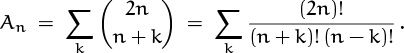
Things are looking reasonably good, since we know how to approximate (n ± k)! when n is large and k is small.
Now we want to carry out the three-step procedure associated with the tail-exchange trick. Namely, we want to write
![]() = ak(n) = bk(n) + O ck(n), for k
= ak(n) = bk(n) + O ck(n), for k ![]() Dn,
Dn,
so that we can obtain the estimate

Let us therefore try to estimate ![]() in the region where |k| is small. We could use Stirling’s approximation as it appears in Table 452, but it’s easier to work with the logarithmic equivalent in (9.91):
in the region where |k| is small. We could use Stirling’s approximation as it appears in Table 452, but it’s easier to work with the logarithmic equivalent in (9.91):

We want to convert this to a nice, simple O estimate.
The tail-exchange method allows us to work with estimates that are valid only when k is in the “dominant” set Dn. But how should we define Dn?
Actually I’m not into dominance.
We have to make Dn small enough that we can make a good estimate; for example, we had better not let k get near n, or the term O((n – k)–1) in (9.95) will blow up. Yet Dn must be large enough that the tail terms (the terms with k ∉ Dn) are negligibly small compared with the overall sum. Trial and error is usually necessary to find an appropriate set Dn; in this problem the calculations we are about to make will show that it’s wise to define things as follows:
Here ![]() is a small positive constant that we can choose later, after we get to know the territory. (Our O estimates will depend on the value of
is a small positive constant that we can choose later, after we get to know the territory. (Our O estimates will depend on the value of ![]() .) Equation (9.95) now reduces to
.) Equation (9.95) now reduces to

(We have pulled out the large parts of the logarithms, writing
ln(n ± k) = ln n + ln(1 ± k/n),
and this has made a lot of ln n terms cancel out.)
Now we need to expand the terms ln(1 ± k/n) asymptotically, until we have an error term that approaches zero as n → ∞. We are multiplying ln(1 ± k/n) by (1 ± k + ![]() ), so we should expand the logarithm until we reach o(n–1), using the assumption that |k| ≤ n1/2+
), so we should expand the logarithm until we reach o(n–1), using the assumption that |k| ≤ n1/2+![]() :
:
Multiplication by 1 ± k + ![]() yields
yields
plus other terms that are absorbed in the O(n–1/2+3![]() ). So (9.97) becomes
). So (9.97) becomes
ln ak(n) = (2n +![]() ) ln 2 – σ –
) ln 2 – σ – ![]() ln n – k2/n + O(n–1/2+3
ln n – k2/n + O(n–1/2+3![]() ) .
) .
Taking exponentials, we have
This is our approximation, with
![]() , ck(n) = 22n n–1+3
, ck(n) = 22n n–1+3![]() e–k2/n .
e–k2/n .
Notice that k enters bk(n) and ck(n) in a very simple way. We’re in luck, because we will be summing over k.
The tail-exchange trick tells us that Σk ak(n) will be approximately Σk bk(n) if we have done a good job of estimation. Let us therefore evaluate
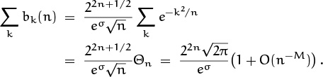
(Another stroke of luck: We get to use the sum Θn from the previous example.) This is encouraging, because we know that the original sum is actually
An = = (1 + 1)2n = 22n .
Therefore it looks as if we will have eσ = ![]() , as advertised.
, as advertised.
What an amazing coincidence.
But there’s a catch: We still need to prove that our estimates are good enough. So let’s look first at the error contributed by ck(n):
Good; this is asymptotically smaller than the previous sum, if 3![]() <
< ![]() .
.
I’m tired of getting to the end of long, hard books and not even getting a word of good wishes from the author. It would be nice to read a “thanks for reading this, hope it comes in handy,” instead of just running into a hard, cold, cardboard cover at the end of a long, dry proof. You know?
Next we must check the tails. We have

which is O(n–M) for all M; so Σk∉Dn bk(n) is asymptotically negligible. (We chose the cutoff at n1/2+![]() just so that e–k2/n would be exponentially small outside of Dn. Other choices like n1/2 log n would have been good enough too, and the resulting estimates would have been slightly sharper, but the formulas would have come out more complicated. We need not make the strongest possible estimates, since our main goal is to establish the value of the constant σ.) Similarly, the other tail
just so that e–k2/n would be exponentially small outside of Dn. Other choices like n1/2 log n would have been good enough too, and the resulting estimates would have been slightly sharper, but the formulas would have come out more complicated. We need not make the strongest possible estimates, since our main goal is to establish the value of the constant σ.) Similarly, the other tail
is bounded by 2n times its largest term, which occurs at the cutoff point k ≈ n1/2+![]() . This term is known to be approximately bk(n), which is exponentially small compared with An; and an exponentially small multiplier wipes out the factor of 2n.
. This term is known to be approximately bk(n), which is exponentially small compared with An; and an exponentially small multiplier wipes out the factor of 2n.
Thus we have successfully applied the tail-exchange trick to prove the estimate

We may choose ![]() =
= ![]() and conclude that
and conclude that
σ = ![]() ln 2π.
ln 2π.
QED.
Thanks for reading this, hope it comes in handy.
—The authors
Exercises
Warmups
1. Prove or disprove: If f1(n) ≺ g1(n) and f2(n) ≺ g2(n), then we have f1(n) + f2(n) ≺ g1(n) + g2(n).
2. Which function grows faster:
a. n(ln n) or (ln n)n?
b. n(ln ln ln n) or (ln n)!?
c. (n!)! or ((n – 1)!) ! (n – 1)!n!?
d. ![]() or HFn?
or HFn?
3. What’s wrong with the following argument? “Since n = O(n) and 2n = O(n) and so on, we have ![]() .”
.”
4. Give an example of a valid equation that has O-notation on the left but not on the right. (Do not use the trick of multiplying by zero; that’s too easy.) Hint: Consider taking limits.
5. Prove or disprove: O(f(n) + g(n)) = f(n) + O( g(n)), if f(n) and g(n) are positive for all n. (Compare with (9.27).)
6. Multiply (ln n + γ + O(1/n)) by (n + O(![]() )), and express your answer in O-notation.
)), and express your answer in O-notation.
7. Estimate Σk≥0 e–k/n with absolute error O(n–1).
Basics
8. Give an example of functions f(n) and g(n) such that none of the three relations f(n) ≺ g(n), f(n) ≻ g(n), f(n) ≍ g(n) is valid, although f(n) and g(n) both increase monotonically to ∞.
9. Prove (9.22) rigorously by showing that the left side is a subset of the right side, according to the set-of-functions definition of O.
10. Prove or disprove: cos O(x) = 1 + O(x2) for all real x.
11. Prove or disprove: O(x + y)2 = O(x2) + O(y2).
12. Prove that
1 + ![]() + O(n–2) =
+ O(n–2) = ![]() (1 + O(n–2)),
(1 + O(n–2)),
as n → ∞.
13. Evaluate (n + 2 + O(n–1))n with relative error O(n–1).
14. Prove that (n + α)n+β = nn+βeα (1 + α(β – ![]() α)n–1 + O(n–2)).
α)n–1 + O(n–2)).
15. Give an asymptotic formula for the “middle” trinomial coefficient ![]() , correct to relative error O(n–3).
, correct to relative error O(n–3).
16. Show that if B(1 – x) = –B(x) ≥ 0 for 0 < x < ![]() , we have
, we have
if we assume also that f′(x) ≥ 0 for a ≤ x ≤ b.
17. Use generating functions to show that Bm( ![]() ) = (21–m – 1)Bm, for all m ≥ 0.
) = (21–m – 1)Bm, for all m ≥ 0.
18. Find ![]() with relative error O(n–1/4), when α > 0.
with relative error O(n–1/4), when α > 0.
Homework exercises
19. Use a computer to compare the left and right sides of the approximations in Table 452, when n = 10, z = α = 0.1, and O(f(n)) = O (f(z)) = 0.
20. Prove or disprove the following estimates, as n → ∞:
a. 
b. e(1+O(1/n))2 = e + O(1/n).
c. n! = O (((1 – 1/n)nn)n).
21. Equation (9.48) gives the nth prime with relative error O(log n)–2. Improve the relative error to O(log n)–3 by starting with another term of (9.31) in (9.46).
23. Push the approximation (9.62) further, getting absolute error O(n–3). Hint: Let gn = c/(n + 1)(n + 2) + hn; what recurrence does hn satisfy?
24. Suppose an = O (f(n)) and bn = O(f(n)). Prove or disprove that the convolution ![]() is also O(f(n)), in the following cases:
is also O(f(n)), in the following cases:
a. f(n) = n–α, α > 1.
b. f(n) = α–n, α > 1.
25. Prove (9.1) and (9.2), with which we opened this chapter.
26. Equation (9.91) shows how to evaluate ln 10! with an absolute error ![]() . Therefore if we take exponentials, we get 10! with a relative error that is less than e1/126000000 – 1 < 10–8. (In fact, the approximation gives 3628799.9714.) If we now round to the nearest integer, knowing that 10! is an integer, we get an exact result.
. Therefore if we take exponentials, we get 10! with a relative error that is less than e1/126000000 – 1 < 10–8. (In fact, the approximation gives 3628799.9714.) If we now round to the nearest integer, knowing that 10! is an integer, we get an exact result.
Is it always possible to calculate n! in a similar way, if enough terms of Stirling’s approximation are computed? Estimate the value of m that gives the best approximation to ln n!, when n is a fixed (large) integer. Compare the absolute error in this approximation with n! itself.
27. Use Euler’s summation formula to find the asymptotic value of ![]() , where α is any fixed real number. (Your answer may involve a constant that you do not know in closed form.)
, where α is any fixed real number. (Your answer may involve a constant that you do not know in closed form.)
28. Exercise 5.13 defines the hyperfactorial function Qn = 1122 . . . nn. Find the asymptotic value of Qn with relative error O(n–1). (Your answer may involve a constant that you do not know in closed form.)
29. Estimate the function 11/121/2 . . . n1/n as in the previous exercise.
30. Find the asymptotic value of Σk≥0 kle–k2/n with absolute error O(n–3), when l is a fixed nonnegative integer.
31. Evaluate Σk≥0 1/(ck + cm) with absolute error O(c–3m), when c > 1 and m is a positive integer.
Exam problems
32. Evaluate ![]() with absolute error O(n–1).
with absolute error O(n–1).
33. Evaluate ![]() with absolute error O(n–3).
with absolute error O(n–3).
34. Determine values A through F such that (1 + 1/n)nHn is
35. Evaluate ![]() with absolute error O(1).
with absolute error O(1).
36. Evaluate ![]() with absolute error O(n–5).
with absolute error O(n–5).
37. Evaluate ![]() with absolute error O(n log n).
with absolute error O(n log n).
38. Evaluate ![]() with relative error O(n–1).
with relative error O(n–1).
39. Evaluate Σ0≤k<n ln(n – k)(ln n)k/k! with absolute error O(n–1). Hint: Show that the terms for k ≥ 10 ln n are negligible.
40. Let m be a (fixed) positive integer. Evaluate ![]() with absolute error O(1).
with absolute error O(1).
41. Evaluate the “Fibonacci factorial” ![]() with relative error O(n–1) or better. Your answer may involve a constant whose value you do not know in closed form.
with relative error O(n–1) or better. Your answer may involve a constant whose value you do not know in closed form.
42. Let α be a constant in the range 0 < α < ![]() . We’ve seen in previous chapters that there is no general closed form for the sum
. We’ve seen in previous chapters that there is no general closed form for the sum ![]() . Show that there is, however, an asymptotic formula
. Show that there is, however, an asymptotic formula

where ![]() Hint: Show that
Hint: Show that ![]() for 0 < k ≤ αn.
for 0 < k ≤ αn.
43. Show that Cn, the number of ways to change n cents (as considered in Chapter 7) is asymptotically cn4 + O(n3) for some constant c. What is that constant?
44. Prove that

as x → ∞. (Recall the definition ![]() in (5.88), and the definition of generalized Stirling numbers in Table 272.)
in (5.88), and the definition of generalized Stirling numbers in Table 272.)
45. Let α be an irrational number between 0 and 1. Chapter 3 discusses the quantity D(α, n), which measures the maximum discrepancy by which the fractional parts {kα} for 0 ≤ k < n deviate from a uniform distribution. The recurrence
D(α, n) ≤ D({α–1}, ![]() αn
αn![]() ) + α–1 + 2
) + α–1 + 2
was proved in (3.31); we also have the obvious bounds
0 ≤ D(α, n) ≤ n.
Prove that limn→∞ D(α, n)/n = 0. Hint: Chapter 6 discusses continued fractions.
46. Show that the Bell number ϖn = e–1 Σk≥0 kn/k! of exercise 7.15 is asymptotically equal to
where m(n) ln m(n) = n – ![]() , and estimate the relative error in this approximation.
, and estimate the relative error in this approximation.
47. Let m be an integer ≥ 2. Analyze the two sums
which is asymptotically closer to logm n! ?
48. Consider a table of the harmonic numbers Hk for 1 ≤ k ≤ n in decimal notation. The kth entry ![]() has been correctly rounded to dk significant digits, where dk is just large enough to distinguish this value from the values of Hk–1 and Hk+1. For example, here is an extract from the table, showing five entries where Hk passes 10:
has been correctly rounded to dk significant digits, where dk is just large enough to distinguish this value from the values of Hk–1 and Hk+1. For example, here is an extract from the table, showing five entries where Hk passes 10:
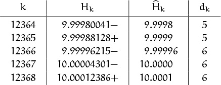
Estimate the total number of digits in the table, ![]() , with an absolute error of O(n).
, with an absolute error of O(n).
49. In Chapter 6 we considered the tale of a worm that reaches the end of a stretching band after n seconds, where Hn–1 < 100 ≤ Hn. Prove that if n is a positive integer such that Hn–1 ≤ α ≤ Hn, then
![]() eα –γ
eα –γ![]() ≤ n ≤
≤ n ≤ ![]() eα–γ
eα–γ![]() .
.
50. Venture capitalists in Silicon Valley are being offered a deal giving them a chance for an exponential payoff on their investments: For an n million dollar investment, where n ≥ 2, the GKP consortium promises to pay up to N million dollars after one year, where N = 10n. Of course there’s some risk; the actual deal is that GKP pays k million dollars with probability ![]() , for each integer k in the range 1 ≤ k ≤ N. (All payments are in megabucks, that is, in exact multiples of $1,000,000; the payoff is determined by a truly random process.) Notice that an investor always gets at least a million dollars back.
, for each integer k in the range 1 ≤ k ≤ N. (All payments are in megabucks, that is, in exact multiples of $1,000,000; the payoff is determined by a truly random process.) Notice that an investor always gets at least a million dollars back.
I once earned O(10–n) dollars.
a. What is the asymptotic expected return after one year, if n million dollars are invested? (In other words, what is the mean value of the payment?) Your answer should be correct within an absolute error of O(10–n) dollars.
b. What is the asymptotic probability that you make a profit, if you invest n million? (In other words, what is the chance that you get back more than you put in?) Your answer here should be correct within an absolute error of O(n–3).
Bonus problems
51. Prove or disprove: ![]() as n → ∞.
as n → ∞.
52. Show that there exists a power series A(z) = Σk≥0 anzn, convergent for all complex z, such that
53. Prove that if f(x) is a function whose derivatives satisfy
f′(x) ≤ 0 , –f″(x) ≤ 0 , f″′(x) ≤ 0, . . . , (–1)mf(m+1) (x) ≤ 0
for all x ≥ 0, then we have
In particular, the case f(x) = – ln(1 + x) proves (9.64) for all k, n > 0.
54. Let f(x) be a positive, differentiable function such that xf′(x) ≺ f(x) as x → ∞. Prove that
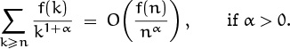
Hint: Consider the quantity ![]() .
.
55. Improve (9.99) to relative error O(n–3/2+5![]() ).
).
56. The quantity ![]() occurs in the analysis of many algorithms. Find its asymptotic value, with absolute error o(1).
occurs in the analysis of many algorithms. Find its asymptotic value, with absolute error o(1).
57. An asymptotic formula for Golomb’s sum Σk≥1 1/k![]() 1 + logn k
1 + logn k![]() 2 is derived in (9.54). Find an asymptotic formula for the analogous sum without floor brackets, Σk≥1 1/k(1 + logn k)2. Hint: Consider the integral
2 is derived in (9.54). Find an asymptotic formula for the analogous sum without floor brackets, Σk≥1 1/k(1 + logn k)2. Hint: Consider the integral ![]() .
.
58. Prove that
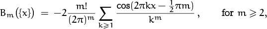
by using residue calculus, integrating
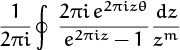
on the square contour z = x+iy, where ![]() , and letting the integer M tend to ∞
, and letting the integer M tend to ∞
59. Let Θn(t) = Σk e–(k+t)2/n, a periodic function of t. Show that the expansion of Θn(t) as a Fourier series is
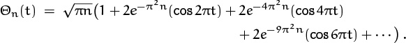
(This formula gives a rapidly convergent series for the sum Θn = Θn(0) in equation (9.93).)
60. Explain why the coefficients in the asymptotic expansion
all have denominators that are powers of 2.
61. Exercise 45 proves that the discrepancy D(α, n) is o(n) for all irrational numbers α. Exhibit an irrational α such that D(α, n) is not O(n1–![]() ) for any
) for any ![]() > 0.
> 0.
62. Given n, let ![]() be the largest entry in row n of Stirling’s subset triangle. Show that for all sufficiently large n, we have
be the largest entry in row n of Stirling’s subset triangle. Show that for all sufficiently large n, we have ![]() or
or ![]() , where
, where
Hint: This is difficult.
63. Prove that S. W. Golomb’s self-describing sequence of exercise 2.36 satisfies f(n) = ϕ2–ϕnϕ–1 + O(nϕ–1/log n).
64. Find a proof of the identity
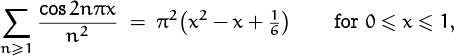
that uses only “Eulerian” (eighteenth-century) mathematics.
65. What are the coefficients of the asymptotic series
Research problems
66. Find a “combinatorial” proof of Stirling’s approximation. (Note that nn is the number of mappings of {1, 2, . . . , n} into itself, and n! is the number of mappings of {1, 2, . . . , n} onto itself.)
67. Consider an n × n array of dots, n ≥ 3, in which each dot has four neighbors. (At the edges we “wrap around” modulo n.) Let χn be the number of ways to assign the colors red, white, and blue to these dots in such a way that no neighboring dots have the same color. (Thus χ3 = 12.) Prove that
68. Let Qn be the least integer m such that Hm > n. Find the smallest integer n such that Qn ≠ ![]() en–γ +
en–γ + ![]()
![]() , or prove that no such n exist.
, or prove that no such n exist.
Th-th-th-that’s all, folks!