8. Discrete Probability

The element of chance enters into many of our attempts to understand the world we live in. A mathematical theory of probability allows us to calculate the likelihood of complex events if we assume that the events are governed by appropriate axioms. This theory has significant applications in all branches of science, and it has strong connections with the techniques we have studied in previous chapters.

Probabilities are called “discrete” if we can compute the probabilities of all events by summation instead of by integration. We are getting pretty good at sums, so it should come as no great surprise that we are ready to apply our knowledge to some interesting calculations of probabilities and averages.

8.1 Definitions

Probability theory starts with the idea of a probability space, which is a set Ω of all things that can happen in a given problem together with a rule that assigns a probability Pr(ω) to each elementary event ω Ω. The probability Pr(ω) must be a nonnegative real number, and the condition

must hold in every discrete probability space. Thus, each value Pr(ω) must lie in the interval [0 . . 1]. We speak of Pr as a probability distribution, because it distributes a total probability of 1 among the events ω.

(Readers unfamiliar with probability theory will, with high probability, benefit from a perusal of Feller’s classic introduction to the subject [120].)

Here’s an example: If we’re rolling a pair of dice, the set Ω of elementary events is , where

Never say die.

is the set of all six ways that a given die can land. Two rolls such as and are considered to be distinct; hence this probability space has a total of 6² = 36 elements.

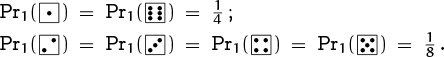
We usually assume that dice are “fair”—that each of the six possibilities for a particular die has probability , and that each of the 36 possible rolls in Ω has probability . But we can also consider “loaded” dice in which there is a different distribution of probabilities. For example, let

Careful: They might go off.

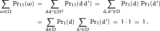
Then Σ_dDPr₁(d) = 1, so Pr₁ is a probability distribution on the set D, and we can assign probabilities to the elements of Ω = D² by the rule

For example, . This is a valid distribution because

We can also consider the case of one fair die and one loaded die,

in which case . Dice in the “real world” can’t really be expected to turn up equally often on each side, because they aren’t perfectly symmetrical; but is usually pretty close to the truth.

If all sides of a cube were identical, how could we tell which side is face up?

An event is a subset of Ω. In dice games, for example, the set

is the event that “doubles are thrown.” The individual elements ω of Ω are called elementary events because they cannot be decomposed into smaller subsets; we can think of ω as a one-element event {ω}.

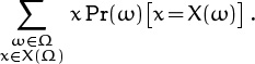
The probability of an event A is defined by the formula

and in general if R(ω) is any statement about ω, we write ‘Pr (R(ω))’ for the sum of all Pr(ω) such that R(ω) is true. Thus, for example, the probability of doubles with fair dice is ; but when both dice are loaded with probability distribution Pr₁ it is . Loading the dice makes the event “doubles are thrown” more probable.

(We have been using Σ-notation in a more general sense here than defined in Chapter 2: The sums in (8.1) and (8.4) occur over all elements ω of an arbitrary set, not over integers only. However, this new development is not really alarming; we can agree to use special notation under a Σ whenever nonintegers are intended, so there will be no confusion with our ordinary conventions. The other definitions in Chapter 2 are still valid; in particular, the definition of infinite sums in that chapter gives the appropriate interpretation to our sums when the set Ω is infinite. Each probability is nonnegative, and the sum of all probabilities is bounded, so the probability of event A in (8.4) is well defined for all subsets A ⊆ Ω.)

A random variable is a function defined on the elementary events ω of a probability space. For example, if Ω = D² we can define S(ω) to be the sum of the spots on the dice roll ω, so that = 6 + 3 = 9. The probability that the spots total seven is the probability of the event S(ω) = 7, namely

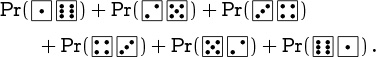
With fair dice (Pr = Pr₀₀), this happens with probability ; but with loaded dice (Pr = Pr₁₁), it happens with probability , the same as we observed for doubles.

It’s customary to drop the ‘(ω)’ when we talk about random variables, because there’s usually only one probability space involved when we’re working on any particular problem. Thus we say simply ‘S = 7’ for the event that a 7 was rolled, and ‘S = 4’ for the event .

A random variable can be characterized by the probability distribution of its values. Thus, for example, S takes on eleven possible values {2, 3, . . . , 12}, and we can tabulate the probability that S = s for each s in this set:

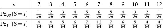
If we’re working on a problem that involves only the random variable S and no other properties of dice, we can compute the answer from these probabilities alone, without regard to the details of the set Ω = D². In fact, we could define the probability space to be the smaller set Ω = {2, 3, . . . , 12}, with whatever probability distribution Pr(s) is desired. Then ‘S = 4’ would be an elementary event. Thus we can often ignore the underlying probability space Ω and work directly with random variables and their distributions.

If two random variables X and Y are defined over the same probability space Ω, we can characterize their behavior without knowing everything about Ω if we know the “joint distribution”

Just Say No.

Pr(X = x and Y = y)

for each x in the range of X and each y in the range of Y. We say that X and Y are independent random variables if

for all x and y. Intuitively, this means that the value of X has no effect on the value of Y.

For example, if Ω is the set of dice rolls D², we can let S₁ be the number of spots on the first die and S₂ the number of spots on the second. Then the random variables S₁ and S₂ are independent with respect to each of the probability distributions Pr₀₀, Pr₁₁, and Pr₀₁ discussed earlier, because we defined the dice probability for each elementary event dd′ as a product of a probability for S₁ = d multiplied by a probability for S₂ = d′. We could have defined probabilities differently so that, say,

A dicey inequality.

but we didn’t do that, because different dice aren’t supposed to influence each other. With our definitions, both of these ratios are Pr(S₂ = 5)/ Pr(S₂ = 6).

We have defined S to be the sum of the two spot values, S₁ + S₂. Let’s consider another random variable P, the product S₁S₂. Are S and P independent? Informally, no; if we are told that S = 2, we know that P must be 1. Formally, no again, because the independence condition (8.5) fails spectacularly (at least in the case of fair dice): For all legal values of s and p, we have 0 < Pr₀₀(S = s) ̭ Pr₀₀(P = p) ; this can’t equal Pr₀₀(S = s and P = p), which is a multiple of .

If we want to understand the typical behavior of a given random variable, we often ask about its “average” value. But the notion of “average” is ambiguous; people generally speak about three different kinds of averages when a sequence of numbers is given:

• the mean (which is the sum of all values, divided by the number of values);

• the median (which is the middle value, numerically);

• the mode (which is the value that occurs most often).

For example, the mean of (3, 1, 4, 1, 5) is ; the median is 3; the mode is 1.

But probability theorists usually work with random variables instead of with sequences of numbers, so we want to define the notion of an “average” for random variables too. Suppose we repeat an experiment over and over again, making independent trials in such a way that each value of X occurs with a frequency approximately proportional to its probability. (For example, we might roll a pair of dice many times, observing the values of S and/or P.) We’d like to define the average value of a random variable so that such experiments will usually produce a sequence of numbers whose mean, median, or mode is approximately the same as the mean, median, or mode of X, according to our definitions.

Here’s how it can be done: The mean of a random real-valued variable X on a probability space Ω is defined to be

if this potentially infinite sum exists. (Here X(Ω) stands for the set of all real values x for which Pr(X = x) is nonzero.) The median of X is defined to be the set of all x X(Ω) such that

And the mode of X is defined to be the set of all x X(Ω) such that

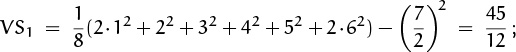
In our dice-throwing example, the mean of S turns out to be in distribution Pr₀₀, and it also turns out to be 7 in distribution Pr₁₁. The median and mode both turn out to be {7} as well, in both distributions. So S has the same average under all three definitions. On the other hand the P in distribution Pr₀₀ turns out to have a mean value of = 12.25; its median is {10}, and its mode is {6, 12}. The mean of P is unchanged if we load the dice with distribution Pr₁₁, but the median drops to {8} and the mode becomes {6} alone.

Probability theorists have a special name and notation for the mean of a random variable: They call it the expected value, and write

In our dice-throwing example, this sum has 36 terms (one for each element of Ω), while (8.6) is a sum of only eleven terms. But both sums have the same value, because they’re both equal to

The mean of a random variable turns out to be more meaningful in applications than the other kinds of averages, so we shall largely forget about medians and modes from now on. We will use the terms “expected value,” “mean,” and “average” almost interchangeably in the rest of this chapter.

I get it: On average, “average” means “mean.”

If X and Y are any two random variables defined on the same probability space, then X + Y is also a random variable on that space. By formula (8.9), the average of their sum is the sum of their averages:

Similarly, if α is any constant we have the simple rule

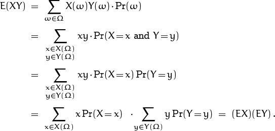
But the corresponding rule for multiplication of random variables is more complicated in general; the expected value is defined as a sum over elementary events, and sums of products don’t often have a simple form. In spite of this difficulty, there is a very nice formula for the mean of a product in the special case that the random variables are independent:

We can prove this by the distributive law for products,

For example, we know that S = S₁ + S₂ and P = S₁S₂, when S₁ and S₂ are the numbers of spots on the first and second of a pair of fair dice. We have ES₁ = ES₂ = , hence ES = 7; furthermore S₁ and S₂ are independent, so , as claimed earlier. We also have E(S+P) = ES+EP = 7+ . But S and P are not independent, so we cannot assert that . In fact, the expected value of SP turns out to equal in distribution Pr₀₀, while it equals 112 (exactly) in distribution Pr₁₁.

8.2 Mean and Variance

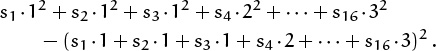
The next most important property of a random variable, after we know its expected value, is its variance, defined as the mean square deviation from the mean:

If we denote EX by μ, the variance VX is the expected value of (X – μ)². This measures the “spread” of X’s distribution.

As a simple example of variance computation, let’s suppose we have just been made an offer we can’t refuse: Someone has given us two gift certificates for a certain lottery. The lottery organizers sell 100 tickets for each weekly drawing. One of these tickets is selected by a uniformly random process—that is, each ticket is equally likely to be chosen—and the lucky ticket holder wins a hundred million dollars. The other 99 ticket holders win nothing.

(Slightly subtle point: There are two probability spaces, depending on what strategy we use; but EX₁ and EX₂ are the same in both.)

We can use our gift in two ways: Either we buy two tickets in the same lottery, or we buy one ticket in each of two lotteries. Which is a better strategy? Let’s try to analyze this by letting X₁ and X₂ be random variables that represent the amount we win on our first and second ticket. The expected value of X₁, in millions, is

and the same holds for X₂. Expected values are additive, so our average total winnings will be

E(X₁ + X₂) = EX₁ + EX₂ = 2 million dollars,

regardless of which strategy we adopt.

Still, the two strategies seem different. Let’s look beyond expected values and study the exact probability distribution of X₁ + X₂:

If we buy two tickets in the same lottery we have a 98% chance of winning nothing and a 2% chance of winning $100 million. If we buy them in different lotteries we have a 98.01% chance of winning nothing, so this is slightly more likely than before; and we have a 0.01% chance of winning $200 million, also slightly more likely than before; and our chances of winning $100 million are now 1.98%. So the distribution of X₁ + X₂ in this second situation is slightly more spread out; the middle value, $100 million, is slightly less likely, but the extreme values are slightly more likely.

It’s this notion of the spread of a random variable that the variance is intended to capture. We measure the spread in terms of the squared deviation of the random variable from its mean. In case 1, the variance is therefore

.98(0M – 2M)² + .02(100M – 2M)² = 196M²;

in case 2 it is

.9801(0M – 2M)² + .0198(100M – 2M)² + .0001(200M – 2M)² = 198M².

As we expected, the latter variance is slightly larger, because the distribution of case 2 is slightly more spread out.

When we work with variances, everything is squared, so the numbers can get pretty big. (The factor M² is one trillion, which is somewhat imposing even for high-stakes gamblers.) To convert the numbers back to the more meaningful original scale, we often take the square root of the variance. The resulting number is called the standard deviation, and it is usually denoted by the Greek letter σ:

Interesting: The variance of a dollar amount is expressed in units of square dollars.

The standard deviations of the random variables X₁ + X₂ in our two lottery strategies are = 14.00M and ≈ 14.071247M. In some sense the second alternative is about $71,247 riskier.

How does the variance help us choose a strategy? It’s not clear. The strategy with higher variance is a little riskier; but do we get the most for our money by taking more risks or by playing it safe? Suppose we had the chance to buy 100 tickets instead of only two. Then we could have a guaranteed victory in a single lottery (and the variance would be zero); or we could gamble on a hundred different lotteries, with a .99¹⁰⁰ ≈ .366 chance of winning nothing but also with a nonzero probability of winning up to $10,000,000,000. To decide between these alternatives is beyond the scope of this book; all we can do here is explain how to do the calculations.

Another way to reduce risk might be to bribe the lottery officials. I guess that’s where probability becomes indiscreet.

(N.B.: Opinions expressed in these margins do not necessarily represent the opinions of the management.)

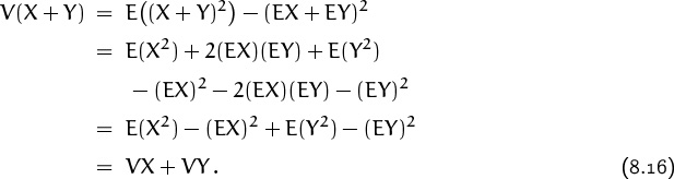
In fact, there is a simpler way to calculate the variance, instead of using the definition (8.13). (We suspect that there must be something going on in the mathematics behind the scenes, because the variances in the lottery example magically came out to be integer multiples of M².) We have

E([X – EX]2)	=	E(X2 – 2X[EX] + [EX]2)
	=	E(X2 – 2X[EX][EX] + [EX]2,

since (EX) is a constant; hence

“The variance is the mean of the square minus the square of the mean.”

For example, the mean of (X₁ + X₂)² comes to .98(0M)² + .02(100M)² = 200M² or to .9801(0M)² + .0198(100M)² + .0001(200M)² = 202M² in the lottery problem. Subtracting 4M² (the square of the mean) gives the results we obtained the hard way.

There’s an even easier formula yet, if we want to calculate V(X+Y) when X and Y are independent: We have

E([X + Y]2)	=	E(X2 + 2XY + Y2)
	=	E[X2] + 2[EX][EY] + E[Y2],

since we know that E(XY) = (EX)(EY) in the independent case. Therefore

“The variance of a sum of independent random variables is the sum of their variances.” For example, the variance of the amount we can win with a single lottery ticket is

– [EX₁]² = .99[OM]² + .01[100M]² – [1M]² = 99M².

Therefore the variance of the total winnings of two lottery tickets in two separate (independent) lotteries is 2×99M² = 198M². And the corresponding variance for n independent lottery tickets is n × 99M².

The variance of the dice-roll sum S drops out of this same formula, since S = S₁ + S₂ is the sum of two independent random variables. We have

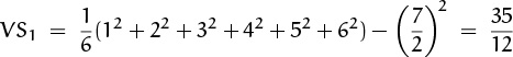
when the dice are fair; hence . The loaded die has

hence VS = = 7.5 when both dice are loaded. Notice that the loaded dice give S a larger variance, although S actually assumes its average value 7 more often than it would with fair dice. If our goal is to shoot lots of lucky 7’s, the variance is not our best indicator of success.

OK, we have learned how to compute variances. But we haven’t really seen a good reason why the variance is a natural thing to compute. Everybody does it, but why? The main reason is Chebyshev’s inequality ([29] and [57]), which states that the variance has a significant property:

If he proved it in 1867, it’s a classic ’67 Chebyshev.

(This is different from the monotonic inequalities of Chebyshev that we encountered in Chapter 2.) Very roughly, (8.17) tells us that a random variable X will rarely be far from its mean EX if its variance VX is small. The proof is amazingly simple. We have

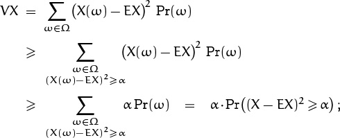
dividing by α finishes the proof.

If we write μ for the mean and σ for the standard deviation, and if we replace α by c²VX in (8.17), the condition (X – EX)² ≥ c²VX is the same as (X – μ)² ≥ (cσ)²; hence (8.17) says that

Thus, X will lie within c standard deviations of its mean value except with probability at most 1/c². A random variable will lie within 2σ of μ at least 75% of the time; it will lie between μ – 10σ and μ + 10σ at least 99% of the time. These are the cases α = 4VX and α = 100VX of Chebyshev’s inequality.

If we roll a pair of fair dice n times, the total value of the n rolls will almost always be near 7n, for large n. Here’s why: The variance of n independent rolls is n. A variance of n means a standard deviation of only

So Chebyshev’s inequality tells us that the final sum will lie between

in at least 99% of all experiments when n fair dice are rolled. For example, the odds are better than 99 to 1 that the total value of a million rolls will be between 6.975 million and 7.025 million.

In general, let X be any random variable over a probability space Ω, having finite mean μ and finite standard deviation σ. Then we can consider the probability space Ωⁿ whose elementary events are n-tuples (ω₁, ω₂, . . . , ω_n) with each ω_k Ω, and whose probabilities are

Pr(ω₁, ω₂, . . . , ω_n) = Pr(ω₁) Pr(ω₂) . . . Pr(ω_n) .

If we now define random variables X_k by the formula

X_k(ω₁, ω₂, . . . , ω_n) = X(ω_k) ,

the quantity

X₁ + X₂ + · · · + X_n

is a sum of n independent random variables, which corresponds to taking n independent “samples” of X on Ω and adding them together. The mean of X₁ + X₂ + · · · + X_n is nμ, and the standard deviation is σ; hence the average of the n samples,

[X1 + X2 + ... + X_n),

will lie between μ – 10σ/ and μ + 10σ/ at least 99% of the time. In other words, if we choose a large enough value of n, the average of n independent samples will almost always be very near the expected value EX. (An even stronger theorem called the Strong Law of Large Numbers is proved in textbooks of probability theory; but the simple consequence of Chebyshev’s inequality that we have just derived is enough for our purposes.)

(That is, the average will fall between the stated limits in at least 99% of all cases when we look at a set of n independent samples, for any fixed value of n. Don’t misunderstand this as a statement about the averages of an infinite sequence X₁, X₂ , X₃, . . . as n varies.)

Sometimes we don’t know the characteristics of a probability space, and we want to estimate the mean of a random variable X by sampling its value repeatedly. (For example, we might want to know the average temperature at noon on a January day in San Francisco; or we may wish to know the mean life expectancy of insurance agents.) If we have obtained independent empirical observations X₁, X₂, . . . , X_n, we can guess that the true mean is approximately

And we can also make an estimate of the variance, using the formula

The (n–1)’s in this formula look like typographic errors; it seems they should be n’s, as in (8.19), because the true variance VX is defined by expected values in (8.15). Yet we get a better estimate with n – 1 instead of n here, because definition (8.20) implies that

Here’s why:

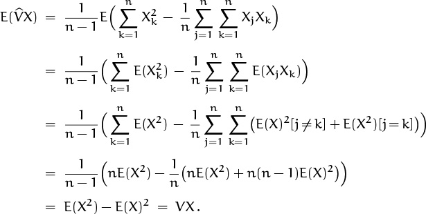
(This derivation uses the independence of the observations when it replaces E(X_jX_k) by (EX)²[j ≠ k] + E(X²)[j = k].)

In practice, experimental results about a random variable X are usually obtained by calculating a sample mean = ÊX and a sample standard deviation , and presenting the answer in the form . For example, here are ten rolls of two supposedly fair dice:

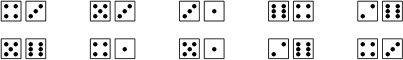
The sample mean of the spot sum S is

= (7 + 11 + 8 + 5 + 4 + 6 + 10 + 8 + 8 + 7)/10 = 7.4;

the sample variance is

(7² + 11² + 8² + 5² + 4² + 6² + 10² + 8² + 8² + 7² – 10²)/9 ≈ 2.1² .

We estimate the average spot sum of these dice to be 7.4±2.1/ ≈ 7.4±0.7, on the basis of these experiments.

Let’s work one more example of means and variances, in order to show how they can be calculated theoretically instead of empirically. One of the questions we considered in Chapter 5 was the “football victory problem,” where n hats are thrown into the air and the result is a random permutation of hats. We showed in equation (5.51) that there’s a probability of n¡/n! ≈ 1/e that nobody gets the right hat back. We also derived the formula

for the probability that exactly k people end up with their own hats.

Restating these results in the formalism just learned, we can consider the probability space Π_n of all n! permutations π of {1, 2, . . . , n}, where Pr(π) = 1/n! for all π Π_n. The random variable

F_n(π) = number of “fixed points” of π ,    for π Π_n,

measures the number of correct hat-falls in the football victory problem. Equation (8.22) gives Pr(F_n = k), but let’s pretend that we don’t know any such formula; we merely want to study the average value of F_n, and its standard deviation.

Not to be confused with a Fibonacci number.

The average value is, in fact, extremely easy to calculate, avoiding all the complexities of Chapter 5. We simply observe that

Fn[π]	=	Fn, 1[π] + Fn,2[π] + ... + Fn,n[π],
Fn,k[π]	=	[position k of π is a fixed point],	for π Πn.

Hence

EF_n = EF_n,1 + EF_n,2 + · · · + EF_n,n .

And the expected value of F_n,k is simply the probability that F_n,k = 1, which is 1/n because exactly (n – 1)! of the n! permutations π = π₁π₂ . . . π_n Π_n have π_k = k. Therefore

On the average, one hat will be in its correct place. “A random permutation has one fixed point, on the average.”

One the average.

Now what’s the standard deviation? This question is more difficult, because the F_n,k’s are not independent of each other. But we can calculate the variance by analyzing the mutual dependencies among them:

(We used a similar trick when we derived (2.33) in Chapter 2.) Now _,k = F_n,k, since F_n,k is either 0 or 1; hence E(,_k) = EF_n,k = 1/n as before. And if j < k we have E(F_n,j F_n,k) = Pr(π has both j and k as fixed points) = (n – 2)!/n! = 1/n(n – 1). Therefore

(As a check when n = 3, we have ) The variance is E() – (EF_n)² = 1, so the standard deviation (like the mean) is 1. “A random permutation of n ≥ 2 elements has 1 ± 1 fixed points.”

8.3 Probability Generating Functions

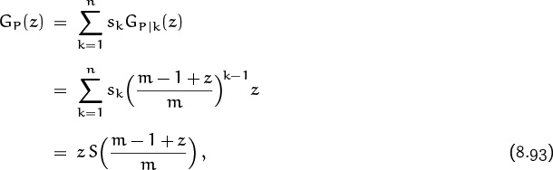
If X is a random variable that takes only nonnegative integer values, we can capture its probability distribution nicely by using the techniques of Chapter 7. The probability generating function or pgf of X is

This power series in z contains all the information about the random variable X. We can also express it in two other ways:

The coefficients of G_X(z) are nonnegative, and they sum to 1; the latter condition can be written

Conversely, any power series G(z) with nonnegative coefficients and with G(1) = 1 is the pgf of some random variable.

The nicest thing about pgf’s is that they usually simplify the computation of means and variances. For example, the mean is easily expressed:

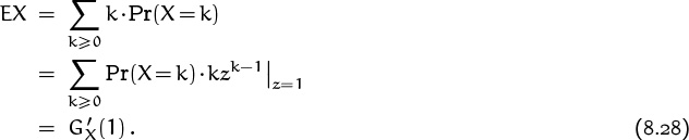
We simply differentiate the pgf with respect to z and set z = 1.

The variance is only slightly more complicated:

Therefore

Equations (8.28) and (8.29) tell us that we can compute the mean and variance if we can compute the values of two derivatives, and . We don’t have to know a closed form for the probabilities; we don’t even have to know a closed form for G_X(z) itself.

It is convenient to write

when G is any function, since we frequently want to compute these combinations of derivatives.

The second-nicest thing about pgf’s is that they are comparatively simple functions of z, in many important cases. For example, let’s look at the uniform distribution of order n, in which the random variable takes on each of the values {0, 1, . . . , n – 1} with probability 1/n. The pgf in this case is

We have a closed form for U_n(z) because this is a geometric series.

But this closed form proves to be somewhat embarrassing: When we plug in z = 1 (the value of z that’s most critical for the pgf), we get the undefined ratio 0/0, even though U_n(z) is a polynomial that is perfectly well defined at any value of z. The value U_n(1) = 1 is obvious from the non-closed form (1 + z + · · · + z^n–1)/n, yet it seems that we must resort to L’Hospital’s rule to find lim_z→1 U_n(z) if we want to determine U_n(1) from the closed form. The determination of by L’Hospital’s rule will be even harder, because there will be a factor of (z–1)² in the denominator; will be harder still.

Luckily there’s a nice way out of this dilemma. If G(z) = Σ_n≥0 g_nzⁿ is any power series that converges for at least one value of z with |z| > 1, the power series G′(z) = Σ_n≥0 g_nz^n–1 will also have this property, and so will G″(z), G″′(z), etc. Therefore by Taylor’s theorem we can write

all derivatives of G(z) at z = 1 will appear as coefficients, when G(1 + t) is expanded in powers of t.

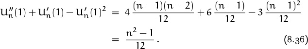
For example, the derivatives of the uniform pgf U_n(z) are easily found in this way:

Comparing this to (8.33) gives

and in general (1) = (n – 1)^m/(m + 1), although we need only the cases m = 1 and m = 2 to compute the mean and the variance. The mean of the uniform distribution is

and the variance is

The third-nicest thing about pgf’s is that the product of pgf’s corresponds to the sum of independent random variables. We learned in Chapters 5 and 7 that the product of generating functions corresponds to the convolution of sequences; but it’s even more important in applications to know that the convolution of probabilities corresponds to the sum of independent random variables. Indeed, if X and Y are random variables that take on nothing but integer values, the probability that X + Y = n is

If X and Y are independent, we now have

a convolution. Therefore—and this is the punch line —

Earlier this chapter we observed that V(X + Y) = VX + VY when X and Y are independent. Let F(z) and G(z) be the pgf’s for X and Y, and let H(z) be the pgf for X + Y. Then

H(z) = F(z)G(z) ,

and our formulas (8.28) through (8.31) for mean and variance tell us that we must have

These formulas, which are properties of the derivatives Mean(H) = H′(1) and Var(H) = H″(1) + H′(1) – H′(1)², aren’t valid for arbitrary function products H(z) = F(z)G(z); we have

H′[z]	=	F′[z]G[z] + F[z]G′[z],
H˝[z]	=	F˝[z]G[z] + 2F′[z]G′[z] + F[z] G˝ [z].

But if we set z = 1, we can see that (8.38) and (8.39) will be valid in general provided only that

and that the derivatives exist. The “probabilities” don’t have to be in [0 . . 1] for these formulas to hold. We can normalize the functions F(z) and G(z) by dividing through by F(1) and G(1) in order to make this condition valid, whenever F(1) and G(1) are nonzero.

I’ll graduate magna cum ulant.

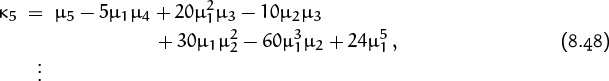
Mean and variance aren’t the whole story. They are merely two of an infinite series of so-called cumulant statistics introduced by the Danish astronomer Thorvald Nicolai Thiele [351] in 1903. The first two cumulants κ₁ and κ₂ of a random variable are what we have called the mean and the variance; there also are higher-order cumulants that express more subtle properties of a distribution. The general formula

defines the cumulants of all orders, when G(z) is the pgf of a random variable.

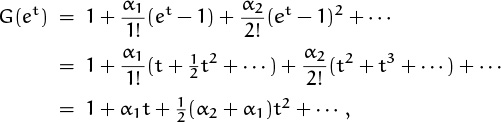
Let’s look at cumulants more closely. If G(z) is the pgf for X, we have

where

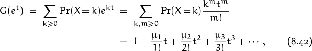
This quantity μ_m is called the “mth moment” of X. We can take exponentials on both sides of (8.41), obtaining another formula for G(e^t):

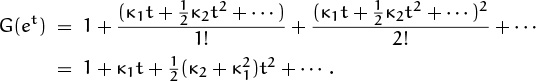
Equating coefficients of powers of t leads to a series of formulas

defining the cumulants in terms of the moments. Notice that κ₂ is indeed the variance, E(X²) – (EX)², as claimed.

Equation (8.41) makes it clear that the cumulants defined by the product F(z)G(z) of two pgf’s will be the sums of the corresponding cumulants of F(z) and G(z), because logarithms of products are sums. Therefore all cumulants of the sum of independent random variables are additive, just as the mean and variance are. This property makes cumulants more important than moments.

“For these higher half-invariants we shall propose no special names.”
    —T. N. Thiele [351]

If we take a slightly different tack, writing

equation (8.33) tells us that the α’s are the “factorial moments”

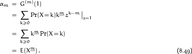
It follows that

and we can express the cumulants in terms of the derivatives G^(m)(1):

This sequence of formulas yields “additive” identities that extend (8.38) and (8.39) to all the cumulants.

Let’s get back down to earth and apply these ideas to simple examples. The simplest case of a random variable is a “random constant,” where X has a certain fixed value x with probability 1. In this case G_X(z) = z^x, and ln G_X(e^t) = xt; hence the mean is x and all other cumulants are zero. It follows that the operation of multiplying any pgf by z^x increases the mean by x but leaves the variance and all other cumulants unchanged.

How do probability generating functions apply to dice? The distribution of spots on one fair die has the pgf

where U₆ is the pgf for the uniform distribution of order 6. The factor ‘z’ adds 1 to the mean, so the mean is 3.5 instead of = 2.5 as given in (8.35); but an extra ‘z’ does not affect the variance (8.36), which equals .

The pgf for total spots on two independent dice is the square of the pgf for spots on one die,

Gs[z]	=
	=	z2U6[z]2.

If we roll a pair of fair dice n times, the probability that we get a total of k spots overall is, similarly,

[zK] Gs (z)n	=	[zk] z2n U6 (z)2n
	=	[zk–2n] U6 (z)2n.

Hat distribution is a different kind of uniform distribution.

In the hats-off-to-football-victory problem considered earlier, otherwise known as the problem of enumerating the fixed points of a random permutation, we know from (5.49) that the pgf is

Therefore

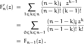
Without knowing the details of the coefficients, we can conclude from this recurrence = F_n–1[z] that [z] = F_n–m [z]; hence

This formula makes it easy to calculate the mean and variance; we find as before (but more quickly) that they are both equal to 1 when n ≥ 2.

In fact, we can now show that the mth cumulant κ_m of this random variable is equal to 1 whenever n ≥ m. For the mth cumulant depends only on , and these are all equal to 1; hence we obtain the same answer for the mth cumulant as we do when we replace F_n(z) by the limiting pgf

which has (1) = 1 for derivatives of all orders. The cumulants of F_∞ are identically equal to 1, because

8.4 Flipping Coins

Now let’s turn to processes that have just two outcomes. If we flip a coin, there’s probability p that it comes up heads and probability q that it comes up tails, where

p + q = 1 .

(We assume that the coin doesn’t come to rest on its edge, or fall into a hole, etc.) Throughout this section, the numbers p and q will always sum to 1. If the coin is fair, we have p = q = ; otherwise the coin is said to be biased.

Con artists know that p ≈ 0.1 when you spin a newly minted U.S. penny on a smooth table. (The weight distribution makes Lincoln’s head fall downward.)

The probability generating function for the number of heads after one toss of a coin is

If we toss the coin n times, always assuming that different coin tosses are independent, the number of heads is generated by

according to the binomial theorem. Thus, the chance that we obtain exactly k heads in n tosses is p^k q^n–k. This sequence of probabilities is called the binomial distribution.

Suppose we toss a coin repeatedly until heads first turns up. What is the probability that exactly k tosses will be required? We have k = 1 with probability p (since this is the probability of heads on the first flip); we have k = 2 with probability qp (since this is the probability of tails first, then heads); and for general k the probability is q^k–1p. So the generating function is

Repeating the process until n heads are obtained gives the pgf

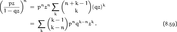
This, incidentally, is zⁿ times

the generating function for the negative binomial distribution.

The probability space in example (8.59), where we flip a coin until n heads have appeared, is different from the probability spaces we’ve seen earlier in this chapter, because it contains infinitely many elements. Each element is a finite sequence of heads and/or tails, containing precisely n heads in all, and ending with heads; the probability of such a sequence is pⁿq^k–n, where k – n is the number of tails. Thus, for example, if n = 3 and if we write H for heads and T for tails, the sequence THTTTHH is an element of the probability space, and its probability is qpqqqpp = p³q⁴.

Heads I win, tails you lose.
No? OK; tails you lose, heads I win.
No? Well, then, heads you lose, tails I win.

Let X be a random variable with the binomial distribution (8.57), and let Y be a random variable with the negative binomial distribution (8.60). These distributions depend on n and p. The mean of X is nH′(1) = np, since its pgf is H(z)ⁿ; the variance is

Thus the standard deviation is : If we toss a coin n times, we expect to get heads about np ± times. The mean and variance of Y can be found in a similar way: If we let

we have

hence G′(1) = pq/p² = q/p and G″(1) = 2pq²/p³ = 2q²/p². It follows that the mean of Y is nq/p and the variance is nq/p².

A simpler way to derive the mean and variance of Y is to use the reciprocal generating function

and to write

This polynomial F(z) is not a probability generating function, because it has a negative coefficient. But it does satisfy the crucial condition F(1) = 1. Thus F(z) is formally a binomial that corresponds to a coin for which we get heads with “probability” equal to –q/p; and G(z) is formally equivalent to flipping such a coin –1 times(!). The negative binomial distribution with parameters (n, p) can therefore be regarded as the ordinary binomial distribution with parameters (n′, p′) = (–n, –q/p). Proceeding formally, the mean must be n′p′ = (–n)(–q/p) = nq/p, and the variance must be n′p′q′ = (–n)(–q/p)(1 + q/p) = nq/p². This formal derivation involving negative probabilities is valid, because our derivation for ordinary binomials was based on identities between formal power series in which the assumption 0 ≤ p ≤ 1 was never used.

The probability is negative that I’m getting younger.

Oh? Then it’s > 1 that you’re getting older, or staying the same.

Let’s move on to another example: How many times do we have to flip a coin until we get heads twice in a row? The probability space now consists of all sequences of H’s and T’s that end with HH but have no consecutive H’s until the final position:

Ω = {HH, THH, TTHH, HTHH, TTTHH, THTHH, HTTHH, . . . } .

The probability of any given sequence is obtained by replacing H by p and T by q; for example, the sequence THTHH will occur with probability

Pr(THTHH) = qpqpp = p³q² .

We can now play with generating functions as we did at the beginning of Chapter 7, letting S be the infinite sum

S = HH + THH + TTHH + HTHH + TTTHH + THTHH + HTTHH + · · ·

of all the elements of Ω. If we replace each H by pz and each T by qz, we get the probability generating function for the number of flips needed until two consecutive heads turn up.

There’s a curious relation between S and the sum of domino tilings

in equation (7.1). Indeed, we obtain S from T if we replace each by T and each by HT, then tack on an HH at the end. This correspondence is easy to prove because each element of Ω has the form (T + HT)ⁿHH for some n ≥ 0, and each term of T has the form . Therefore by (7.4) we have

S = (1 – T – HT)^–1HH ,

and the probability generating function for our problem is

Our experience with the negative binomial distribution gives us a clue that we can most easily calculate the mean and variance of (8.64) by writing

G[z]

=

where

F[z]

=

and by calculating the “mean” and “variance” of this pseudo-pgf F(z). (Once again we’ve introduced a function with F(1) = 1.) We have

F′[1]	=	[–q – 2pq]/p2 = 2 – p–1 –p–2 ;
F˝[1]	=	–2pq/p2 = 2 – 2p–1.

Therefore, since z² = F(z)G(z), Mean(z²) = 2, and Var(z²) = 0, the mean and variance of distribution G(z) are

When p = the mean and variance are 6 and 22, respectively. (Exercise 4 discusses the calculation of means and variances by subtraction.)

Now let’s try a more intricate experiment: We will flip coins until the pattern THTTH is first obtained. The sum of winning positions is now

S	=	THTTH + HTHTTH + TTHTTH
		+ HHTHTTH + HTTHTTH + THTHTTH + TTTHTTH + · · · ;

this sum is more difficult to describe than the previous one. If we go back to the method by which we solved the domino problems in Chapter 7, we can obtain a formula for S by considering it as a “finite state language” defined by the following “automaton”:

“‘You really are an automaton—a calculating machine,’ I cried. ‘There is something positively inhuman in you at times.’”
    —J. H. Watson [83]

The elementary events in the probability space are the sequences of H’s and T’s that lead from state 0 to state 5. Suppose, for example, that we have just seen THT; then we are in state 3. Flipping tails now takes us to state 4; flipping heads in state 3 would take us to state 2 (not all the way back to state 0, since the TH we’ve just seen may be followed by TTH).

In this formulation, we can let S_k be the sum of all sequences of H’s and T’s that lead to state k; it follows that

S0	=	1 + S0 H + S2 H,
S1	=	S0 T + S1 T + S4 T,
S2	=	S1 H + S3 H,
S3	=	S2 T,
S4	=	S3 T,
S5	=	S4 H,

Now the sum S in our problem is S₅; we can obtain it by solving these six equations in the six unknowns S₀, S₁, . . . , S₅. Replacing H by pz and T by qz gives generating functions where the coefficient of zⁿ in S_k is the probability that we are in state k after n flips.

In the same way, any diagram of transitions between states, where the transition from state j to state k occurs with given probability p_j,k, leads to a set of simultaneous linear equations whose solutions are generating functions for the state probabilities after n transitions have occurred. Systems of this kind are called Markov processes, and the theory of their behavior is intimately related to the theory of linear equations.

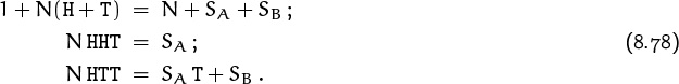
But the coin-flipping problem can be solved in a much simpler way, without the complexities of the general finite-state approach. Instead of six equations in six unknowns S₀, S₁, . . . , S₅, we can characterize S with only two equations in two unknowns. The trick is to consider the auxiliary sum N = S₀ + S₁ + S₂ + S₃ + S₄ of all flip sequences that don’t contain any occurrences of the given pattern THTTH:

N = 1 + H + T + HH + · · · + THTHT + THTTT + · · · .

We have

because every term on the left either ends with THTTH (and belongs to S) or doesn’t (and belongs to N); conversely, every term on the right is either empty or belongs to N H or N T. And we also have the important additional equation

because every term on the left completes a term of S after either the first H or the second H, and because every term on the right belongs to the left.

The solution to these two simultaneous equations is easily obtained: We have N = (1 – S)(1 – H – T)^–1 from (8.67), hence

(1 – S)(1 – T – H)^–1 THTTH = S(1 + TTH) .

As before, we get the probability generating function G(z) for the number of flips if we replace H by pz and T by qz. A bit of simplification occurs since p + q = 1, and we find

hence the solution is

Notice that G(1) = 1, if pq ≠ 0; we do eventually encounter the pattern THTTH, with probability 1, unless the coin is rigged so that it always comes up heads or always tails.

To get the mean and variance of the distribution (8.69), we invert G(z) as we did in the previous problem, writing G(z) = z⁵/F(z) where F is a polynomial:

The relevant derivatives are

F′(1)	=	5 – (1 + pq2)/p2q3,
F′(1)	=	20 – 6pq2/p2q3;

and if X is the number of flips we get

When , the mean and variance are 36 and 996.

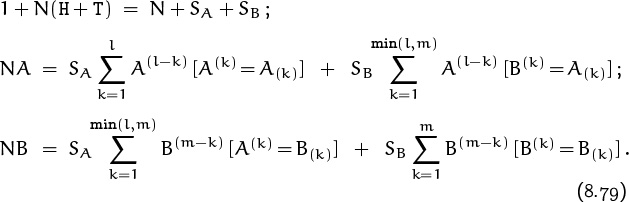
Let’s get general: The problem we have just solved was “random” enough to show us how to analyze the case that we are waiting for the first appearance of an arbitrary pattern A of heads and tails. Again we let S be the sum of all winning sequences of H’s and T’s, and we let N be the sum of all sequences that haven’t encountered the pattern A yet. Equation (8.67) will remain the same; equation (8.68) will become

where m is the length of A, and where A^(k) and A_(k) denote respectively the last k characters and the first k characters of A. For example, if A is the pattern THTTH we just studied, we have

A⁽¹⁾ = H , A⁽²⁾ = TH , A⁽³⁾ = TTH , A⁽⁴⁾ = HTTH;

A₍₁₎ = T , A₍₂₎ = TH , A₍₃₎ = THT , A₍₄₎ = THTT.

Since the only perfect match is A⁽²⁾ = A₍₂₎, equation (8.73) reduces to (8.68).

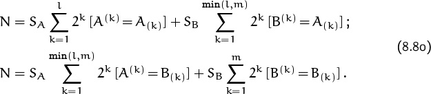
Let à be the result of substituting p^–1 for H and q^–1 for T in the pattern A. Then it is not difficult to generalize our derivation of (8.71) and (8.72) to conclude (exercise 20) that the general mean and variance are

In the special case we can interpret these formulas in a particularly simple way. Given a pattern A of m heads and tails, let

We can easily find the binary representation of this number by placing a ‘1’ under each position such that the string matches itself perfectly when it is superimposed on a copy of itself that has been shifted to start in this position:

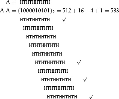
Equation (8.74) now tells us that the expected number of flips until pattern A appears is exactly 2(A:A), if we use a fair coin, because Ã_(k) = 2^k when p = q = . This result, first discovered by the Soviet mathematician A. D. Solov’ev in 1966 [331], seems paradoxical at first glance: Patterns with no self-overlaps occur sooner than overlapping patterns do! It takes almost twice as long to encounter HHHHH as it does to encounter HHHHT or THHHH.

“Chem bol’she periodov u nashego slova, tem pozzhe ono poıavlıaetsıa.”
    —A. D. Solov’ev

Now let’s consider an amusing game that was invented by (of all people) Walter Penney [289] in 1969. Alice and Bill flip a coin until either HHT or HTT occurs; Alice wins if the pattern HHT comes first, Bill wins if HTT comes first. This game—now called “Penney ante”—certainly seems to be fair, if played with a fair coin, because both patterns HHT and HTT have the same characteristics if we look at them in isolation: The probability generating function for the waiting time until HHT first occurs is

G(z) =

and the same is true for HTT. Therefore neither Alice nor Bill has an advantage, if they play solitaire.

Of course not! Who could they have an advantage over?

But there’s an interesting interplay between the patterns when both are considered simultaneously. Let S_A be the sum of Alice’s winning configurations, and let S_B be the sum of Bill’s:

S_A = HHT + HHHT + THHT + HHHHT + HTHHT + THHHT + ···;

S_B = HTT + THTT + HTHTT + TTHTT + THTHTT + TTTHTT + ···.

Also—taking our cue from the trick that worked when only one pattern was involved—let us denote by N the sum of all sequences in which neither player has won so far:

Then we can easily verify the following set of equations:

If we now set H = T = , the resulting value of S_A becomes the probability that Alice wins, and S_B becomes the probability that Bill wins. The three equations reduce to

and we find S_A = , S_B = . Alice will win about twice as often as Bill!

In a generalization of this game, Alice and Bill choose patterns A and B of heads and tails, and they flip coins until either A or B appears. The two patterns need not have the same length, but we assume that A doesn’t occur within B, nor does B occur within A. (Otherwise the game would be degenerate. For example, if A = HT and B = THTH, poor Bill could never win; and if A = HTH and B = TH, both players might claim victory simultaneously.) Then we can write three equations analogous to (8.73) and (8.78):

Here l is the length of A and m is the length of B. For example, if we have A = HTTHTHTH and B = THTHTTH, the two pattern-dependent equations are

N HTTHTHTH = S_A TTHTHTH + S_A + S_B TTHTHTH + S_B THTH;

  N THTHTTH = S_A THTTH + S_A TTH + S_B THTTH + S_B.

We obtain the victory probabilities by setting H = T = , if we assume that a fair coin is being used; this reduces the two crucial equations to

We can see what’s going on if we generalize the A:A operation of (8.76) to a function of two independent strings A and B:

Equations (8.80) now become simply

S_A(A:A) + S_B(B:A) = S_A(A:B) + S_B(B:B);

the odds in Alice’s favor are

(This beautiful formula was discovered by John Horton Conway [137].)

For example, if A = HTTHTHTH and B = THTHTTH as above, we have A:A = (10000001)₂ = 129, A:B = (0001010)₂ = 10, B:A = (0001001)₂ = 9, and B:B = (1000010)₂ = 66; so the ratio S_A/S_B is (66–9)/(129–10) = 57/119. Alice will win this one only 57 times out of every 176, on the average.

Strange things can happen in Penney’s game. For example, the pattern HHTH wins over the pattern HTHH with 3/2 odds, and HTHH wins over THHH with 7/5 odds. So HHTH ought to be much better than THHH. Yet THHH actually wins over HHTH, with 7/5 odds! The relation between patterns is not transitive. In fact, exercise 57 proves that if Alice chooses any pattern τ₁τ₂ . . . τ_l of length l ≥ 3, Bill can always ensure better than even chances of winning if he chooses the pattern ₂τ₁τ₂ . . . τ_l–1, where is the heads/tails opposite of τ₂.

Odd, odd.

8.5 Hashing

Let’s conclude this chapter by applying probability theory to computer programming. Several important algorithms for storing and retrieving information inside a computer are based on a technique called “hashing.” The general problem is to maintain a set of records that each contain a “key” value, K, and some data D(K) about that key; we want to be able to find D(K) quickly when K is given. For example, each key might be the name of a student, and the associated data might be that student’s homework grades.

“Somehow the verb ‘to hash’ magically became standard terminology for key transformation during the mid-1960s, yet nobody was rash enough to use such an undignified word publicly until 1967.”
    —D. E. Knuth [209]

In practice, computers don’t have enough capacity to set aside one memory cell for every possible key; billions of keys are possible, but comparatively few keys are actually present in any one application. One solution to the problem is to maintain two tables KEY[j] and DATA[j] for 1 ≤ j ≤ N, where N is the total number of records that can be accommodated; another variable n tells how many records are actually present. Then we can search for a given key K by going through the table sequentially in an obvious way:

S1 Set j := 1. (We’ve searched through all positions < j.)

S2 If j > n, stop. (The search was unsuccessful.)

S3 If KEY[j] = K, stop. (The search was successful.)

S4 Increase j by 1 and return to step S2. (We’ll try again.)

After a successful search, the desired data entry D(K) appears in DATA[j]. After an unsuccessful search, we can insert K and D(K) into the table by setting

n  :=  j,  KEY[n]  :=  K,  DATA[n]  :=  D(K),

assuming that the table was not already filled to capacity.

This method works, but it can be dreadfully slow; we need to repeat step S2 a total of n + 1 times whenever an unsuccessful search is made, and n can be quite large.

Hashing was invented to speed things up. The basic idea, in one of its popular forms, is to use m separate lists instead of one giant list. A “hash function” transforms every possible key K into a list number h(K) between 1 and m. An auxiliary table FIRST[i] for 1 ≤ i ≤ m points to the first record in list i; another auxiliary table NEXT[j] for 1 ≤ j ≤ N points to the record following record j in its list. We assume that

FIRST[i]	=	–1,	if list i is empty;
NEXT[j]	=	0 ,	if record j is the last in its list.

As before, there’s a variable n that tells how many records have been stored altogether.

For example, suppose the keys are names, and suppose that there are m = 4 lists based on the first letter of a name:

We start with four empty lists and with n = 0. If, say, the first record has Nora as its key, we have h(Nora) = 3, so Nora becomes the key of the first item in list 3. If the next two names are Glenn and Jim, they both go into list 2. Now the tables in memory look like this:

FIRST[1] = –1,  FIRST[2] = 2,  FIRST[3] = 1,  FIRST[4] = –1.

KEY[1]  =  Nora,     NEXT[1] = 0;

KEY[2]  =  Glenn,    NEXT[2] = 3;

KEY[3]  =  Jim,      NEXT[3] = 0 ;     n = 3.

(The values of DATA[1], DATA[2], and DATA[3] are confidential and will not be shown.) After 18 records have been inserted, the lists might contain the names

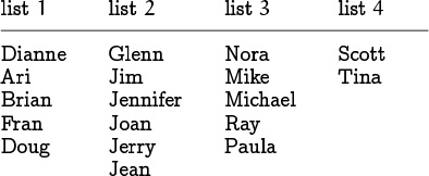
and these names would appear intermixed in the KEY array with NEXT entries to keep the lists effectively separate. If we now want to search for John, we have to scan through the six names in list 2 (which happens to be the longest list); but that’s not nearly as bad as looking at all 18 names.

Let’s hear it for the Concrete Math students who sat in the front rows and lent their names to this experiment.

Here’s a precise specification of the algorithm that searches for key K in accordance with this scheme:

H1 Set i := h(K) and j := FIRST[i].

H2 If j ≤ 0, stop. (The search was unsuccessful.)

H3 If KEY[j] = K, stop. (The search was successful.)

H4 Set i := j, then set j := NEXT[i] and return to step H2. (We’ll try again.)

For example, to search for Jennifer in the example given, step H1 would set i := 2 and j := 2; step H3 would find that Glenn ≠ Jennifer; step H4 would set j := 3; and step H3 would find Jim ≠ Jennifer. One more iteration of steps H4 and H3 would locate Jennifer in the table.

I bet their parents are glad about that.

After a successful search, the desired data D(K) appears in DATA[j], as in the previous algorithm. After an unsuccessful search, we can enter K and D(K) in the table by doing the following operations:

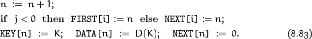
Now the table will once again be up to date.

We hope to get lists of roughly equal length, because this will make the task of searching about m times faster. The value of m is usually much greater than 4, so a factor of 1/m will be a significant improvement.

We don’t know in advance what keys will be present, but it is generally possible to choose the hash function h so that we can consider h(K) to be a random variable that is uniformly distributed between 1 and m, independent of the hash values of other keys that are present. In such cases computing the hash function is like rolling a die that has m faces. There’s a chance that all the records will fall into the same list, just as there’s a chance that a die will always turn up ; but probability theory tells us that the lists will almost always be pretty evenly balanced.

Analysis of Hashing: Introduction.

“Algorithmic analysis” is a branch of computer science that derives quantitative information about the efficiency of computer methods. “Probabilistic analysis of an algorithm” is the study of an algorithm’s running time, considered as a random variable that depends on assumed characteristics of the input data. Hashing is an especially good candidate for probabilistic analysis, because it is an extremely efficient method on the average, even though its worst case is too horrible to contemplate. (The worst case occurs when all keys have the same hash value.) Indeed, a computer programmer who uses hashing had better be a believer in probability theory.

Let P be the number of times step H3 is performed when the algorithm above is used to carry out a search. (Each execution of H3 is called a “probe” in the table.) If we know P, we know how often each step is performed, depending on whether the search is successful or unsuccessful:

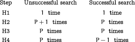
Thus the main quantity that governs the running time of the search procedure is the number of probes, P.

We can get a good mental picture of the algorithm by imagining that we are keeping an address book that is organized in a special way, with room for only one entry per page. On the cover of the book we note down the page number for the first entry in each of m lists; each name K determines the list h(K) that it belongs to. Every page inside the book refers to the successor page in its list. The number of probes needed to find an address in such a book is the number of pages we must consult.

If n items have been inserted, their positions in the table depend only on their respective hash values, h₁, h₂, . . . , h_n. Each of the mⁿ possible sequences h₁, h₂, . . . , h_n is considered to be equally likely, and P is a random variable depending on such a sequence.

Case 1: The key is not present.

Let’s consider first the behavior of P in an unsuccessful search, assuming that n records have previously been inserted into the hash table. In this case the relevant probability space consists of mⁿ⁺¹ elementary events

ω = (h₁, h₂, . . . , h_n, h_n+1)

where h_j is the hash value of the jth key inserted, and where h_n+1 is the hash value of the key for which the search is unsuccessful. We assume that the hash function h has been chosen properly so that Pr(ω) = 1/mⁿ⁺¹ for every such ω.

Check under the doormat.

For example, if m = n = 2, there are eight equally likely possibilities:

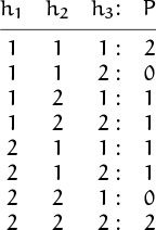
If h₁ = h₂ = h₃ we make two unsuccessful probes before concluding that the new key K is not present; if h₁ = h₂ ≠ h₃ we make none; and so on. This list of all possibilities shows that P has a probability distribution given by the pgf , when m = n = 2.

An unsuccessful search makes one probe for every item in list number h_n+1, so we have the general formula

The probability that h_j = h_n+1 is 1/m, for 1 ≤ j ≤ n; so it follows that

EP = E[h1 = h_n+1] + E[h₂ =h_n+1] + ... + E[h_n =h_n+1] =

Maybe we should do that more slowly: Let X_j be the random variable

X_j = X_j(ω) = [h_j = h_n+1].

Then P = X₁ + ··· + X_n, and EX_j = 1/m for all j ≤ n; hence

EP = EX₁ + ··· + EX_n = n/m.

Good: As we had hoped, the average number of probes is 1/m times what it was without hashing. Furthermore the random variables X_j are independent, and they each have the same probability generating function

Xj(z)

=

therefore the pgf for the total number of probes in an unsuccessful search is

This is a binomial distribution, with p = 1/m and q = (m – 1)/m; in other words, the number of probes in an unsuccessful search behaves just like the number of heads when we toss a biased coin whose probability of heads is 1/m on each toss. Equation (8.61) tells us that the variance of P is therefore

When m is large, the variance of P is approximately n/m, so the standard deviation is approximately .

Case 2: The key is present.

Now let’s look at successful searches. In this case the appropriate probability space is a bit more complicated, depending on our application: We will let Ω be the set of all elementary events

where h_j is the hash value for the jth key as before, and where k is the index of the key being sought (the key whose hash value is h_k). Thus we have 1 ≤ h_j ≤ m for 1 ≤ j ≤ n, and 1 ≤ k ≤ n; there are mⁿ · n elementary events ω in all.

Let s_j be the probability that we are searching for the jth key that was inserted into the table. Then

if ω is the event (8.86). (Some applications search most often for the items that were inserted first, or for the items that were inserted last, so we will not assume that each s_j = 1/n.) Notice that ∑_ωΩ Pr(ω) = s_k = 1, hence (8.87) defines a legal probability distribution.

The number P of probes in a successful search is p if key K was the pth key to be inserted into its list. Therefore

or, if we let X_j be the random variable [h_j = h_k], we have

Suppose, for example, that we have m = 10 and n = 16, and that the hash values have the following “random” pattern:

(h₁, . . . , h₁₆) = 3 1 4 1 5 9 2 6 5 3 5 8 9 7 9 3;

(P₁, . . . , P₁₆) = 1 1 1 2 1 1 1 1 2 2 3 1 2 1 3 3.

Where have I seen that pattern before?

The number of probes needed to find the jth key is shown below h_j.

Equation (8.89) represents P as a sum of random variables, but we can’t simply calculate EP as EX₁+· · ·+EX_k because the quantity k itself is a random variable. What is the probability generating function for P? To answer this question we should digress a moment to talk about conditional probability.

Equation (8.43) was also a momentary digression.

If A and B are events in a probability space, we say that the conditional probability of A, given B, is

For example, if X and Y are random variables, the conditional probability of the event X = x, given that Y = y, is

For any fixed y in the range of Y, the sum of these conditional probabilities over all x in the range of X is Pr(Y = y)/Pr(Y = y) = 1; therefore (8.91) defines a probability distribution, and we can define a new random variable ‘X|y’ such that Pr((X|y) = x) = Pr(X = x | Y = y).

If X and Y are independent, the random variable X|y will be essentially the same as X, regardless of the value of y, because Pr(X = x | Y = y) is equal to Pr(X = x) by (8.5); that’s what independence means. But if X and Y are dependent, the random variables X|y and X|y′ need not resemble each other in any way when y ≠ y′.

If X takes only nonnegative integer values, we can decompose its pgf into a sum of conditional pgf’s with respect to any other random variable Y:

This holds because the coefficient of z^x on the left side is Pr(X = x), for all x X(Ω), and on the right it is

For example, if X is the product of the spots on two fair dice and if Y is the sum of the spots, the pgf for X|6 is

because the conditional probabilities for Y = 6 consist of five equally probable events . Equation (8.92) in this case reduces to

a formula that is obvious once you understand it. (End of digression.)

Oh, now I understand what mathematicians mean when they say something is “obvious,” “clear,” or “trivial.”

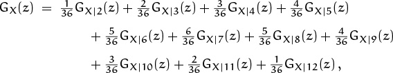
In the case of hashing, (8.92) tells us how to write down the pgf for probes in a successful search, if we let X = P and Y = K. For any fixed k between 1 and n, the random variable P|k is defined as a sum of independent random variables X₁ + · · · + X_k; this is (8.89). So it has the pgf

G_P|k(z)  =  

Therefore the pgf for P itself is clearly

where

is the pgf for the search probabilities s_k (divided by z for convenience).

“By clearly, I mean a good freshman should be able to do it, although it’s not completely trivial.”
    —Paul Erd˝os [94].

Good. We have a probability generating function for P; we can now find the mean and variance by differentiation. It’s somewhat easier to remove the z factor first, as we’ve done before, thus finding the mean and variance of P – 1 instead:

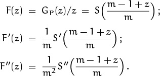
Therefore

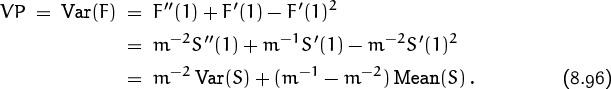
These are general formulas expressing the mean and variance of the number of probes P in terms of the mean and variance of the assumed search distribution S.

For example, suppose we have s_k = 1/n for 1 ≤ k ≤ n. This means we are doing a purely “random” successful search, with all keys in the table equally likely. Then S(z) is the uniform probability distribution U_n(z) in (8.32), and we have Mean(S) = (n – 1)/2, Var(S) = (n² – 1)/12. Hence

Once again we have gained the desired speedup factor of 1/m. If m ≈ n/ln n and n → ∞, the average number of probes per successful search in this case is about ln n, and the standard deviation is asymptotically (ln n)/.

On the other hand, we might suppose that s_k = (kH_n)^–1 for 1 ≤ k ≤ n; this distribution is called “Zipf’s law.” Then Mean (S) = n/H_n – 1, Var(S) = n(n + 1)/H_n – n²/. The average number of probes for m ≈ n/ln n as n → ∞ is approximately 2, with standard deviation asymptotic to .

In both cases the analysis allows the cautious souls among us, who fear the worst case, to rest easily: Chebyshev’s inequality tells us that the lists will be nice and short, except in extremely rare cases.

Case 2, continued: Variants of the variance.

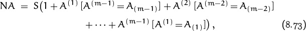
We have just computed the variance of the number of probes in a successful search, by considering P to be a random variable over a probability space with mⁿ·n elements (h₁, . . . , h_n; k). But we could have adopted another point of view: Each pattern (h₁, ..., h_n) of hash values defines a random variable P|(h₁, ..., h_n), representing the probes we make in a successful search of a particular hash table on n given keys. The average value of P|(h₁, ..., h_n),

can be said to represent the running time of a successful search. This quantity A(h₁, . . . , h_n) is a random variable that depends only on (h₁, . . . , h_n), not on the final component k. We can write it in the form

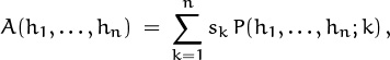
where P(h₁, . . . , h_n; k) is defined in (8.88), since P|(h₁, . . . , h_n) = p with probability

OK, gang, time to put on your skim suits again.
    — Friendly TA

The mean value of A(h₁, . . . , h_n), obtained by summing over all mⁿ possibilities (h₁, . . . , h_n) and dividing by mⁿ, will be the same as the mean value we obtained before in (8.95). But the variance of A(h₁, . . . , h_n) is something different; this is a variance of mⁿ averages, not a variance of mⁿ ·n probe counts. For example, if m = 1 (so that there is only one list), the “average” value A(h₁, . . . , h_n) = A(1, . . . , 1) is actually constant, so its variance VA is zero; but the number of probes in a successful search is not constant, so the variance VP is nonzero.

But the VP is nonzero only in an election year.

We can illustrate this difference between variances by carrying out the calculations for general m and n in the simplest case, when s_k = 1/n for 1 ≤ k ≤ n. In other words, we will assume temporarily that there is a uniform distribution of search keys. Any given sequence of hash values (h₁, . . . , h_n) defines m lists that contain respectively (n₁, n₂, . . . , n_m) entries for some numbers n_j, where

n₁ + n₂ + · · · + n_m = n.

A successful search in which each of the n keys in the table is equally likely will have an average running time of

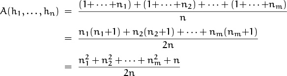
probes. Our goal is to calculate the variance of this quantity A(h₁, . . . , h_n), over the probability space consisting of all mⁿ sequences (h₁, . . . , h_n).

The calculations will be simpler, it turns out, if we compute the variance of a slightly different quantity,

We have

A(h₁, ..., h_n) = 1 + B(h₁, ..., h_n)/n,

hence the mean and variance of A satisfy

The probability that the list sizes will be n₁, n₂, . . . , n_m is the multinomial coefficient

divided by mⁿ; hence the pgf for B(h₁, . . . , h_n) is

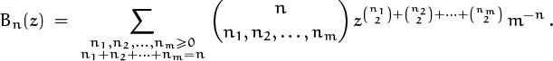
This sum looks a bit scary to inexperienced eyes, but our experiences in Chapter 7 have taught us to recognize it as an m-fold convolution. Indeed, if we consider the exponential super-generating function

we can readily verify that G(w, z) is simply an mth power:

As a check, we can try setting z = 1; we get G(w, 1) = (e^w)^m, so the coefficient of mⁿwⁿ/n! is B_n(1) = 1.

If we knew the values of and , we would be able to calculate Var(B_n). So we take partial derivatives of G(w, z) with respect to z:

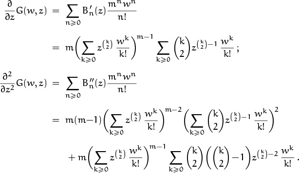
Complicated, yes; but everything simplifies greatly when we set z = 1. For example, we have

and it follows that

The expression for EA in (8.100) now gives EA = 1+(n–1)/2m, in agreement with (8.97).

The formula for involves the similar sum

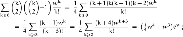
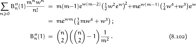
hence we find that

Now we can put all the pieces together and evaluate the desired variance VA. Massive cancellation occurs, and the result is surprisingly simple:

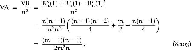
When such “coincidences” occur, we suspect that there’s a mathematical reason; there might be another way to attack the problem, explaining why the answer has such a simple form. And indeed, there is another approach (in exercise 61), which shows that the variance of the average successful search has the general form

when s_k is the probability that the kth-inserted element is being sought. Equation (8.103) is the special case s_k = 1/n for 1 ≤ k ≤ n.

Besides the variance of the average, we might also consider the average of the variance. In other words, each sequence (h₁, . . . , h_n) that defines a hash table also defines a probability distribution for successful searching, and the variance of this probability distribution tells how spread out the number of probes will be in different successful searches. For example, let’s go back to the case where we inserted n = 16 things into m = 10 lists:

(h₁, . . . , h₁₆) = 3 1 4 1 5 9 2 6 5 3 5 8 9 7 9 3;

(P₁, . . . , P₁₆) = 1 1 1 2 1 1 1 1 2 2 3 1 2 1 3 3.

Where have I seen that pattern before?

Where have I seen that graffito before?

IηνP_π.

A successful search in the resulting hash table has the pgf

G(3, 1, 4, 1, ..., 3)	=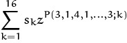
	=	s1z + s2z + s3z + s4z2 + · · · + s16z3.

We have just considered the average number of probes in a successful search of this table, namely A(3, 1, 4, 1, . . . , 3) = Mean (G(3, 1, 4, 1, . . . , 3)). We can also consider the variance,

This variance is a random variable, depending on (h₁, . . . , h_n), so it is natural to consider its average value.

In other words, there are three natural kinds of variance that we may wish to know, in order to understand the behavior of a successful search: The overall variance of the number of probes, taken over all (h₁, . . . , h_n) and k; the variance of the average number of probes, where the average is taken over all k and the variance is then taken over all (h₁, . . . , h_n); and the average of the variance of the number of the probes, where the variance is taken over all k and the average is then taken over all (h₁, . . . , h_n). In symbols, the overall variance is

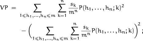
the variance of the average is

and the average of the variance is

It turns out that these three quantities are interrelated in a simple way:

In fact, conditional probability distributions always satisfy the identity

if X and Y are random variables in any probability space and if X takes real values. (This identity is proved in exercise 22.) Equation (8.105) is the special case where X is the number of probes in a successful search and Y is the sequence of hash values (h₁, . . . , h_n).

The general equation (8.106) needs to be understood carefully, because the notation tends to conceal the different random variables and probability spaces in which expectations and variances are being calculated. For each y in the range of Y, we have defined the random variable X|y in (8.91), and this random variable has an expected value E(X|y) depending on y. Now E(X|Y) denotes the random variable whose values are E(X|y) as y ranges over all possible values of Y, and V(E(X|Y)) is the variance of this random variable with respect to the probability distribution of Y. Similarly, E(V(X|Y)) is the average of the random variables V(X|y) as y varies. On the left of (8.106) is VX, the unconditional variance of X. Since variances are nonnegative, we always have

(Now is a good time to do warmup exercise 6.)

Case 1, again: Unsuccessful search revisited.

Let’s bring our microscopic examination of hashing to a close by doing one more calculation typical of algorithmic analysis. This time we’ll look more closely at the total running time associated with an unsuccessful search, assuming that the computer will insert the previously unknown key into its memory.

The insertion process in (8.83) has two cases, depending on whether j is negative or zero. We have j < 0 if and only if P = 0, since a negative value comes from the FIRST entry of an empty list. Thus, if the list was previously empty, we have P = 0 and we must set FIRST[h_n+1] := n + 1. (The new record will be inserted into position n + 1.) Otherwise we have P > 0 and we must set a NEXT entry to n + 1. These two cases may take different amounts of time; therefore the total running time for an unsuccessful search has the form

where α, β, and δ are constants that depend on the computer being used and on the way in which hashing is encoded in that machine’s internal language. It would be nice to know the mean and variance of T, since such information is more relevant in practice than the mean and variance of P.

P is still the number of probes.

So far we have used probability generating functions only in connection with random variables that take nonnegative integer values. But it turns out that we can deal in essentially the same way with

when X is any real-valued random variable, because the essential characteristics of X depend only on the behavior of G_X near z = 1, where powers of z are well defined. For example, the running time (8.108) of an unsuccessful search is a random variable, defined on the probability space of equally likely hash values (h₁, . . . , h_n, h_n+1) with 1 ≤ h_j ≤ m; we can consider the series

to be a pgf even when α, β, and δ are not integers. (In fact, the parameters α, β, δ are physical quantities that have dimensions of time; they aren’t even pure numbers! Yet we can use them in the exponent of z.) We can still calculate the mean and variance of T, by evaluating and and combining these values in the usual way.

The generating function for P instead of T is

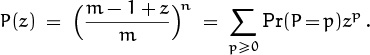
Therefore we have

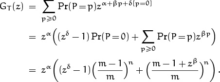
The determination of Mean(G_T ) and Var(G_T ) is now routine:

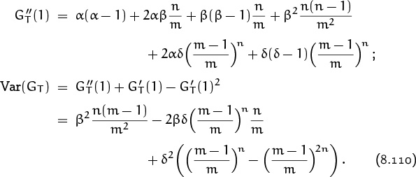
In Chapter 9 we will learn how to estimate quantities like this when m and n are large. If, for example, m = n and n → ∞, the techniques of Chapter 9 will show that the mean and variance of T are respectively α + β + δe^–1 + O(n^–1) and β² – 2βδe^–1 + δ²(e^–1 – e^–2) + O(n^–1). If m = n/ln n + O(1) and n → ∞ the corresponding results are

Mean(GT)	=	β ln n + α + O ([log n]2/n);
Var(GT)	=	β2 ln n + O ([log n]2/n).

Exercises

Warmups

1. What’s the probability of doubles in the probability distribution Pr₀₁ of (8.3), when one die is fair and the other is loaded? What’s the probability that S = 7 is rolled?

2. What’s the probability that the top and bottom cards of a randomly shuffled deck are both aces? (All 52! permutations have probability 1/52!.)

3. Stanford’s Concrete Math students were asked in 1979 to flip coins until they got heads twice in succession, and to report the number of flips required. The answers were

3, 2, 3, 5, 10, 2, 6, 6, 9, 2 .

Princeton’s Concrete Math students were asked in 1987 to do a similar thing, with the following results:

10, 2, 10, 7, 5, 2, 10, 6, 10, 2 .

Estimate the mean and variance, based on (a) the Stanford sample; (b) the Princeton sample.

Why only ten numbers?

The other students either weren’t empiricists or they were just too flipped out.

4. Let H(z) = F(z)/G(z), where F(1) = G(1) = 1. Prove that

Mean(H) = Mean(F) – Mean(G),

Var(H) = Var(F) – Var(G),

in analogy with (8.38) and (8.39), if the indicated derivatives exist at z = 1.

5. Suppose Alice and Bill play the game (8.78) with a biased coin that comes up heads with probability p. Is there a value of p for which the game becomes fair?

6. What does the conditional variance law (8.106) reduce to, when X and Y are independent random variables?

Basics

7. Show that if two dice are loaded with the same probability distribution, the probability of doubles is always at least .

8. Let A and B be events such that A ∪ B = Ω. Prove that

Pr(ω A ∩ B) = Pr(ω A) Pr(ω B) – Pr(ω ∉ A) Pr(ω ∉ B) .

9. Prove or disprove: If X and Y are independent random variables, then so are F(X) and G(Y), when F and G are any functions.

10. What’s the maximum number of elements that can be in the median set of a random variable X, according to definition (8.7)?

11. Construct a random variable that has finite mean and infinite variance.

12. a If P(z) is the pgf for the random variable X, prove that

Pr(X  ≤  r)  ≤  x^–rP(x)    for 0 < x ≤ 1;

Pr(X  ≥  r)  ≤  x^–rP(x)    for x ≥ 1.

(These important relations are called the tail inequalities.)

b In the special case P(z) = (1 + z)ⁿ/2ⁿ, use the first tail inequality to prove that ∑_k≤αn() ≤ 1/α^αn(1 – α)^(1–α)n when 0 < α < .

13. If X₁, . . . , X_2n are independent random variables with the same distribution, and if α is any real number whatsoever, prove that

14. Let F(z) and G(z) be probability generating functions, and let

H(z) = p F(z) + q G(z)

where p + q = 1. (This is called a mixture of F and G; it corresponds to flipping a coin and choosing probability distribution F or G depending on whether the coin comes up heads or tails.) Find the mean and variance of H in terms of p, q, and the mean and variance of F and G.

15. If F(z) and G(z) are probability generating functions, we can define another pgf H(z) by “composition”:

H(z) = F(G(z)).

Express Mean(H) and Var(H) in terms of Mean(F), Var(F), Mean(G), and Var(G). (Equation (8.93) is a special case.)

16. Find a closed form for the super generating function Σ_n≥0 F_n(z)wⁿ, when F_n(z) is the football-fixation generating function defined in (8.53).

17. Let X_n,p and Y_n,p have the binomial and negative binomial distributions, respectively, with parameters (n, p). (These distributions are defined in (8.57) and (8.60).) Prove that Pr(Y_n,p ≤ m) = Pr(X_m+n,p ≥ n). What identity in binomial coefficients does this imply?

18. A random variable X is said to have the Poisson distribution with mean μ if Pr(X = k) = e^–μμ^k/k! for all k ≥ 0.

a What is the pgf of such a random variable?

b What are its mean, variance, and other cumulants?

The distribution of fish per unit volume of water.

19. Continuing the previous exercise, let X₁ be a random Poisson variable with mean μ₁, and let X₂ be a random Poisson variable with mean μ₂, independent of X₁.

a What is the probability that X₁ + X₂ = n?

b What are the mean, variance, and other cumulants of 2X₁ + 3X₂?

20. Prove (8.74) and (8.75), the general formulas for mean and variance of the time needed to wait for a given pattern of heads and tails.

21. What does the value of N represent, if H and T are both set equal to in (8.77)?

22. Prove (8.106), the law of conditional expectations and variances.

Homework exercises

23. Let Pr₀₀ be the probability distribution of two fair dice, and let Pr₁₁ be the probability distribution of two loaded dice as given in (8.2). Find all events A such that Pr₀₀(A) = Pr₁₁(A). Which of these events depend only on the random variable S? (A probability space with Ω = D² has 2³⁶ events; only 2¹¹ of those events depend on S alone.)

24. Player J rolls 2n + 1 fair dice and removes those that come up . Player K then calls a number between 1 and 6, rolls the remaining dice, and removes those that show the number called. This process is repeated until no dice remain. The player who has removed the most total dice (n + 1 or more) is the winner.

a. What are the mean and variance of the total number of dice that J removes? Hint: The dice are independent.

b. What’s the probability that J wins, when n = 2?

25. Consider a gambling game in which you stake a given amount A and you roll a fair die. If k spots turn up, you multiply your stake by 2(k – 1)/5. (In particular, you double the stake whenever you roll , but you lose everything if you roll .) You can stop at any time and reclaim the current stake. What are the mean and variance of your stake after n rolls? (Ignore any effects of rounding to integer amounts of currency.)

26. Find the mean and variance of the number of l-cycles in a random permutation of n elements. (The football victory problem discussed in (8.23), (8.24), and (8.53) is the special case l = 1.)

27. Let X₁, X₂, . . . , X_n be independent samples of the random variable X. Equations (8.19) and (8.20) explain how to estimate the mean and variance of X on the basis of these observations; give an analogous formula for estimating the third cumulant κ₃. (Your formula should be an “unbiased” estimate, in the sense that its expected value should be κ₃.)

28. What is the average length of the coin-flipping game (8.78),

a given that Alice wins?

b given that Bill wins?

29. Alice, Bill, and Computer flip a fair coin until one of the respective patterns A = HHTH, B = HTHH, or C = THHH appears for the first time. (If only two of these patterns were involved, we know from (8.82) that A would probably beat B, that B would probably beat C, and that C would probably beat A; but all three patterns are simultaneously in the game.) What are each player’s chances of winning?

30. The text considers three kinds of variances associated with successful search in a hash table. Actually there are two more: We can consider the average (over k) of the variances (over h₁, . . . , h_n) of P(h₁, . . . , h_n; k); and we can consider the variance (over k) of the averages (over h₁, . . . , h_n). Evaluate these quantities.

31. An apple is located at vertex A of pentagon ABCDE, and a worm is located two vertices away, at C. Every day the worm crawls with equal probability to one of the two adjacent vertices. Thus after one day the worm is at vertex B or vertex D, each with probability . After two days, the worm might be back at C again, because it has no memory of previous positions. When it reaches vertex A, it stops to dine.

Schrödinger’s worm.

a What are the mean and variance of the number of days until dinner?

b Let p be the probability that the number of days is 100 or more. What does Chebyshev’s inequality say about p?

c What do the tail inequalities (exercise 12) tell us about p?

32. Alice and Bill are in the military, stationed in one of the five states Kansas, Nebraska, Missouri, Oklahoma, or Colorado. Initially Alice is in Nebraska and Bill is in Oklahoma. Every month each person is reassigned to an adjacent state, each adjacent state being equally likely. (Here’s a diagram of the adjacencies:

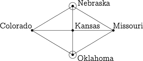
The initial states are circled.) For example, Alice is restationed after the first month to Colorado, Kansas, or Missouri, each with probability 1/3. Find the mean and variance of the number of months it takes Alice and Bill to find each other. (You may wish to enlist a computer’s help.)

Definitely a finite-state situation.

33. Are the random variables X₁ and X₂ in (8.89) independent?

34. Gina is a golfer who has probability p = .05 on each stroke of making a “supershot” that gains a stroke over par, probability q = .91 of making an ordinary shot, and probability r = .04 of making a “subshot” that costs her a stroke with respect to par. (Non-golfers: At each turn she advances 2, 1, or 0 steps toward her goal, with probability p, q, or r, respectively. On a par-m hole, her score is the minimum n such that she has advanced m or more steps after taking n turns. A low score is better than a high score.)

a. Show that Gina wins a par-4 hole more often than she loses, when she plays against a player who shoots par. (In other words, the probability that her score is less than 4 is greater than the probability that her score is greater than 4.)

b. Show that her average score on a par-4 hole is greater than 4. (Therefore she tends to lose against a “steady” player on total points, although she would tend to win in match play by holes.)

(Use a calculator for the numerical work on this problem.)

Exam problems

35. A die has been loaded with the probability distribution

Let S_n be the sum of the spots after this die has been rolled n times. Find a necessary and sufficient condition on the “loading distribution” such that the two random variables S_n mod 2 and S_n mod 3 are independent of each other, for all n.

36. The six faces of a certain die contain the spot patterns

instead of the usual through .

a. Show that there is a way to assign spots to the six faces of another die so that, when these two dice are thrown, the sum of spots has the same probability distribution as the sum of spots on two ordinary dice. (Assume that all 36 face pairs are equally likely.)

b. Generalizing, find all ways to assign spots to the 6n faces of n dice so that the distribution of spot sums will be the same as the distribution of spot sums on n ordinary dice. (Each face should receive a positive integer number of spots.)

37. Let p_n be the probability that exactly n tosses of a fair coin are needed before heads are seen twice in a row, and let q_n = Σ_k≥n pk. Find closed forms for both p_n and q_n in terms of Fibonacci numbers.

38. What is the probability generating function for the number of times you need to roll a fair die until all six faces have turned up? Generalize to m-sided fair dice: Give closed forms for the mean and variance of the number of rolls needed to see l of the m faces. What is the probability that this number will be exactly n?

39. A Dirichlet probability generating function has the form

Thus P(0) = 1. If X is a random variable with Pr(X = n) = p_n, express E(X), V(X), and E(ln X) in terms of P(z) and its derivatives.

40. The mth cumulant κ_m of the binomial distribution (8.57) has the form nf_m(p), where f_m is a polynomial of degree m. (For example, f₁(p) = p and f₂(p) = p – p², because the mean and variance are np and npq.)

a Find a closed form for the coefficient of p^k in f_m(p).

b Prove that f_m() = (2^m – 1)B_m/m + [m = 1], where B_m is the mth Bernoulli number.

41. Let the random variable X_n be the number of flips of a fair coin until heads have turned up a total of n times. Show that = (–1)ⁿ(ln 2 + H_n/2 – H_n).. Use the methods of Chapter 9 to estimate this value with an absolute error of O(n^–3).

42. A certain man has a problem finding work. If he is unemployed on any given morning, there’s constant probability p_h (independent of past history) that he will be hired before that evening; but if he’s got a job when the day begins, there’s constant probability p_f that he’ll be laid off by nightfall. Find the average number of evenings on which he will have a job lined up, assuming that he is initially employed and that this process goes on for n days. (For example, if n = 1 the answer is 1 – p_f.)

Does T_EX choose optimal line breaks?

43. Find a closed form for the pgf G_n(z) = Σ_k≥0pk,n^Zk, where p_k,n is the probability that a random permutation of n objects has exactly k cycles. What are the mean and standard deviation of the number of cycles?

44. The athletic department runs an intramural “knockout tournament” for 2ⁿ tennis players as follows. In the first round, the players are paired off randomly, with each pairing equally likely, and 2^n–1 matches are played. The winners advance to the second round, where the same process produces 2^n–2 winners. And so on; the kth round has 2^n–k randomly chosen matches between the 2^n–k+1 players who are still undefeated. The nth round produces the champion. Unbeknownst to the tournament organizers, there is actually an ordering among the players, so that x₁ is best, x₂ is second best, . . . , x₂n is worst. When x_j plays x_k and j < k, the winner is x_j with probability p and x_k with probability 1 – p, independent of the other matches. We assume that the same probability p applies to all j and k.

a. What’s the probability that x₁ wins the tournament?

b. What’s the probability that the nth round (the final match) is between the top two players, x₁ and x₂?

c. What’s the probability that the best 2^k players are the competitors in the kth-to-last round? (The previous questions were the cases k = 0 and k = 1.)

d. Let N(n) be the number of essentially different tournament results; two tournaments are essentially the same if the matches take place between the same players and have the same winners. Prove that N(n) = 2ⁿ!.

e. What’s the probability that x₂ wins the tournament?

f. Prove that if < p < 1, the probability that x_j wins is strictly greater than the probability that x_j+1 wins, for 1 ≤ j < 2ⁿ.

A peculiar set of tennis players.

45. True sherry is made in Spain according to a multistage system called “Solera.” For simplicity we’ll assume that the winemaker has only three barrels, called A, B, and C. Every year a third of the wine from barrel C is bottled and replaced by wine from B; then B is topped off with a third of the wine from A; finally A is topped off with new wine. Let A(z), B(z), C(z) be probability generating functions, where the coefficient of zⁿ is the fraction of n-year-old wine in the corresponding barrel just after the transfers have been made.

a. Assume that the operation has been going on since time immemorial, so that we have a steady state in which A(z), B(z), and C(z) are the same at the beginning of each year. Find closed forms for these generating functions.

b. Find the mean and standard deviation of the age of the wine in each barrel, under the same assumptions. What is the average age of the sherry when it is bottled? How much of it is exactly 25 years old?

c. Now take the finiteness of time into account: Suppose that all three barrels contained new wine at the beginning of year 0. What is the average age of the sherry that is bottled at the beginning of year n?

“Une rapide opération arithmétique montre que, grâce à cette ingénieuse cascade, les xérès ont toujours au moins trois ans. Pousser plus loin le calcul de leur âge donne le vertige.”
—Revue du vin de France (Nov 1984)

46. Stefan Banach used to carry two boxes of matches, each containing n matches initially. Whenever he needed a light he chose a box at random, each with probability , independent of his previous choices. After taking out a match he’d put the box back in its pocket (even if the box became empty—all famous mathematicians used to do this). When his chosen box was empty he’d throw it away and reach for the other box.

a. Once he found that the other box was empty too. What’s the probability that this occurs? (For n = 1 it happens half the time and for n = 2 it happens 3/8 of the time.) To answer this part, find a closed form for the generating function P(w, z) = Σ_m,n p_m,nw^mzⁿ, where p_m,n is the probability that, starting with m matches in one box and n in the other, both boxes are empty when an empty box is first chosen. Then find a closed form for p_n,n.

b. Generalizing your answer to part (a), find a closed form for the probability that exactly k matches are in the other box when an empty one is first thrown away.

c. Find a closed form for the average number of matches in that other box.

And for the number in the empty box.

47. Some physicians, collaborating with some physicists, recently discovered a pair of microbes that reproduce in a peculiar way. The male microbe, called a diphage, has two receptors on its surface; the female microbe, called a triphage, has three:

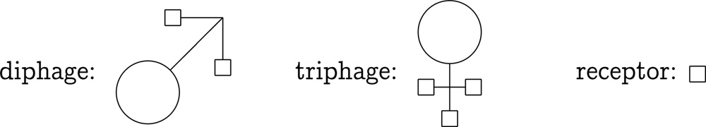
When a culture of diphages and triphages is irradiated with a psi-particle, exactly one of the receptors on one of the phages absorbs the particle; each receptor is equally likely. If it was a diphage receptor, that diphage changes to a triphage; if it was a triphage receptor, that triphage splits into two diphages. Thus if an experiment starts with one diphage, the first psi-particle changes it to a triphage, the second particle splits the triphage into two diphages, and the third particle changes one of the diphages to a triphage. The fourth particle hits either the diphage or the triphage; then there are either two triphages (probability ) or three diphages (probability ). Find a closed form for the average number of diphages present, if we begin with a single diphage and irradiate the culture n times with single psi-particles.

48. Five people stand at the vertices of a pentagon, throwing frisbees to each other.

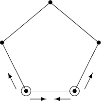
Or, if this pentagon is in Arlington, throwing missiles at each other.

They have two frisbees, initially at adjacent vertices as shown. In each time interval, each frisbee is thrown either to the left or to the right (along an edge of the pentagon) with equal probability. This process continues until one person is the target of two frisbees simultaneously; then the game stops. (All throws are independent of past history.)

a. Find the mean and variance of the number of pairs of throws.

b. Find a closed form for the probability that the game lasts more than 100 steps, in terms of Fibonacci numbers.

Frisbee is a trademark of Wham-O Manufacturing Company.

49. Luke Snowwalker spends winter vacations at his mountain cabin. The front porch has m pairs of boots and the back porch has n pairs. Every time he goes for a walk he flips a (fair) coin to decide whether to leave from the front porch or the back, and he puts on a pair of boots at that porch and heads off. There’s a 50/50 chance that he returns to each porch, independent of his starting point, and he leaves the boots at the porch he returns to. Thus after one walk there will be m + [–1, 0, or +1] pairs on the front porch and n – [–1, 0, or +1] pairs on the back porch. If all the boots pile up on one porch and if he decides to leave from the other, he goes without boots and gets frostbite, ending his vacation. Assuming that he continues his walks until the bitter end, let P_N(m, n) be the probability that he completes exactly N nonfrostbitten trips, starting with m pairs on the front porch and n on the back. Thus, if both m and n are positive,

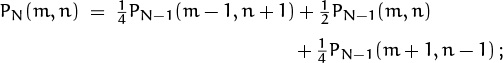
this follows because this first trip is either front/back, front/front, back/back, or back/front, each with probability , and N – 1 trips remain.

a. Complete the recurrence for P_N(m, n) by finding formulas that hold when m = 0 or n = 0. Use the recurrence to obtain equations that hold among the probability generating functions

b. Differentiate your equations and set z = 1, thereby obtaining relations among the quantities _,n(1). Solve these equations, thereby determining the mean number of trips before frostbite.

c. Show that g_m,n has a closed form if we substitute z = 1/cos² θ:

50. Consider the function

The purpose of this problem is to prove that H(z) = Σ_k≥0h_kZ^k is a probability generating function, and to obtain some basic facts about it.

a. Let (1 – z)^3/2(9 – z)^1/2 = Σ_k≥0 c_kz^k. Prove that c₀ = 3, c₁ = –14/3, c₂ = 37/27, and for all l ≥ 0. Hint: Use the identity

(9 – z)^1/2  =  3(1 – z)^1/2 (1 + z/(1 – z))^1/2

and expand the last factor in powers of z/(1 – z).

b. Use part (a) and exercise 5.81 to show that the coefficients of H(z) are all positive.

c. Prove the amazing identity

d. What are the mean and variance of H?

51. The state lottery in El Dorado uses the payoff distribution H defined in the previous problem. Each lottery ticket costs 1 doubloon, and the payoff is k doubloons with probability h_k. Your chance of winning with each ticket is completely independent of your chance with other tickets; in other words, winning or losing with one ticket does not affect your probability of winning with any other ticket you might have purchased in the same lottery.

a. Suppose you start with one doubloon and play this game. If you win k doubloons, you buy k tickets in the second game; then you take the total winnings in the second game and apply all of them to the third; and so on. If none of your tickets is a winner, you’re broke and you have to stop gambling. Prove that the pgf of your current holdings after n rounds of such play is

b. Let g_n be the probability that you lose all your money for the first time on the nth game, and let G(z) = g₁z + g₂z² + · · · . Prove that G(1) = 1. (This means that you’re bound to lose sooner or later, with probability 1, although you might have fun playing in the meantime.) What are the mean and the variance of G?

c. What is the average total number of tickets you buy, if you continue to play until going broke?

d. What is the average number of games until you lose everything if you start with two doubloons instead of just one?

A doubledoubloon.

Bonus problems

52. Show that the text’s definitions of median and mode for random variables correspond in some meaningful sense to the definitions of median and mode for sequences, when the probability space is finite.

53. Prove or disprove: If X, Y, and Z are random variables with the property that all three pairs (X, Y), (X, Z), and (Y, Z) are independent, then X + Y is independent of Z.

54. Equation (8.20) proves that the average value of X is VX. What is the variance X?

55. A normal deck of playing cards contains 52 cards, four each with face values in the set {A, 2, 3, 4, 5, 6, 7, 8, 9, 10, J, Q, K}. Let X and Y denote the respective face values of the top and bottom cards, and consider the following algorithm for shuffling:

S1 Permute the deck randomly so that each arrangement occurs with probability 1/52!.

S2 If X ≠ Y, flip a biased coin that comes up heads with probability p, and go back to step S1 if heads turns up. Otherwise stop.

Each coin flip and each permutation is assumed to be independent of all the other randomizations. What value of p will make X and Y independent random variables after this procedure stops?

56. Generalize the frisbee problem of exercise 48 from a pentagon to an m-gon. What are the mean and variance of the number of collision-free throws in general, when the frisbees are initially at adjacent vertices? Show that, if m is odd, the pgf for the number of throws can be written as a product of coin-flipping distributions:

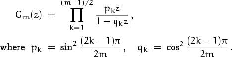
Hint: Try the substitution z = 1/cos² θ.

57. Prove that the Penney-ante pattern τ₁τ₂ . . . τ_l–1τ_l is always inferior to the pattern when a fair coin is flipped, if l ≥ 3.

58. Is there any sequence A = τ₁τ₂ . . . τ_l–1τ_l of l ≥ 3 heads and tails such that the sequences Hτ₁τ₂ . . . τ_l–1 and Tτ₁τ₂ . . . τ_l–1 both perform equally well against A in the game of Penney ante?

59. Are there patterns A and B of heads and tails such that A is longer than B, yet A appears before B more than half the time when a fair coin is being flipped?

60. Let k and n be fixed positive integers with k < n.

a. Find a closed form for the probability generating function

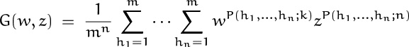
for the joint distribution of the numbers of probes needed to find the kth and nth items that have been inserted into a hash table with m lists.

b. Although the random variables P(h₁, . . . , h_n; k) and P(h₁, . . . , h_n; n) are dependent, show that they are somewhat independent:

E(P(h₁, . . . , h_n; k)P(h₁, . . . , h_n; n))
     =   (EP(h₁, . . . , h_n; k)) (EP(h₁, . . . , h_n; n))

61. Use the result of the previous exercise to prove (8.104).

62. Continuing exercise 47, find the variance of the number of diphages after n irradiations.

Research problem

63. The normal distribution is a non-discrete probability distribution characterized by having all its cumulants zero except the mean and the variance. Is there an easy way to tell if a given sequence of cumulants κ₁, κ₂, κ₃, . . . comes from a discrete distribution? (All the probabilities must be “atomic” in a discrete distribution.)