2. Sums
Sums are everywhere in mathematics, so we need basic tools to handle them. This chapter develops the notation and general techniques that make summation user-friendly.
2.1 Notation
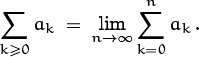
In Chapter 1 we encountered the sum of the first n integers, which we wrote out as 1 + 2 + 3 + · · · + (n – 1) + n. The ‘ · · · ’ in such formulas tells us to complete the pattern established by the surrounding terms. Of course we have to watch out for sums like 1 + 7 + · · · + 41.7, which are meaningless without a mitigating context. On the other hand, the inclusion of terms like 3 and (n – 1) was a bit of overkill; the pattern would presumably have been clear if we had written simply 1 + 2 + · · · + n. Sometimes we might even be so bold as to write just 1 + · · · + n.
We’ll be working with sums of the general form
where each ak is a number that has been defined somehow. This notation has the advantage that we can “see” the whole sum, almost as if it were written out in full, if we have a good enough imagination.
A term is how long this course lasts.
Each element ak of a sum is called a term. The terms are often specified implicitly as formulas that follow a readily perceived pattern, and in such cases we must sometimes write them in an expanded form so that the meaning is clear. For example, if
1 + 2 + · · · + 2n–1
is supposed to denote a sum of n terms, not of 2n–1, we should write it more explicitly as
20 + 21 + · · · + 2n–1.
The three-dots notation has many uses, but it can be ambiguous and a bit long-winded. Other alternatives are available, notably the delimited form

“Le signe ![]() indique que l’on doit donner au nombre entier i toutes ses valeurs 1, 2, 3, . . . , et prendre la somme des termes.”
indique que l’on doit donner au nombre entier i toutes ses valeurs 1, 2, 3, . . . , et prendre la somme des termes.”
—J. Fourier [127]
which is called Sigma-notation because it uses the Greek letter Σ (upper-case sigma). This notation tells us to include in the sum precisely those terms ak whose index k is an integer that lies between the lower and upper limits 1 and n, inclusive. In words, we “sum over k, from 1 to n.” Joseph Fourier introduced this delimited ∑-notation in 1820, and it soon took the mathematical world by storm.
Incidentally, the quantity after ∑ (here ak) is called the summand.
The index variable k is said to be bound to the ∑ sign in (2.2), because the k in ak is unrelated to appearances of k outside the Sigma-notation. Any other letter could be substituted for k here without changing the meaning of (2.2). The letter i is often used (perhaps because it stands for “index”), but we’ll generally sum on k since it’s wise to keep i for ![]() .
.
Well, I wouldn’t want to use a or n as the index variable instead of k in (2.2); those letters are “free variables” that do have meaning outside the ∑ here.
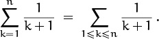
It turns out that a generalized Sigma-notation is even more useful than the delimited form: We simply write one or more conditions under the ∑, to specify the set of indices over which summation should take place. For example, the sums in (2.1) and (2.2) can also be written as
In this particular example there isn’t much difference between the new form and (2.2), but the general form allows us to take sums over index sets that aren’t restricted to consecutive integers. For example, we can express the sum of the squares of all odd positive integers below 100 as follows:
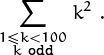
The delimited equivalent of this sum,
is more cumbersome and less clear. Similarly, the sum of reciprocals of all prime numbers between 1 and N is

the delimited form would require us to write

where pk denotes the kth prime and π(N) is the number of primes ≤ N. (Incidentally, this sum gives the approximate average number of distinct prime factors of a random integer near N, since about 1/p of those integers are divisible by p. Its value for large N is approximately ln ln N + M, where M ≈ 0.2614972128476427837554268386086958590515666 is Mertens’s constant [271]; ln x stands for the natural logarithm of x, and ln ln x stands for ln(ln x).)
The biggest advantage of general Sigma-notation is that we can manipulate it more easily than the delimited form. For example, suppose we want to change the index variable k to k + 1. With the general form, we have
The summation symbol looks like a distorted pacman.
it’s easy to see what’s going on, and we can do the substitution almost without thinking. But with the delimited form, we have
it’s harder to see what’s happened, and we’re more likely to make a mistake.
On the other hand, the delimited form isn’t completely useless. It’s nice and tidy, and we can write it quickly because (2.2) has seven symbols compared with (2.3)’s eight. Therefore we’ll often use ∑ with upper and lower delimiters when we state a problem or present a result, but we’ll prefer to work with relations-under-∑ when we’re manipulating a sum whose index variables need to be transformed.
A tidy sum.
The ∑ sign occurs more than 1000 times in this book, so we should be sure that we know exactly what it means. Formally, we write
That’s nothing. You should see how many times Σ appears in The Iliad.
as an abbreviation for the sum of all terms ak such that k is an integer satisfying a given property P(k). (A “property P(k)” is any statement about k that can be either true or false.) For the time being, we’ll assume that only finitely many integers k satisfying P(k) have ak ≠ 0; otherwise infinitely many nonzero numbers are being added together, and things can get a bit tricky. At the other extreme, if P(k) is false for all integers k, we have an “empty” sum; the value of an empty sum is defined to be zero.
A slightly modified form of (2.4) is used when a sum appears within the text of a paragraph rather than in a displayed equation: We write ‘∑P(k) ak’, attaching property P(k) as a subscript of ∑, so that the formula won’t stick out too much. Similarly, ‘![]() ’ is a convenient alternative to (2.2) when we want to confine the notation to a single line.
’ is a convenient alternative to (2.2) when we want to confine the notation to a single line.
People are often tempted to write
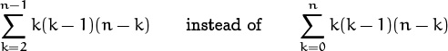
because the terms for k = 0, 1, and n in this sum are zero. Somehow it seems more efficient to add up n – 2 terms instead of n + 1 terms. But such temptations should be resisted; efficiency of computation is not the same as efficiency of understanding! We will find it advantageous to keep upper and lower bounds on an index of summation as simple as possible, because sums can be manipulated much more easily when the bounds are simple. Indeed, the form ![]() can even be dangerously ambiguous, because its meaning is not at all clear when n = 0 or n = 1 (see exercise 1). Zero-valued terms cause no harm, and they often save a lot of trouble.
can even be dangerously ambiguous, because its meaning is not at all clear when n = 0 or n = 1 (see exercise 1). Zero-valued terms cause no harm, and they often save a lot of trouble.
So far the notations we’ve been discussing are quite standard, but now we are about to make a radical departure from tradition. Kenneth E. Iverson introduced a wonderful idea in his programming language APL [191, page 11; see also 220], and we’ll see that it greatly simplifies many of the things we want to do in this book. The idea is simply to enclose a true-or-false statement in brackets, and to say that the result is 1 if the statement is true, 0 if the statement is false. For example,
Iverson’s convention allows us to express sums with no constraints whatever on the index of summation, because we can rewrite (2.4) in the form
Hey: The “Kronecker delta” that I’ve seen in other books (I mean δkn, which is 1 if k = n, 0 otherwise) is just a special case of Iverson’s convention: We can write [ k = n ] instead.
If P(k) is false, the term ak[P(k)] is zero, so we can safely include it among the terms being summed. This makes it easy to manipulate the index of summation, because we don’t have to fuss with boundary conditions.
“I am often surprised by new, important applications [of this notation].”
—B. de Finetti [123]
A slight technicality needs to be mentioned: Sometimes ak isn’t defined for all integers k. We get around this difficulty by assuming that [P(k)] is “very strongly zero” when P(k) is false; it’s so much zero, it makes ak[P(k)] equal to zero even when ak is undefined. For example, if we use Iverson’s convention to write the sum of reciprocal primes ≤ N as
there’s no problem of division by zero when p = 0, because our convention tells us that [0 prime][0 ≤ N]/0 = 0.
Let’s sum up what we’ve discussed so far about sums. There are two good ways to express a sum of terms: One way uses ‘ · · · ’, the other uses ‘∑’. The three-dots form often suggests useful manipulations, particularly the combination of adjacent terms, since we might be able to spot a simplifying pattern if we let the whole sum hang out before our eyes. But too much detail can also be overwhelming. Sigma-notation is compact, impressive to family and friends, and often suggestive of manipulations that are not obvious in three-dots form. When we work with Sigma-notation, zero terms are not generally harmful; in fact, zeros often make ∑-manipulation easier.
. . . and it’s less likely to lose points on an exam for “lack of rigor.”
2.2 Sums and Recurrences
OK, we understand now how to express sums with fancy notation. But how does a person actually go about finding the value of a sum? One way is to observe that there’s an intimate relation between sums and recurrences. The sum
is equivalent to the recurrence
(Think of Sn as not just a single number, but as a sequence defined for all n ≥ 0.)
Therefore we can evaluate sums in closed form by using the methods we learned in Chapter 1 to solve recurrences in closed form.
For example, if an is equal to a constant plus a multiple of n, the sum-recurrence (2.6) takes the following general form:
Proceeding as in Chapter 1, we find R1 = α + β + γ, R2 = α + 2β + 3γ, and so on; in general the solution can be written in the form
where A(n), B(n), and C(n) are the coefficients of dependence on the general parameters α, β, and γ.
The repertoire method tells us to try plugging in simple functions of n for Rn, hoping to find constant parameters α, β, and γ where the solution is especially simple. Setting Rn = 1 implies α = 1, β = 0, γ = 0; hence
A(n) = 1.
Setting Rn = n implies α = 0, β = 1, γ = 0; hence
B(n) = n.
Setting Rn = n2 implies α = 0, β = –1, γ = 2; hence
2C(n) – B(n) = n2
and we have C(n) = (n2 + n)/2. Easy as pie.
Actually easier; π = ![]() .
.
Therefore if we wish to evaluate
the sum-recurrence (2.6) boils down to (2.7) with α = β = a, γ = b, and the answer is aA(n) + aB(n) + bC(n) = a(n + 1) + b(n + 1)n/2.
Conversely, many recurrences can be reduced to sums; therefore the special methods for evaluating sums that we’ll be learning later in this chapter will help us solve recurrences that might otherwise be difficult. The Tower of Hanoi recurrence is a case in point:
T0 = 0;
Tn = 2Tn–1 + 1, for n > 0.
It can be put into the special form (2.6) if we divide both sides by 2n:
T0/20 = 0;
Tn/2n = Tn–1/2n –1 + 1/2n, for n > 0.
Now we can set Sn = Tn/2n, and we have
S0 = 0;
Sn = Sn–1 + 2–n, for n > 0.
It follows that
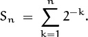
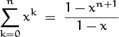
(Notice that we’ve left the term for k = 0 out of this sum.) The sum of the geometric series ![]() will be derived later in this chapter; it turns out to be
will be derived later in this chapter; it turns out to be ![]() . Hence Tn = 2nSn = 2n – 1.
. Hence Tn = 2nSn = 2n – 1.
We have converted Tn to Sn in this derivation by noticing that the recurrence could be divided by 2n. This trick is a special case of a general technique that can reduce virtually any recurrence of the form
to a sum. The idea is to multiply both sides by a summation factor, sn:
snanTn = snbnTn–1 + sncn.
This factor sn is cleverly chosen to make
snbn = sn–1an–1.
Then if we write Sn = snanTn we have a sum-recurrence,
Sn = Sn–1 + sncn.
Hence

and the solution to the original recurrence (2.9) is

For example, when n = 1 we get T1 = (s1b1T0+s1c1)/s1a1 = (b1T0+c1)/a1.
(The value of s1 cancels out, so it can be anything but zero.)
But how can we be clever enough to find the right sn? No problem: The relation sn = sn–1an–1/bn can be unfolded to tell us that the fraction
or any convenient constant multiple of this value, will be a suitable summation factor. For example, the Tower of Hanoi recurrence has an = 1 and bn = 2; the general method we’ve just derived says that sn = 2–n is a good thing to multiply by, if we want to reduce the recurrence to a sum. We don’t need a brilliant flash of inspiration to discover this multiplier.
We must be careful, as always, not to divide by zero. The summation-factor method works whenever all the a’s and all the b’s are nonzero.
Let’s apply these ideas to a recurrence that arises in the study of “quicksort,” one of the most important methods for sorting data inside a computer. The average number of comparison steps made by a typical implementation of quicksort when it is applied to n items in random order satisfies the recurrence
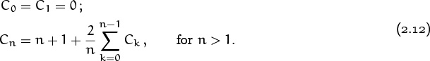
(Quicksort was invented by Hoare in 1962 [189].)
Hmmm. This looks much scarier than the recurrences we’ve seen before; it includes a sum over all previous values, and a division by n. Trying small cases gives us some data (C2 = 3, C3 = 6, ![]() ) but doesn’t do anything to quell our fears.
) but doesn’t do anything to quell our fears.
We can, however, reduce the complexity of (2.12) systematically, by first getting rid of the division and then getting rid of the ∑ sign. The idea is to multiply both sides by n, obtaining the relation
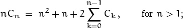
hence, if we replace n by n – 1,
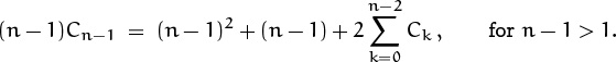
We can now subtract this equation from the first, and the ∑ sign disappears:
nCn – (n – 1)Cn–1 = 2n + 2Cn–1, for n > 2.
Therefore the original recurrence for Cn reduces to a much simpler one:
| C0 = | C1 = 0; C2 = 3; | |
| nCn = | (n + 1)Cn–1 + 2n, for n > 2. |
Progress. We’re now in a position to apply a summation factor, since this recurrence has the form of (2.9) with an = n, bn = n + 1, and
cn = 2n – 2[n = 1] + 2[n = 2].
The general method described on the preceding page tells us to multiply the recurrence through by some multiple of
The solution, according to (2.10), is therefore
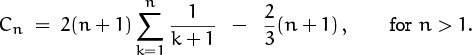
We started with a ∑ in the recurrence, and worked hard to get rid of it. But then after applying a summation factor, we came up with another ∑. Are sums good, or bad, or what?
The sum that remains is very similar to a quantity that arises frequently in applications. It arises so often, in fact, that we give it a special name and a special notation:

The letter H stands for “harmonic”; Hn is a harmonic number, so called because the kth harmonic produced by a violin string is the fundamental tone produced by a string that is 1/k times as long.
We can complete our study of the quicksort recurrence (2.12) by putting Cn into closed form; this will be possible if we can express Cn in terms of Hn. The sum in our formula for Cn is
We can relate this to Hn without much difficulty by changing k to k – 1 and revising the boundary conditions:
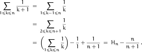
Alright! We have found the sum needed to complete the solution to (2.12): The average number of comparisons made by quicksort when it is applied to n randomly ordered items of data is
But your spelling is alwrong.
As usual, we check that small cases are correct: C2 = 3, C3 = 6.
2.3 Manipulation of Sums
The key to success with sums is an ability to change one ∑ into another that is simpler or closer to some goal. And it’s easy to do this by learning a few basic rules of transformation and by practicing their use.
Not to be confused with finance.
Let K be any finite set of integers. Sums over the elements of K can be transformed by using three simple rules:
My other math books have different definitions for these laws.
The distributive law allows us to move constants in and out of a ∑. The associative law allows us to break a ∑ into two parts, or to combine two ∑’s into one. The commutative law says that we can reorder the terms in any way we please; here p(k) is any permutation of the set of all integers. For example, if K = {–1, 0, +1} and if p(k) = –k, these three laws tell us respectively that
| ca–1 + ca0 + ca1 = c(a–1 + a0 + a1); | (distributive law) |
| (a–1 + b–1) + (a0 + b0) + (a1 + b1) | |
| = (a–1 + a0 + a1) + (b–1 + b0 + b1); | (associative law) |
| a–1 + a0 + a1 = a1 + a0 + a–1 . | (commutative law) |
Why not call it permutative instead of commutative?
Gauss’s trick in Chapter 1 can be viewed as an application of these three basic laws. Suppose we want to compute the general sum of an arithmetic progression,
By the commutative law we can replace k by n – k, obtaining
This is something like changing variables inside an integral, but easier.
These two equations can be added by using the associative law:
And we can now apply the distributive law and evaluate a trivial sum:
Dividing by 2, we have proved that

“What’s one and one and one and one and one and one and one and one and one and one?” “I don’t know,” said Alice. “I lost count.” “She can’t do Addition.”
—Lewis Carroll [50]
The right-hand side can be remembered as the average of the first and last terms, namely ![]() ), times the number of terms, namely (n + 1).
), times the number of terms, namely (n + 1).
It’s important to bear in mind that the function p(k) in the general commutative law (2.17) is supposed to be a permutation of all the integers. In other words, for every integer n there should be exactly one integer k such that p(k) = n. Otherwise the commutative law might fail; exercise 3 illustrates this with a vengeance. Transformations like p(k) = k + c or p(k) = c – k, where c is an integer constant, are always permutations, so they always work.
On the other hand, we can relax the permutation restriction a little bit: We need to require only that there be exactly one integer k with p(k) = n when n is an element of the index set K. If n ∉ K (that is, if n is not in K), it doesn’t matter how often p(k) = n occurs, because such k don’t take part in the sum. Thus, for example, we can argue that

since there’s exactly one k such that 2k = n when n ![]() K and n is even.
K and n is even.
Iverson’s convention, which allows us to obtain the values 0 or 1 from logical statements in the middle of a formula, can be used together with the distributive, associative, and commutative laws to deduce additional properties of sums. For example, here is an important rule for combining different sets of indices: If K and K′ are any sets of integers, then
Additional, eh?
This follows from the general formulas
and
Typically we use rule (2.20) either to combine two almost-disjoint index sets, as in
or to split off a single term from a sum, as in
(The two sides of (2.20) have been switched here.)
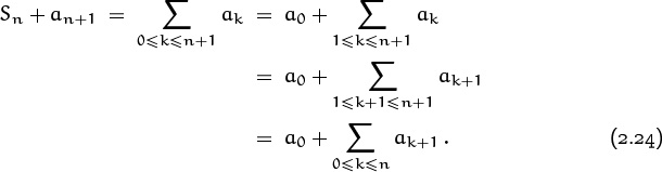
This operation of splitting off a term is the basis of a perturbation method that often allows us to evaluate a sum in closed form. The idea is to start with an unknown sum and call it Sn:
(Name and conquer.) Then we rewrite Sn+1 in two ways, by splitting off both its last term and its first term:
Now we can work on this last sum and try to express it in terms of Sn. If we succeed, we obtain an equation whose solution is the sum we seek.
For example, let’s use this approach to find the sum of a general geometric progression,
If it’s geometric, there should be a geometric proof.
The general perturbation scheme in (2.24) tells us that
and the sum on the right is x∑0≤k≤n axk = xSn by the distributive law. Therefore Sn + axn+1 = a + xSn, and we can solve for Sn to obtain

(When x = 1, the sum is of course simply (n + 1)a.) The right-hand side can be remembered as the first term included in the sum minus the first term excluded (the term after the last), divided by 1 minus the term ratio.
Ah yes, this formula was drilled into me in high school.
That was almost too easy. Let’s try the perturbation technique on a slightly more difficult sum,
In this case we have S0 = 0, S1 = 2, S2 = 10, S3 = 34, S4 = 98; what is the general formula? According to (2.24) we have
so we want to express the right-hand sum in terms of Sn. Well, we can break it into two sums with the help of the associative law,
and the first of the remaining sums is 2Sn. The other sum is a geometric progression, which equals (2 – 2n+2)/(1 – 2) = 2n+2 – 2 by (2.25). Therefore we have Sn + (n + 1)2n+1 = 2Sn + 2n+2 – 2, and algebra yields
Now we understand why S3 = 34: It’s 32 + 2, not 2·17.
A similar derivation with x in place of 2 would have given us the equation Sn + (n + 1)xn+1 = xSn + (x – xn+2)/(1 – x); hence we can deduce that

It’s interesting to note that we could have derived this closed form in a completely different way, by using elementary techniques of differential calculus. If we start with the equation
and take the derivative of both sides with respect to x, we get

because the derivative of a sum is the sum of the derivatives of its terms. We will see many more connections between calculus and discrete mathematics in later chapters.
2.4 Multiple Sums
The terms of a sum might be specified by two or more indices, not just by one. For example, here’s a double sum of nine terms, governed by two indices j and k:
Oh no, a nine-term governor.
Notice that this doesn’t mean to sum over all j ≥ 1 and all k ≤ 3.
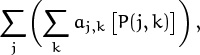
We use the same notations and methods for such sums as we do for sums with a single index. Thus, if P(j, k) is a property of j and k, the sum of all terms aj,k such that P(j, k) is true can be written in two ways, one of which uses Iverson’s convention and sums over all pairs of integers j and k:
Only one ∑ sign is needed, although there is more than one index of summation; ∑ denotes a sum over all combinations of indices that apply.
We also have occasion to use two ∑’s, when we’re talking about a sum of sums. For example,
is an abbreviation for
which is the sum, over all integers j, of ∑k aj,k [P(j, k)], the latter being the sum over all integers k of all terms aj,k for which P(j, k) is true. In such cases we say that the double sum is “summed first on k.” A sum that depends on more than one index can be summed first on any one of its indices.
Multiple ∑’s are evaluated right to left (inside-out).
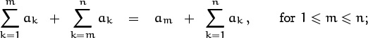
In this regard we have a basic law called interchanging the order of summation, which generalizes the associative law (2.16) we saw earlier:
The middle term of this law is a sum over two indices. On the left, ∑j ∑k stands for summing first on k, then on j. On the right, ∑k ∑j stands for summing first on j, then on k. In practice when we want to evaluate a double sum in closed form, it’s usually easier to sum it first on one index rather than on the other; we get to choose whichever is more convenient.
Who’s panicking? I think this rule is fairly obvious compared to some of the stuff in Chapter 1.
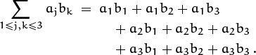
Sums of sums are no reason to panic, but they can appear confusing to a beginner, so let’s do some more examples. The nine-term sum we began with provides a good illustration of the manipulation of double sums, because that sum can actually be simplified, and the simplification process is typical of what we can do with ∑ ∑’s:
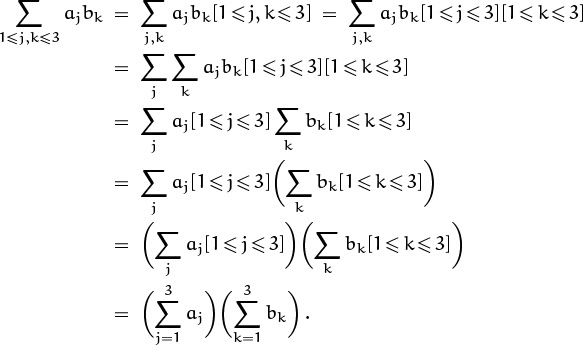
The first line here denotes a sum of nine terms in no particular order. The second line groups them in threes, (a1b1 + a1b2 + a1b3) + (a2b1 + a2b2 + a2b3) + (a3b1 + a3b2 + a3b3). The third line uses the distributive law to factor out the a’s, since aj and [1 ≤ j ≤ 3] do not depend on k; this gives a1(b1 + b2 + b3) + a2(b1 + b2 + b3) + a3(b1 + b2 + b3). The fourth line is the same as the third, but with a redundant pair of parentheses thrown in so that the fifth line won’t look so mysterious. The fifth line factors out the (b1 + b2 + b3) that occurs for each value of j: (a1 + a2 + a3)(b1 + b2 + b3). The last line is just another way to write the previous line. This method of derivation can be used to prove a general distributive law,
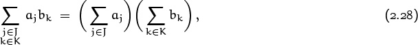
valid for all sets of indices J and K.
The basic law (2.27) for interchanging the order of summation has many variations, which arise when we want to restrict the ranges of the indices instead of summing over all integers j and k. These variations come in two flavors, vanilla and rocky road. First, the vanilla version:

This is just another way to write (2.27), since the Iversonian [j ![]() J, k
J, k ![]() K] factors into [j
K] factors into [j ![]() J][k
J][k ![]() K]. The vanilla-flavored law applies whenever the ranges of j and k are independent of each other.
K]. The vanilla-flavored law applies whenever the ranges of j and k are independent of each other.
The rocky-road formula for interchange is a little trickier. It applies when the range of an inner sum depends on the index variable of the outer sum:
Here the sets J, K(j), K′, and J′(k) must be related in such a way that
[j ![]() J][k
J][k ![]() K(j)] = [k
K(j)] = [k ![]() K′][j
K′][j ![]() J′(k)].
J′(k)].
A factorization like this is always possible in principle: We can let J = K′ be the set of all integers and K(j), J′(k) be sets corresponding to the property P(j, k) that governs a double sum. But there are important special cases where the sets J, K(j), K′, and J′(k) have a simple form. Such cases arise frequently in applications. For example, here’s a particularly useful factorization:
This Iversonian equation allows us to write

One of these two sums of sums is usually easier to evaluate than the other; we can use (2.32) to switch from the hard one to the easy one.
Let’s apply these ideas to a useful example. Consider the array

(Now is a good time to do warmup exercises 4 and 6.)
(Or to check out the Snickers bar languishing in the freezer.)
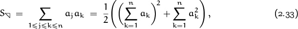
of n2 products ajak. Our goal will be to find a simple formula for
the sum of all elements on or above the main diagonal of this array. Because ajak = akaj, the array is symmetrical about its main diagonal; therefore ![]() will be approximately half the sum of all the elements (except for a fudge factor that takes account of the main diagonal).
will be approximately half the sum of all the elements (except for a fudge factor that takes account of the main diagonal).
Does rocky road have fudge in it?
Such considerations motivate the following manipulations. We have
because we can rename (j, k) as (k, j). Furthermore, since
[1 ≤ j ≤ k ≤ n] + [1 ≤ k ≤ j ≤ n] = [1 ≤ j, k ≤ n] + [1 ≤ j = k ≤ n] ,
we have
The first sum is ![]() , by the general distributive law (2.28). The second sum is
, by the general distributive law (2.28). The second sum is ![]() . Therefore we have
. Therefore we have
an expression for the upper triangular sum in terms of simpler single sums.
Encouraged by such success, let’s look at another double sum:
Again we have symmetry when j and k are interchanged:
So we can add S to itself, making use of the identity
[1 ≤ j < k ≤ n] + [1 ≤ k < j ≤ n] = [1 ≤ j, k ≤ n] – [1 ≤ j = k ≤ n]
to conclude that
The second sum here is zero; what about the first? It expands into four separate sums, each of which is vanilla flavored:
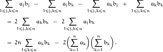
In the last step both sums have been simplified according to the general distributive law (2.28). If the manipulation of the first sum seems mysterious, here it is again in slow motion:
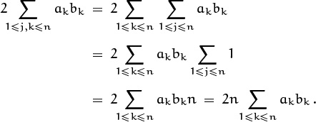
An index variable that doesn’t appear in the summand (here j) can simply be eliminated if we multiply what’s left by the size of that variable’s index set (here n).
Returning to where we left off, we can now divide everything by 2 and rearrange things to obtain an interesting formula:

This identity yields Chebyshev’s monotonic inequalities as a special case:
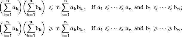
(Chebyshev [58] actually proved the analogous result for integrals instead of sums, ![]() , if f(x) and g(x) are monotone nondecreasing functions.)
, if f(x) and g(x) are monotone nondecreasing functions.)
(In general, if a1 ≤ · · · ≤ an and if p is a permutation of {1, . . . , n}, it’s not difficult to prove that the largest value of ![]() occurs when bp(1) ≤ · · · ≤ bp(n), and the smallest value occurs when bp(1) ≥ · · · ≥ bp(n).)
occurs when bp(1) ≤ · · · ≤ bp(n), and the smallest value occurs when bp(1) ≥ · · · ≥ bp(n).)
Multiple summation has an interesting connection with the general operation of changing the index of summation in single sums. We know by the commutative law that
if p(k) is any permutation of the integers. But what happens when we replace k by f(j), where f is an arbitrary function
f : J → K
that takes an integer j ![]() J into an integer f(j)
J into an integer f(j) ![]() K? The general formula for index replacement is
K? The general formula for index replacement is
where #f–(k) stands for the number of elements in the set
f–(k) = {j | f(j) = k},
that is, the number of values of j ![]() J such that f(j) equals k.
J such that f(j) equals k.
It’s easy to prove (2.35) by interchanging the order of summation,
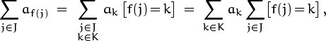
since ∑j![]() J[f(j) = k] = #f–(k). In the special case that f is a one-to-one correspondence between J and K, we have #f–(k) = 1 for all k, and the general formula (2.35) reduces to
J[f(j) = k] = #f–(k). In the special case that f is a one-to-one correspondence between J and K, we have #f–(k) = 1 for all k, and the general formula (2.35) reduces to
My other math teacher calls this a “bijection”; maybe I’ll learn to love that word some day.
And then again . . .
This is the commutative law (2.17) we had before, slightly disguised.
Our examples of multiple sums so far have all involved general terms like ak or bk. But this book is supposed to be concrete, so let’s take a look at a multiple sum that involves actual numbers:
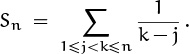
For example, S1 = 0; S2 = 1; ![]() .
.
Watch out—the authors seem to think that j, k, and n are “actual numbers.”
The normal way to evaluate a double sum is to sum first on j or first on k, so let’s explore both options.
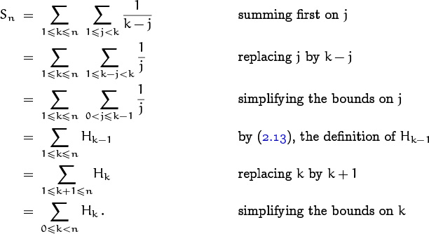
Alas! We don’t know how to get a sum of harmonic numbers into closed form.
Get out the whip.
If we try summing first the other way, we get
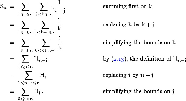
We’re back at the same impasse.
But there’s another way to proceed, if we replace k by k + j before deciding to reduce Sn to a sum of sums:
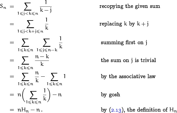
It’s smart to say k ≤ n instead of k ≤ n – 1 here. Simple bounds save energy.
Aha! We’ve found Sn. Combining this with the false starts we made gives us a further identity as a bonus:
We can understand the trick that worked here in two ways, one algebraic and one geometric. (1) Algebraically, if we have a double sum whose terms involve k+f(j), where f is an arbitrary function, this example indicates that it’s a good idea to try replacing k by k–f(j) and summing on j. (2) Geometrically, we can look at this particular sum Sn as follows, in the case n = 4:
| k = 1 k = 2 k = 3 k = 4 | |
| j = 1 | |
| j = 2 | |
| j = 3 | |
| j = 4 |
Our first attempts, summing first on j (by columns) or on k (by rows), gave us H1 + H2 + H3 = H3 + H2 + H1. The winning idea was essentially to sum by diagonals, getting ![]() .
.
2.5 General Methods
Now let’s consolidate what we’ve learned, by looking at a single example from several different angles. On the next few pages we’re going to try to find a closed form for the sum of the first n squares, which we’ll call ![]() :
:
We’ll see that there are at least eight different ways to solve this problem, and in the process we’ll learn useful strategies for attacking sums in general.
First, as usual, we look at some small cases.
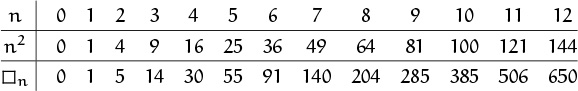
No closed form for ![]() is immediately evident; but when we do find one, we can use these values as a check.
is immediately evident; but when we do find one, we can use these values as a check.
Method 0: You could look it up.
A problem like the sum of the first n squares has probably been solved before, so we can most likely find the solution in a handy reference book. Sure enough, page 36 of the CRC Standard Mathematical Tables [28] has the answer:
Just to make sure we haven’t misread it, we check that this formula correctly gives ![]() . Incidentally, page 36 of the CRC Tables has further information about the sums of cubes, . . . , tenth powers.
. Incidentally, page 36 of the CRC Tables has further information about the sums of cubes, . . . , tenth powers.
The definitive reference for mathematical formulas is the Handbook of Mathematical Functions, edited by Abramowitz and Stegun [2]. Pages 813–814 of that book list the values of ![]() for n ≤ 100; and pages 804 and 809 exhibit formulas equivalent to (2.38), together with the analogous formulas for sums of cubes, . . . , fifteenth powers, with or without alternating signs.
for n ≤ 100; and pages 804 and 809 exhibit formulas equivalent to (2.38), together with the analogous formulas for sums of cubes, . . . , fifteenth powers, with or without alternating signs.
(Harder sums can be found in Hansen’s comprehensive table [178].)
But the best source for answers to questions about sequences is an amazing little book called the Handbook of Integer Sequences, by Sloane [330], which lists thousands of sequences by their numerical values. If you come up with a recurrence that you suspect has already been studied, all you have to do is compute enough terms to distinguish your recurrence from other famous ones; then chances are you’ll find a pointer to the relevant literature in Sloane’s Handbook. For example, 1, 5, 14, 30, . . . turns out to be Sloane’s sequence number 1574, and it’s called the sequence of “square pyramidal numbers” (because there are ![]() balls in a pyramid that has a square base of n2 balls). Sloane gives three references, one of which is to the handbook of Abramowitz and Stegun that we’ve already mentioned.
balls in a pyramid that has a square base of n2 balls). Sloane gives three references, one of which is to the handbook of Abramowitz and Stegun that we’ve already mentioned.
Still another way to probe the world’s store of accumulated mathematical wisdom is to use a computer program (such as Axiom, MACSYMA, Maple, or Mathematica) that provides tools for symbolic manipulation. Such programs are indispensable, especially for people who need to deal with large formulas.
It’s good to be familiar with standard sources of information, because they can be extremely helpful. But Method 0 isn’t really consistent with the spirit of this book, because we want to know how to figure out the answers by ourselves. The look-up method is limited to problems that other people have decided are worth considering; a new problem won’t be there.
Or, at least to problems having the same answers as problems that other people have decided to consider.
Method 1: Guess the answer, prove it by induction.
Perhaps a little bird has told us the answer to a problem, or we have arrived at a closed form by some other less-than-rigorous means. Then we merely have to prove that it is correct.
We might, for example, have noticed that the values of ![]() have rather small prime factors, so we may have come up with formula (2.38) as something that works for all small values of n. We might also have conjectured the equivalent formula
have rather small prime factors, so we may have come up with formula (2.38) as something that works for all small values of n. We might also have conjectured the equivalent formula
which is nicer because it’s easier to remember. The preponderance of the evidence supports (2.39), but we must prove our conjectures beyond all reasonable doubt. Mathematical induction was invented for this purpose.
“Well, Your Honor, we know that ![]() , so the basis is easy. For the inductive step, suppose that n > 0, and assume that (2.39) holds when n is replaced by n – 1. Since
, so the basis is easy. For the inductive step, suppose that n > 0, and assume that (2.39) holds when n is replaced by n – 1. Since
![]() n =
n = ![]() n–1 + n2,
n–1 + n2,
we have
| 3 |
= (n – 1)(n – |
| = (n3 – |
|
| = (n3 + |
|
| = n(n + |
Therefore (2.39) indeed holds, beyond a reasonable doubt, for all n ≥ 0.” Judge Wapner, in his infinite wisdom, agrees.
Induction has its place, and it is somewhat more defensible than trying to look up the answer. But it’s still not really what we’re seeking. All of the other sums we have evaluated so far in this chapter have been conquered without induction; we should likewise be able to determine a sum like ![]() from scratch. Flashes of inspiration should not be necessary. We should be able to do sums even on our less creative days.
from scratch. Flashes of inspiration should not be necessary. We should be able to do sums even on our less creative days.
Method 2: Perturb the sum.
So let’s go back to the perturbation method that worked so well for the geometric progression (2.25). We extract the first and last terms of ![]() +1 in order to get an equation for
+1 in order to get an equation for ![]() :
:
Oops—the ![]() ’s cancel each other. Occasionally, despite our best efforts, the perturbation method produces something like
’s cancel each other. Occasionally, despite our best efforts, the perturbation method produces something like ![]() , so we lose.
, so we lose.
Seems more like a draw.
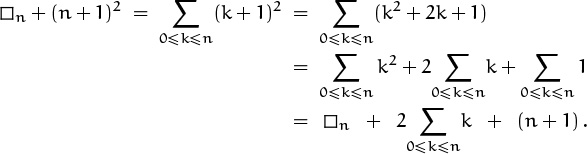
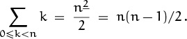
On the other hand, this derivation is not a total loss; it does reveal a way to sum the first few nonnegative integers in closed form,
even though we’d hoped to discover the sum of first integers squared. Could it be that if we start with the sum of the integers cubed, which we might call ![]() , we will get an expression for the integers squared? Let’s try it.
, we will get an expression for the integers squared? Let’s try it.
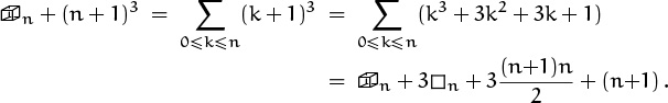
Sure enough, the ![]() ’s cancel, and we have enough information to determine
’s cancel, and we have enough information to determine ![]() without relying on induction:
without relying on induction:
| 3 |
= (n + 1)3 – 3(n + 1)n/2 – (n + 1) |
| = (n + 1)(n2 + 2n + 1 – |
Method 2′: Perturb your TA.
Method 3: Build a repertoire.
A slight generalization of the recurrence (2.7) will also suffice for summands involving n2. The solution to
will be of the general form
and we have already determined A(n), B(n), and C(n), because (2.40) is the same as (2.7) when δ = 0. If we now plug in Rn = n3, we find that n3 is the solution when α = 0, β = 1, γ = –3, δ = 3. Hence
3D(n) – 3C(n) + B(n) = n3;
this determines D(n).
We’re interested in the sum ![]() , which equals
, which equals ![]() ; thus we get
; thus we get ![]() if we set α = β = γ = 0 and δ = 1 in (2.40) and (2.41). Consequently
if we set α = β = γ = 0 and δ = 1 in (2.40) and (2.41). Consequently ![]() . We needn’t do the algebra to compute D(n) from B(n) and C(n), since we already know what the answer will be; but doubters among us should be reassured to find that
. We needn’t do the algebra to compute D(n) from B(n) and C(n), since we already know what the answer will be; but doubters among us should be reassured to find that
3D(n) = n3 + 3C(n) – B(n) = n3 + 3 ![]() – n = n(n+
– n = n(n+ ![]() )(n+1) .
)(n+1) .
Method 4: Replace sums by integrals.
People who have been raised on calculus instead of discrete mathematics tend to be more familiar with ∫ than with ∑, so they find it natural to try changing ∑ to ∫. One of our goals in this book is to become so comfortable with ∑ that we’ll think ∫ is more difficult than ∑ (at least for exact results). But still, it’s a good idea to explore the relation between ∑ and ∫, since summation and integration are based on very similar ideas.
In calculus, an integral can be regarded as the area under a curve, and we can approximate this area by adding up the areas of long, skinny rectangles that touch the curve. We can also go the other way if a collection of long, skinny rectangles is given: Since ![]() is the sum of the areas of rectangles whose sizes are 1 × 1, 1 × 4, . . . , 1 × n2, it is approximately equal to the area under the curve f(x) = x2 between 0 and n.
is the sum of the areas of rectangles whose sizes are 1 × 1, 1 × 4, . . . , 1 × n2, it is approximately equal to the area under the curve f(x) = x2 between 0 and n.
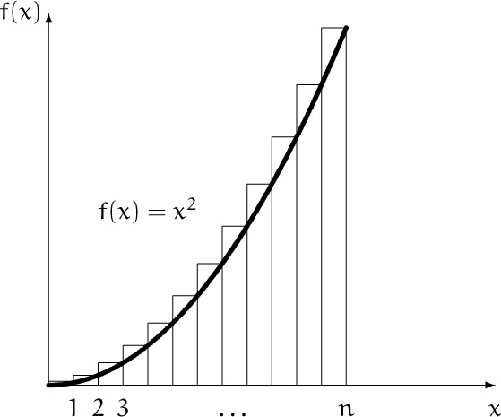
The horizontal scale here is ten times the vertical scale.
The area under this curve is ![]() ; therefore we know that
; therefore we know that ![]() is approximately
is approximately ![]() .
.
One way to use this fact is to examine the error in the approximation, ![]() . Since
. Since ![]() satisfies the recurrence
satisfies the recurrence ![]() , we find that En satisfies the simpler recurrence
, we find that En satisfies the simpler recurrence
| En = |
= En–1 + |
| = En–1 + n – |
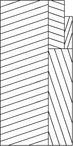
Another way to pursue the integral approach is to find a formula for En by summing the areas of the wedge-shaped error terms. We have
This is for people addicted to calculus.
Either way, we could find En and then ![]() .
.
Method 5: Expand and contract.
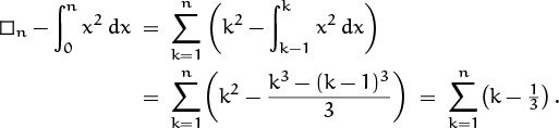
Yet another way to discover a closed form for ![]() is to replace the original sum by a seemingly more complicated double sum that can actually be simplified if we massage it properly:
is to replace the original sum by a seemingly more complicated double sum that can actually be simplified if we massage it properly:
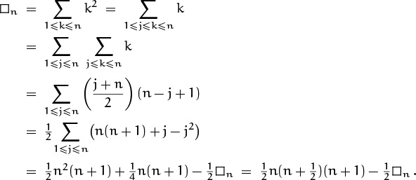
(The last step here is something like the last step of the perturbation method, because we get an equation with the unknown quantity on both sides.)
Going from a single sum to a double sum may appear at first to be a backward step, but it’s actually progress, because it produces sums that are easier to work with. We can’t expect to solve every problem by continually simplifying, simplifying, and simplifying: You can’t scale the highest mountain peaks by climbing only uphill.
Method 6: Use finite calculus.
Method 7: Use generating functions.
Stay tuned for still more exciting calculations of ![]() , as we learn further techniques in the next section and in later chapters.
, as we learn further techniques in the next section and in later chapters.
2.6 Finite and Infinite Calculus
We’ve learned a variety of ways to deal with sums directly. Now it’s time to acquire a broader perspective, by looking at the problem of summation from a higher level. Mathematicians have developed a “finite calculus,” analogous to the more traditional infinite calculus, by which it’s possible to approach summation in a nice, systematic fashion.
Infinite calculus is based on the properties of the derivative operator D, defined by
Finite calculus is based on the properties of the difference operator Δ, defined by
This is the finite analog of the derivative in which we restrict ourselves to positive integer values of h. Thus, h = 1 is the closest we can get to the “limit” as h → 0, and Δf(x) is the value of (f(x + h) – f(x))/h when h = 1.
The symbols D and Δ are called operators because they operate on functions to give new functions; they are functions of functions that produce functions. If f is a suitably smooth function of real numbers to real numbers, then Df is also a function from reals to reals. And if f is any real-to-real function, so is Δf. The values of the functions Df and Δf at a point x are given by the definitions above.
As opposed to a cassette function.
Early on in calculus we learn how D operates on the powers f(x) = xm. In such cases Df(x) = mxm–1. We can write this informally with f omitted,
D(xm) = mxm–1.
It would be nice if the Δ operator would produce an equally elegant result; unfortunately it doesn’t. We have, for example,
Δ(x3) = (x + 1)3 – x3 = 3x2 + 3x + 1.
Math power.
But there is a type of “mth power” that does transform nicely under Δ, and this is what makes finite calculus interesting. Such newfangled mth powers are defined by the rule
Notice the little straight line under the m; this implies that the m factors are supposed to go down and down, stepwise. There’s also a corresponding definition where the factors go up and up:
When m = 0, we have ![]() , because a product of no factors is conventionally taken to be 1 (just as a sum of no terms is conventionally 0).
, because a product of no factors is conventionally taken to be 1 (just as a sum of no terms is conventionally 0).
The quantity xm is called “x to the m falling,” if we have to read it aloud; similarly, ![]() is “x to the m rising.” These functions are also called falling factorial powers and rising factorial powers, since they are closely related to the factorial function n! = n(n – 1) . . . (1). In fact,
is “x to the m rising.” These functions are also called falling factorial powers and rising factorial powers, since they are closely related to the factorial function n! = n(n – 1) . . . (1). In fact, ![]() .
.
Several other notations for factorial powers appear in the mathematical literature, notably “Pochhammer’s symbol” (x)m for ![]() or xm; notations like x(m) or x(m) are also seen for xm. But the underline/overline convention is catching on, because it’s easy to write, easy to remember, and free of redundant parentheses.
or xm; notations like x(m) or x(m) are also seen for xm. But the underline/overline convention is catching on, because it’s easy to write, easy to remember, and free of redundant parentheses.
Falling powers xm are especially nice with respect to Δ. We have
| Δ(xm) | = (x + 1)m – xm |
| = (x + 1)x... (x – m + 2) – x... (x – m + 2)(x – m + 1) | |
| = mx(x – 1)...(x – m + 2), |
Mathematical terminology is sometimes crazy: Pochhammer [293] actually used the notation (x)m for the binomial coefficient (![]() ), not for factorial powers.
), not for factorial powers.
hence the finite calculus has a handy law to match D(xm) = mxm–1:
This is the basic factorial fact.
The operator D of infinite calculus has an inverse, the anti-derivative (or integration) operator ∫. The Fundamental Theorem of Calculus relates D to ∫:
g(x) = Df(x) if and only if ∫ g(x) dx = f(x) + C.
“Quemadmodum ad differentiam denotandam usi sumus signo Δ, ita summam indicabimus signo Σ. . . . ex quo æquatio z = Δy, si invertatur, dabit quoque y = Σz + C.”
—L. Euler [110]
Here ∫ g(x) dx, the indefinite integral of g(x), is the class of functions whose derivative is g(x). Analogously, Δ has as an inverse, the anti-difference (or summation) operator ∑; and there’s another Fundamental Theorem:
Here ∑g(x) δx, the indefinite sum of g(x), is the class of functions whose difference is g(x). (Notice that the lowercase δ relates to uppercase Δ as d relates to D.) The “C” for indefinite integrals is an arbitrary constant; the “C” for indefinite sums is any function p(x) such that p(x + 1) = p(x). For example, C might be the periodic function a + b sin 2πx; such functions get washed out when we take differences, just as constants get washed out when we take derivatives. At integer values of x, the function C is constant.
Now we’re almost ready for the punch line. Infinite calculus also has definite integrals: If g(x) = Df(x), then
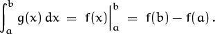
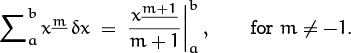
Therefore finite calculus—ever mimicking its more famous cousin—has definite sums: If g(x) = Δf(x), then
This formula gives a meaning to the notation ![]() , just as the previous formula defines
, just as the previous formula defines ![]() .
.
But what does ![]() really mean, intuitively? We’ve defined it by analogy, not by necessity. We want the analogy to hold, so that we can easily remember the rules of finite calculus; but the notation will be useless if we don’t understand its significance. Let’s try to deduce its meaning by looking first at some special cases, assuming that g(x) = Δf(x) = f(x + 1) – f(x). If b = a, we have
really mean, intuitively? We’ve defined it by analogy, not by necessity. We want the analogy to hold, so that we can easily remember the rules of finite calculus; but the notation will be useless if we don’t understand its significance. Let’s try to deduce its meaning by looking first at some special cases, assuming that g(x) = Δf(x) = f(x + 1) – f(x). If b = a, we have
Next, if b = a + 1, the result is
More generally, if b increases by 1, we have

These observations, and mathematical induction, allow us to deduce exactly what ![]() means in general, when a and b are integers with b ≥ a:
means in general, when a and b are integers with b ≥ a:

In other words, the definite sum is the same as an ordinary sum with limits, but excluding the value at the upper limit.
You call this a punch line?
Let’s try to recap this in a slightly different way. Suppose we’ve been given an unknown sum that’s supposed to be evaluated in closed form, and suppose we can write it in the form ![]() . The theory of finite calculus tells us that we can express the answer as f(b) – f(a), if we can only find an indefinite sum or anti-difference function f such that g(x) = f(x + 1) – f(x). One way to understand this principle is to write ∑a≤k<b g(k) out in full, using the three-dots notation:
. The theory of finite calculus tells us that we can express the answer as f(b) – f(a), if we can only find an indefinite sum or anti-difference function f such that g(x) = f(x + 1) – f(x). One way to understand this principle is to write ∑a≤k<b g(k) out in full, using the three-dots notation:

Everything on the right-hand side cancels, except f(b) – f(a); so f(b) – f(a) is the value of the sum. (Sums of the form ∑a≤k<b(f(k + 1) – f(k)) are often called telescoping, by analogy with a collapsed telescope, because the thickness of a collapsed telescope is determined solely by the outer radius of the outermost tube and the inner radius of the innermost tube.)
And all this time I thought it was telescoping because it collapsed from a very long expression to a very short one.
But rule (2.48) applies only when b ≥ a; what happens if b < a? Well, (2.47) says that we must have

This is analogous to the corresponding equation for definite integration. A similar argument proves ![]() , the summation analog of the identity
, the summation analog of the identity ![]() . In full garb,
. In full garb,
for all integers a, b, and c.
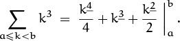
At this point a few of us are probably starting to wonder what all these parallels and analogies buy us. Well for one, definite summation gives us a simple way to compute sums of falling powers: The basic laws (2.45), (2.47), and (2.48) imply the general law
Others have been wondering this for some time now.

This formula is easy to remember because it’s so much like the familiar ![]() .
.
In particular, when m = 1 we have k1 = k, so the principles of finite calculus give us an easy way to remember the fact that
The definite-sum method also gives us an inkling that sums over the range 0 ≤ k < n often turn out to be simpler than sums over 1 ≤ k ≤ n; the former are just f(n) – f(0), while the latter must be evaluated as f(n + 1) – f(1).
Ordinary powers can also be summed in this new way, if we first express them in terms of falling powers. For example,
k2 = k2 + k1,
hence

Replacing n by n + 1 gives us yet another way to compute the value of our old friend ![]() in closed form.
in closed form.
With friends like this . . .
Gee, that was pretty easy. In fact, it was easier than any of the umpteen other ways that beat this formula to death in the previous section. So let’s try to go up a notch, from squares to cubes: A simple calculation shows that
k3 = k3 + 3k2 + k1.
(It’s always possible to convert between ordinary powers and factorial powers by using Stirling numbers, which we will study in Chapter 6.) Thus
Falling powers are therefore very nice for sums. But do they have any other redeeming features? Must we convert our old friendly ordinary powers to falling powers before summing, but then convert back before we can do anything else? Well, no, it’s often possible to work directly with factorial powers, because they have additional properties. For example, just as we have (x + y)2 = x2 + 2xy + y2, it turns out that (x + y)2 = x2 + 2x1y1 + y2, and the same analogy holds between (x + y)m and (x + y)m. (This “factorial binomial theorem” is proved in exercise 5.37.)
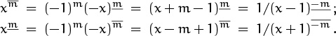
So far we’ve considered only falling powers that have nonnegative exponents. To extend the analogies with ordinary powers to negative exponents, we need an appropriate definition of xm for m < 0. Looking at the sequence
x3 = x(x – 1)(x – 2),
x2 = x(x – 1),
x1 = x,
x0 = 1,
we notice that to get from x3 to x2 to x1 to x0 we divide by x – 2, then by x – 1, then by x. It seems reasonable (if not imperative) that we should divide by x + 1 next, to get from x0 to x–1, thereby making x–1= 1/(x+1). Continuing, the first few negative-exponent falling powers are
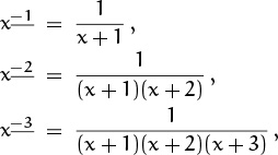
and our general definition for negative falling powers is
(It’s also possible to define falling powers for real or even complex m, but we will defer that until Chapter 5.)
How can a complex number be even?
With this definition, falling powers have additional nice properties. Perhaps the most important is a general law of exponents, analogous to the law
xm+n = xmxn
for ordinary powers. The falling-power version is
For example, x2+3 = x2(x – 2)3; and with a negative n we have
If we had chosen to define x–1 as 1/x instead of as 1/(x + 1), the law of exponents (2.52) would have failed in cases like m = –1 and n = 1. In fact, we could have used (2.52) to tell us exactly how falling powers ought to be defined in the case of negative exponents, by setting m = –n. When an existing notation is being extended to cover more cases, it’s always best to formulate definitions in such a way that general laws continue to hold.
Laws have their exponents and their detractors.
Now let’s make sure that the crucial difference property holds for our newly defined falling powers. Does Δxm = mxm–1 when m < 0? If m = –2, for example, the difference is
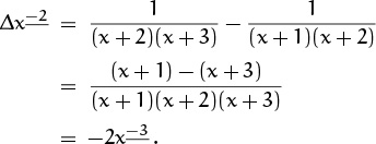
Yes—it works! A similar argument applies for all m < 0.
Therefore the summation property (2.50) holds for negative falling powers as well as positive ones, as long as no division by zero occurs:
But what about when m = –1? Recall that for integration we use
when m = –1. We’d like to have a finite analog of ln x; in other words, we seek a function f(x) such that
x–1 = ![]() = Δf(x) = f(x + 1) – f(x).
= Δf(x) = f(x + 1) – f(x).
It’s not too hard to see that
f(x) = ![]() +
+ ![]() + ··· +
+ ··· + ![]()
is such a function, when x is an integer, and this quantity is just the harmonic number Hx of (2.13). Thus Hx is the discrete analog of the continuous ln x. (We will define Hx for noninteger x in Chapter 6, but integer values are good enough for present purposes. We’ll also see in Chapter 9 that, for large x, the value of Hx – ln x is approximately 0.577 + 1/(2x). Hence Hx and ln x are not only analogous, their values usually differ by less than 1.)
0.577 exactly? Maybe they mean ![]() . Then again, maybe not.
. Then again, maybe not.
We can now give a complete description of the sums of falling powers:
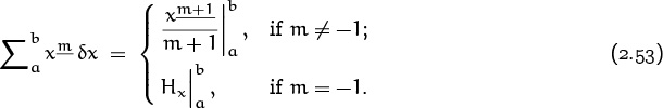
This formula indicates why harmonic numbers tend to pop up in the solutions to discrete problems like the analysis of quicksort, just as so-called natural logarithms arise naturally in the solutions to continuous problems.
Now that we’ve found an analog for ln x, let’s see if there’s one for ex. What function f(x) has the property that Δf(x) = f(x), corresponding to the identity Dex = ex? Easy:
f(x + 1) – f(x) = f(x) ![]() f(x + 1) = 2f(x);
f(x + 1) = 2f(x);
so we’re dealing with a simple recurrence, and we can take f(x) = 2x as the discrete exponential function.
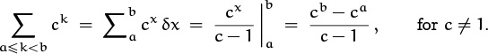
The difference of cx is also quite simple, for arbitrary c, namely
Δ(cx) = cx+1 – cx = (c – 1)cx.
Hence the anti-difference of cx is cx/(c – 1), if c ≠ 1. This fact, together with the fundamental laws (2.47) and (2.48), gives us a tidy way to understand the general formula for the sum of a geometric progression:
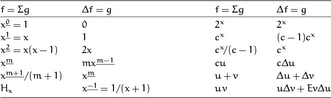
Every time we encounter a function f that might be useful as a closed form, we can compute its difference Δf = g; then we have a function g whose indefinite sum ∑g(x) δx is known. Table 55 is the beginning of a table of difference/anti-difference pairs useful for summation.
‘Table 55’ is on page 55. Get it?
Despite all the parallels between continuous and discrete math, some continuous notions have no discrete analog. For example, the chain rule of infinite calculus is a handy rule for the derivative of a function of a function; but there’s no corresponding chain rule of finite calculus, because there’s no nice form for Δf(g(x)). Discrete change-of-variables is hard, except in certain cases like the replacement of x by c ± x.
However, Δ(f(x) g(x)) does have a fairly nice form, and it provides us with a rule for summation by parts, the finite analog of what infinite calculus calls integration by parts. Let’s recall that the formula
D(uv) = u Dv + v Du
of infinite calculus leads to the rule for integration by parts,
∫ u Dv = uv – ∫ v Du ,
after integration and rearranging terms; we can do a similar thing in finite calculus.
We start by applying the difference operator to the product of two functions u(x) and v(x):

This formula can be put into a convenient form using the shift operator E, defined by
Ef(x) = f(x + 1).
Substituting Ev(x) for v(x+1) yields a compact rule for the difference of a product:
(The E is a bit of a nuisance, but it makes the equation correct.) Taking the indefinite sum on both sides of this equation, and rearranging its terms, yields the advertised rule for summation by parts:
Infinite calculus avoids E here by letting 1 → 0.
As with infinite calculus, limits can be placed on all three terms, making the indefinite sums definite.
I guess ex = 2x, for small values of 1.
This rule is useful when the sum on the left is harder to evaluate than the one on the right. Let’s look at an example. The function ∫ xex dx is typically integrated by parts; its discrete analog is ∑x2x δx, which we encountered earlier this chapter in the form ![]() . To sum this by parts, we let u(x) = x and Δv(x) = 2x; hence Δu(x) = 1, v(x) = 2x, and Ev(x) = 2x+1. Plugging into (2.56) gives
. To sum this by parts, we let u(x) = x and Δv(x) = 2x; hence Δu(x) = 1, v(x) = 2x, and Ev(x) = 2x+1. Plugging into (2.56) gives
∑x2x δx = x2x – ∑2x+1 δx = x2x – 2x+1 + C.
And we can use this to evaluate the sum we did before, by attaching limits:

It’s easier to find the sum this way than to use the perturbation method, because we don’t have to think.
The ultimate goal of mathematics is to eliminate all need for intelligent thought.
We stumbled across a formula for ∑0≤k<n Hk earlier in this chapter, and counted ourselves lucky. But we could have found our formula (2.36) systematically, if we had known about summation by parts. Let’s demonstrate this assertion by tackling a sum that looks even harder, ∑0≤k<n kHk. The solution is not difficult if we are guided by analogy with ∫ x ln x dx: We take u(x) = Hx and Δv(x) = x = x1, hence Δu(x) = x–1, v(x) = x2/2, Ev(x) = (x + 1)2/2, and we have
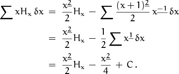
(In going from the first line to the second, we’ve combined two falling powers (x+1)2 x–1 by using the law of exponents (2.52) with m = –1 and n = 2.) Now we can attach limits and conclude that

2.7 Infinite Sums
When we defined ∑-notation at the beginning of this chapter, we finessed the question of infinite sums by saying, in essence, “Wait until later. For now, we can assume that all the sums we meet have only finitely many nonzero terms.” But the time of reckoning has finally arrived; we must face the fact that sums can be infinite. And the truth is that infinite sums are bearers of both good news and bad news.
This is finesse?
First, the bad news: It turns out that the methods we’ve used for manipulating ∑’s are not always valid when infinite sums are involved. But next, the good news: There is a large, easily understood class of infinite sums for which all the operations we’ve been performing are perfectly legitimate. The reasons underlying both these news items will be clear after we have looked more closely at the underlying meaning of summation.
Everybody knows what a finite sum is: We add up a bunch of terms, one by one, until they’ve all been added. But an infinite sum needs to be defined more carefully, lest we get into paradoxical situations.
For example, it seems natural to define things so that the infinite sum
S = 1 + ![]() +
+ ![]() +
+ ![]() +
+ ![]() +
+ ![]() + · · ·
+ · · ·
is equal to 2, because if we double it we get
2S = 2 + 1 + ![]() +
+ ![]() +
+ ![]() +
+ ![]() + · · · = 2 + S .
+ · · · = 2 + S .
On the other hand, this same reasoning suggests that we ought to define
T = 1 + 2 + 4 + 8 + 16 + 32 + · · ·
to be –1, for if we double it we get
2T = 2 + 4 + 8 + 16 + 32 + 64 + · · · = T – 1.
Something funny is going on; how can we get a negative number by summing positive quantities? It seems better to leave T undefined; or perhaps we should say that T = ∞, since the terms being added in T become larger than any fixed, finite number. (Notice that ∞ is another “solution” to the equation 2T = T – 1; it also “solves” the equation 2S = 2 + S.)
Sure: 1 + 2 + 4 + 8 + · · · is the “infinite precision” representation of the number –1, in a binary computer with infinite word size.
Let’s try to formulate a good definition for the value of a general sum ∑k![]() K ak, where K might be infinite. For starters, let’s assume that all the terms ak are nonnegative. Then a suitable definition is not hard to find: If there’s a bounding constant A such that
K ak, where K might be infinite. For starters, let’s assume that all the terms ak are nonnegative. Then a suitable definition is not hard to find: If there’s a bounding constant A such that
for all finite subsets F ⊂ K, then we define ∑k![]() K ak to be the least such A. (It follows from well-known properties of the real numbers that the set of all such A always contains a smallest element.) But if there’s no bounding constant A, we say that ∑k
K ak to be the least such A. (It follows from well-known properties of the real numbers that the set of all such A always contains a smallest element.) But if there’s no bounding constant A, we say that ∑k![]() K ak = ∞; this means that if A is any real number, there’s a set of finitely many terms ak whose sum exceeds A.
K ak = ∞; this means that if A is any real number, there’s a set of finitely many terms ak whose sum exceeds A.
The definition in the previous paragraph has been formulated carefully so that it doesn’t depend on any order that might exist in the index set K. Therefore the arguments we are about to make will apply to multiple sums with many indices k1, k2, . . . , not just to sums over the set of integers.
In the special case that K is the set of nonnegative integers, our definition for nonnegative terms ak implies that
The set K might even be uncountable. But only a countable number of terms can be nonzero, if a bounding constant A exists, because at most nA terms are ≥ 1/n.
Here’s why: Any nondecreasing sequence of real numbers has a limit (possibly ∞). If the limit is A, and if F is any finite set of nonnegative integers whose elements are all ≤ n, we have ![]() ; hence A = ∞ or A is a bounding constant. And if A′ is any number less than the stated limit A, then there’s an n such that
; hence A = ∞ or A is a bounding constant. And if A′ is any number less than the stated limit A, then there’s an n such that ![]() ; hence the finite set F = {0, 1, . . . , n} witnesses to the fact that A′ is not a bounding constant.
; hence the finite set F = {0, 1, . . . , n} witnesses to the fact that A′ is not a bounding constant.
We can now easily compute the value of certain infinite sums, according to the definition just given. For example, if ak = xk, we have
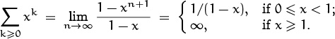
In particular, the infinite sums S and T considered a minute ago have the respective values 2 and ∞, just as we suspected. Another interesting example is
Now let’s consider the case that the sum might have negative terms as well as nonnegative ones. What, for example, should be the value of
If we group the terms in pairs, we get
(1 – 1) + (1 – 1) + (1 – 1) + · · · = 0 + 0 + 0 + · · · ,
so the sum comes out zero; but if we start the pairing one step later, we get
1 – (1 – 1) – (1 – 1) – (1 – 1) – · · · = 1 – 0 – 0 – 0 – · · ·;
the sum is 1.
“Aggregatum quantitatum a – a + a – a + a – a etc. nunc est = a, nunc = 0, adeoque continuata in infinitum serie ponendus = a/2, fateor acumen et veritatem animadversionis tuæ.”
—G. Grandi [163]
We might also try setting x = –1 in the formula ∑k≥0 xk = 1/(1 – x), since we’ve proved that this formula holds when 0 ≤ x < 1; but then we are forced to conclude that the infinite sum is ![]() , although it’s a sum of integers!
, although it’s a sum of integers!
Another interesting example is the doubly infinite ∑kak where ak = 1/(k + 1) for k ≥ 0 and ak = 1/(k – 1) for k < 0. We can write this as
If we evaluate this sum by starting at the “center” element and working outward,
we get the value 1; and we obtain the same value 1 if we shift all the parentheses one step to the left,
because the sum of all numbers inside the innermost n parentheses is
A similar argument shows that the value is 1 if these parentheses are shifted any fixed amount to the left or right; this encourages us to believe that the sum is indeed 1. On the other hand, if we group terms in the following way,
the nth pair of parentheses from inside out contains the numbers
We’ll prove in Chapter 9 that limn→∞(H2n – Hn+1) = ln 2; hence this grouping suggests that the doubly infinite sum should really be equal to 1 + ln 2.
There’s something flaky about a sum that gives different values when its terms are added up in different ways. Advanced texts on analysis have a variety of definitions by which meaningful values can be assigned to such pathological sums; but if we adopt those definitions, we cannot operate with ∑-notation as freely as we have been doing. We don’t need the delicate refinements of “conditional convergence” for the purposes of this book; therefore we’ll stick to a definition of infinite sums that preserves the validity of all the operations we’ve been doing in this chapter.
Is this the first page with no graffiti?
In fact, our definition of infinite sums is quite simple. Let K be any set, and let ak be a real-valued term defined for each k ![]() K. (Here ‘k’ might actually stand for several indices k1, k2, . . . , and K might therefore be multidimensional.) Any real number x can be written as the difference of its positive and negative parts,
K. (Here ‘k’ might actually stand for several indices k1, k2, . . . , and K might therefore be multidimensional.) Any real number x can be written as the difference of its positive and negative parts,
x = x+ – x–, where x+ = x·[x > 0] and x– = –x·[x < 0].
(Either x+ = 0 or x– = 0, or both.) We’ve already explained how to define values for the infinite sums ![]() and
and ![]() , because
, because ![]() and
and ![]() are nonnegative. Therefore our general definition is
are nonnegative. Therefore our general definition is
unless the right-hand sums are both equal to ∞. In the latter case, we leave ∑k![]() K ak undefined.
K ak undefined.
In other words, absolute convergence means that the sum of absolute values converges.
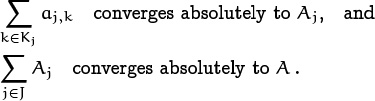
Let ![]() and
and ![]() . If A+ and A– are both finite, the sum ∑k
. If A+ and A– are both finite, the sum ∑k![]() K ak is said to converge absolutely to the value A = A+ – A–. If A+ = ∞ but A– is finite, the sum ∑k
K ak is said to converge absolutely to the value A = A+ – A–. If A+ = ∞ but A– is finite, the sum ∑k![]() K ak is said to diverge to + ∞. Similarly, if A– = ∞ but A+ is finite, ∑k
K ak is said to diverge to + ∞. Similarly, if A– = ∞ but A+ is finite, ∑k![]() K ak is said to diverge to –∞. If A+ = A– = ∞, all bets are off.
K ak is said to diverge to –∞. If A+ = A– = ∞, all bets are off.
We started with a definition that worked for nonnegative terms, then we extended it to real-valued terms. If the terms ak are complex numbers, we can extend the definition once again, in the obvious way: The sum ∑k![]() K ak is defined to be ∑k
K ak is defined to be ∑k![]() K ℜak + i ∑k
K ℜak + i ∑k![]() K ℑak, where ℜak and ℑak are the real and imaginary parts of ak—provided that both of those sums are defined. Otherwise ∑k
K ℑak, where ℜak and ℑak are the real and imaginary parts of ak—provided that both of those sums are defined. Otherwise ∑k![]() K ak is undefined. (See exercise 18.)
K ak is undefined. (See exercise 18.)
The bad news, as stated earlier, is that some infinite sums must be left undefined, because the manipulations we’ve been doing can produce inconsistencies in all such cases. (See exercise 34.) The good news is that all of the manipulations of this chapter are perfectly valid whenever we’re dealing with sums that converge absolutely, as just defined.
We can verify the good news by showing that each of our transformation rules preserves the value of all absolutely convergent sums. This means, more explicitly, that we must prove the distributive, associative, and commutative laws, plus the rule for summing first on one index variable; everything else we’ve done has been derived from those four basic operations on sums.
The distributive law (2.15) can be formulated more precisely as follows: If ∑k![]() K ak converges absolutely to A and if c is any complex number, then ∑k
K ak converges absolutely to A and if c is any complex number, then ∑k![]() K cak converges absolutely to cA. We can prove this by breaking the sum into real and imaginary, positive and negative parts as above, and by proving the special case in which c > 0 and each term ak is nonnegative. The proof in this special case works because ∑k
K cak converges absolutely to cA. We can prove this by breaking the sum into real and imaginary, positive and negative parts as above, and by proving the special case in which c > 0 and each term ak is nonnegative. The proof in this special case works because ∑k![]() F cak = c ∑k
F cak = c ∑k![]() F ak for all finite sets F; the latter fact follows by induction on the size of F.
F ak for all finite sets F; the latter fact follows by induction on the size of F.
The associative law (2.16) can be stated as follows: If ∑k![]() K ak and ∑k
K ak and ∑k![]() K bk converge absolutely to A and B, respectively, then ∑k
K bk converge absolutely to A and B, respectively, then ∑k![]() K (ak + bk) converges absolutely to A + B. This turns out to be a special case of a more general theorem that we will prove shortly.
K (ak + bk) converges absolutely to A + B. This turns out to be a special case of a more general theorem that we will prove shortly.
The commutative law (2.17) doesn’t really need to be proved, because we have shown in the discussion following (2.35) how to derive it as a special case of a general rule for interchanging the order of summation.
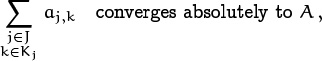
The main result we need to prove is the fundamental principle of multiple sums: Absolutely convergent sums over two or more indices can always be summed first with respect to any one of those indices. Formally, we shall prove that if J and the elements of {Kj | j ![]() J} are any sets of indices such that
J} are any sets of indices such that
Best to skim this page the first time you get here.
—Your friendly TA
then there exist complex numbers Aj for each j ![]() J such that
J such that
It suffices to prove this assertion when all terms are nonnegative, because we can prove the general case by breaking everything into real and imaginary, positive and negative parts as before. Let’s assume therefore that aj,k ≥ 0 for all pairs (j, k) ![]() M, where M is the master index set {(j, k) | j
M, where M is the master index set {(j, k) | j ![]() J, k
J, k ![]() Kj}.
Kj}.
We are given that ∑(j,k)![]() M aj,k is finite, namely that
M aj,k is finite, namely that
for all finite subsets F ⊆ M, and that A is the least such upper bound. If j is any element of J, each sum of the form ∑k![]() Fj aj,k where Fj is a finite subset of Kj is bounded above by A. Hence these finite sums have a least upper bound Aj ≥ 0, and ∑k
Fj aj,k where Fj is a finite subset of Kj is bounded above by A. Hence these finite sums have a least upper bound Aj ≥ 0, and ∑k![]() Kj aj,k = Aj by definition.
Kj aj,k = Aj by definition.
We still need to prove that A is the least upper bound of ∑j![]() G Aj, for all finite subsets G ⊆ J. Suppose that G is a finite subset of J with ∑j
G Aj, for all finite subsets G ⊆ J. Suppose that G is a finite subset of J with ∑j![]() G Aj = A′ > A. We can find finite subsets Fj ⊆ Kj such that ∑k
G Aj = A′ > A. We can find finite subsets Fj ⊆ Kj such that ∑k![]() Fj aj,k > (A/A′)Aj for each j
Fj aj,k > (A/A′)Aj for each j ![]() G with Aj > 0. There is at least one such j. But then ∑j
G with Aj > 0. There is at least one such j. But then ∑j![]() G,k
G,k![]() Fj aj,k > (A/A′) ∑j
Fj aj,k > (A/A′) ∑j![]() G Aj = A, contradicting the fact that we have ∑(j,k)
G Aj = A, contradicting the fact that we have ∑(j,k)![]() F aj,k ≤ A for all finite subsets F ⊆ M. Hence ∑j
F aj,k ≤ A for all finite subsets F ⊆ M. Hence ∑j![]() G Aj ≤ A, for all finite subsets G ⊆ J.
G Aj ≤ A, for all finite subsets G ⊆ J.
Finally, let A′ be any real number less than A. Our proof will be complete if we can find a finite set G ⊆ J such that ∑j![]() G Aj > A′. We know that there’s a finite set F ⊆ M such that ∑(j,k)
G Aj > A′. We know that there’s a finite set F ⊆ M such that ∑(j,k)![]() F aj,k > A′; let G be the set of j’s in this F, and let Fj = {k | (j, k)
F aj,k > A′; let G be the set of j’s in this F, and let Fj = {k | (j, k) ![]() F}. Then ∑j
F}. Then ∑j![]() G Aj ≥ ∑j
G Aj ≥ ∑j![]() G ∑k
G ∑k![]() Fj aj,k = ∑(j,k)
Fj aj,k = ∑(j,k)![]() F aj,k > A′; QED.
F aj,k > A′; QED.
OK, we’re now legitimate! Everything we’ve been doing with infinite sums is justified, as long as there’s a finite bound on all finite sums of the absolute values of the terms. Since the doubly infinite sum (2.58) gave us two different answers when we evaluated it in two different ways, its positive terms ![]() must diverge to ∞; otherwise we would have gotten the same answer no matter how we grouped the terms.
must diverge to ∞; otherwise we would have gotten the same answer no matter how we grouped the terms.
So why have I been hearing a lot lately about “harmonic convergence”?
Exercises
Warmups
1. What does the notation

mean?
2. Simplify the expression x · ([x > 0] – [x < 0]).
3. Demonstrate your understanding of ∑-notation by writing out the sums
in full. (Watch out—the second sum is a bit tricky.)
4. Express the triple sum
as a three-fold summation (with three ∑’s),
a. summing first on k, then j, then i;
b. summing first on i, then j, then k.
Also write your triple sums out in full without the ∑-notation, using parentheses to show what is being added together first.
5. What’s wrong with the following derivation?
6. What is the value of ∑k[1 ≤ j ≤ k ≤ n], as a function of j and n?
7. Let ∇f(x) = f(x) – f(x–1). What is ∇(x![]() )?
)?
Yield to the rising power.
8. What is the value of 0m, when m is a given integer?
9. What is the law of exponents for rising factorial powers, analogous to (2.52)? Use this to define ![]() .
.
10. The text derives the following formula for the difference of a product:
Δ(uv) = u Δv + Ev Δu.
How can this formula be correct, when the left-hand side is symmetric with respect to u and v but the right-hand side is not?
Basics
11. The general rule (2.56) for summation by parts is equivalent to
Prove this formula directly by using the distributive, associative, and commutative laws.
12. Show that the function p(k) = k + (–1)kc is a permutation of the set of all integers, whenever c is an integer.
13. Use the repertoire method to find a closed form for ![]() .
.
14. Evaluate ![]() by rewriting it as the multiple sum ∑1≤j≤k≤n 2k.
by rewriting it as the multiple sum ∑1≤j≤k≤n 2k.
15. Evaluate ![]() by the text’s Method 5 as follows: First write
by the text’s Method 5 as follows: First write ![]() ; then apply (2.33).
; then apply (2.33).
16. Prove that xm/(x – n)m = xn/(x – m)n, unless one of the denominators is zero.
17. Show that the following formulas can be used to convert between rising and falling factorial powers, for all integers m:
(The answer to exercise 9 defines ![]() .)
.)
18. Let ℜz and ℑz be the real and imaginary parts of the complex number z. The absolute value |z| is ![]() . A sum ∑k
. A sum ∑k![]() K ak of complex terms ak is said to converge absolutely when the real-valued sums ∑k
K ak of complex terms ak is said to converge absolutely when the real-valued sums ∑k![]() K ℜak and ∑k
K ℜak and ∑k![]() K ℑak both converge absolutely. Prove that ∑k
K ℑak both converge absolutely. Prove that ∑k![]() K ak converges absolutely if and only if there is a bounding constant B such that ∑k
K ak converges absolutely if and only if there is a bounding constant B such that ∑k![]() F |ak| ≤ B for all finite subsets F ⊆ K.
F |ak| ≤ B for all finite subsets F ⊆ K.
Homework exercises
19. Use a summation factor to solve the recurrence
| T0 = | 5; |
| 2Tn = | nTn–1 + 3 · n!, for n > 0. |
20. Try to evaluate ![]() by the perturbation method, but deduce the value of
by the perturbation method, but deduce the value of ![]() instead.
instead.
21. Evaluate the sums ![]() ,
, ![]() and
and ![]() by the perturbation method, assuming that n ≥ 0.
by the perturbation method, assuming that n ≥ 0.
22. Prove Lagrange’s identity (without using induction):
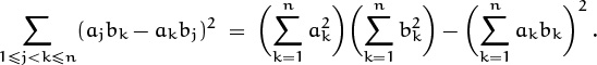
It’s hard to prove the identity of somebody who’s been dead for 175 years.
Prove, in fact, an identity for the more general double sum
23. Evaluate the sum ![]() in two ways:
in two ways:
a. Replace 1/k(k + 1) by the “partial fractions” 1/k – 1/(k + 1).
b. Sum by parts.
24. What is ∑0≤k<n Hk/(k + 1)(k + 2)? Hint: Generalize the derivation of (2.57).
25. The notation Πk![]() K ak means the product of the numbers ak for all k
K ak means the product of the numbers ak for all k ![]() K. Assume for simplicity that ak ≠ 1 for only finitely many k; hence infinite products need not be defined. What laws does this Π-notation satisfy, analogous to the distributive, associative, and commutative laws that hold for ∑?
K. Assume for simplicity that ak ≠ 1 for only finitely many k; hence infinite products need not be defined. What laws does this Π-notation satisfy, analogous to the distributive, associative, and commutative laws that hold for ∑?
This notation was introduced by Jacobi in 1829 [192].
26. Express the double product P = Π1≤j≤k≤n ajak in terms of the single product ![]() by manipulating Π-notation. (This exercise gives us a product analog of the upper-triangle identity (2.33).)
by manipulating Π-notation. (This exercise gives us a product analog of the upper-triangle identity (2.33).)
27. Compute Δ(cx), and use it to deduce the value of ![]() .
.
28. At what point does the following derivation go astray?
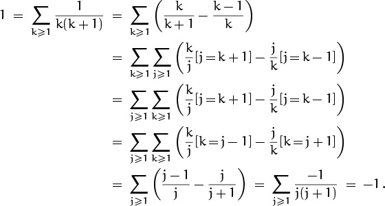
Exam problems
29. Evaluate the sum ![]() .
.
30. Cribbage players have long been aware that 15 = 7 + 8 = 4 + 5 + 6 = 1 + 2 + 3 + 4 + 5. Find the number of ways to represent 1050 as a sum of consecutive positive integers. (The trivial representation ‘1050’ by itself counts as one way; thus there are four, not three, ways to represent 15 as a sum of consecutive positive integers. Incidentally, a knowledge of cribbage rules is of no use in this problem.)
31. Riemann’s zeta function ζ(k) is defined to be the infinite sum
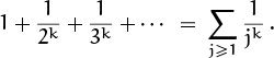
Prove that ∑k≥2 (ζ(k) – 1) = 1. What is the value of ∑k≥1 (ζ(2k) – 1)?
32. Let ![]() . Prove that
. Prove that
for all real x ≥ 0, and evaluate the sums in closed form.
Bonus problems
33. Let ∧k![]() K ak denote the minimum of the numbers ak (or their greatest lower bound, if K is infinite), assuming that each ak is either real or ±∞. What laws are valid for ∧-notation, analogous to those that work for ∑ and Π? (See exercise 25.)
K ak denote the minimum of the numbers ak (or their greatest lower bound, if K is infinite), assuming that each ak is either real or ±∞. What laws are valid for ∧-notation, analogous to those that work for ∑ and Π? (See exercise 25.)
The laws of the jungle.
34. Prove that if the sum ∑k![]() K ak is undefined according to (2.59), then it is extremely flaky in the following sense: If A– and A+ are any given real numbers, it’s possible to find a sequence of finite subsets F1 ⊂ F2 ⊂ F3 ⊂ · · · of K such that
K ak is undefined according to (2.59), then it is extremely flaky in the following sense: If A– and A+ are any given real numbers, it’s possible to find a sequence of finite subsets F1 ⊂ F2 ⊂ F3 ⊂ · · · of K such that
35. Prove Goldbach’s theorem

where P is the set of “perfect powers” defined recursively as follows:
P = { mn | m ≥ 2, n ≥ 2, m ∉ P }.
Perfect power corrupts perfectly.
36. Solomon Golomb’s “self-describing sequence” ![]() f(1), f(2), f(3), . . .
f(1), f(2), f(3), . . . ![]() is the only nondecreasing sequence of positive integers with the property that it contains exactly f(k) occurrences of k for each k. A few moments’ thought reveals that the sequence must begin as follows:
is the only nondecreasing sequence of positive integers with the property that it contains exactly f(k) occurrences of k for each k. A few moments’ thought reveals that the sequence must begin as follows:
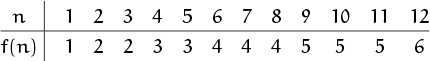
Let g(n) be the largest integer m such that f(m) = n. Show that
a. ![]()
b. ![]()
c. ![]()
Research problem
37. Will all the 1/k by 1/(k + 1) rectangles, for k ≥ 1, fit together inside a 1 by 1 square? (Recall that their areas sum to 1.)