
6.1 Introduction
A system is said to be stable if it does not exhibit large changes in its output for a small change in its input, initial conditions or its system parameters. In a stable system, the output is predictable and finite for a given input. The definition of stability depends on the type of system. Generally, the stability of a system is classified as stable, unstable and marginally stable.
A linear time-invariant system is said to be stable if the output remains bounded when the system is excited by a bounded input. This is called the Bounded-Input Bounded-Output (BIBO) stability criterion. Further,
- When there is no input, the system should produce a zero output irrespective of initial conditions. This is called the asymptotic stability criterion.
- If a bounded input is applied, the system remains stable for all values of system parameters. This is called the absolute stability.
- The stability of a system that exists for a particular range of parameters is called conditional stability.
- The relative stability indicates how close the system is to instability.
- Limitedly stable system produces output that has constant amplitude of oscillations.
The system can also be classified as Single-Input Single-Output (SISO), Multi-Input Multi-Output (MIMO), linear, nonlinear, time-invariant and time variant systems. In this chapter, the stability of linear SISO time-invariant systems has been discussed.
6.2 Concept of Stability
Let us consider the following two practical examples to have a clear idea on the stability of a system before going into the stability of linear SISO time-invariant systems.
Practical Example 1: Consider a ball that rests on different types of surfaces under the influence of the gravitational force as shown in Fig. 6.1.
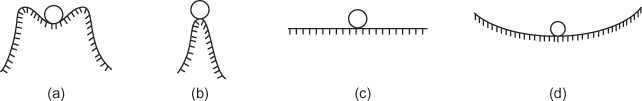
Fig. 6.1 ∣ Different equilibrium conditions: (a) Stable (asymptotic), (b) Unstable, (c) Marginally stable (non-asymptotic) and (d) Oscillatory
Stable System: A system is said to be stable if it maintains its equilibrium position (original position) when a small disturbance is applied to it. As shown in Fig. 6.1(a), even if the ball is disturbed, the equilibrium position will not change. Hence, the system is called asymptotically stable.
Unstable System: A system is said to be unstable if it attains a new equilibrium position that does not resemble the original equilibrium position when a small disturbance is applied to it. As shown in Fig. 6.1(b), even if the ball is slightly disturbed, it will upset the equilibrium condition and the ball will roll down from the hill and it will never return back to the equilibrium state. Hence, the system is called unstable.
Marginally Stable System: A system is said to be marginally stable if it attains a new equilibrium position that resembles the original equilibrium position when a small disturbance is applied to it. As shown in Fig. 6.1(c), when an impulsive force is applied, the ball will move for a fixed distance and then stop due to friction. Although the position is changed, the ball will come to a new equilibrium position. Hence, the system is called marginally or non-asymptotically stable.
Oscillatory System: As shown in Fig. 6.1(d), when we apply a disturbing force, the ball will move in both the directions (oscillatory motion). Eventually, these oscillations will cease due to the presence of friction and the ball will return back to its stable equilibrium state.
Practical Example 2: A conical structure shown in Fig. 6.2 is used to explain the concept of stability.

Fig. 6.2 ∣ Classification of system stability: Conical structure placed (a) on its base (stable), (b) on its tip (unstable) and (c) on its horizontal side (marginally stable)
Stable System: Consider a conical structure placed on its base as shown in Fig. 6.2(a). When a small disturbance is applied to the cone, a slight displacement can be observed before the cone returns back to its original position. Since the cone comes back its original position, it is said to be in the stable state.
Unstable System: Consider a conical structure placed on its tip as shown in Fig. 6.2(b). When a small disturbance is applied to the cone, it falls and rolls. Since the cone attains a new equilibrium point that does not resemble its original equilibrium point, it is said to be in the unstable state.
Marginally Stable System: Consider a conical structure placed on a horizontal surface as shown in Fig. 6.2(c). When a small disturbance is applied to the cone, a slight displacement can be observed before the cone attains a new position (equilibrium point). Since the new equilibrium point resembles the original equilibrium point, it is said to be in marginally stable state.
6.3 Stability of Linear Time-Invariant System
The most important specification of a system is its stability. Stability of the system depends on the total response of the system. The total response of the system is the summation of forced and natural responses of the system and is given by
![]()
The stability of the system can be defined based on either the natural response of the system or the total response of the system.
6.3.1 Stability Based on Natural Response of the System, c(t)natural
The stability of the linear time invariant (LTI) system based on the natural response of the system is shown in Table 6.1. It is clear that for a stable LTI system, only the forced response remains as it is when the natural response approaches zero as time tends to infinity.
Table 6.1 ∣ Classification of stability of LTI system

6.3.2 Stability Based on the Total Response of the System, c(t)
The above definition for the stability of the system is based on the natural response of the system. But when the total response of the system is given, it is very difficult to get the natural and forced responses separately. The stability of the system based on the total response is dependent on the input applied to the system and is shown in Table 6.2.
Table 6.2 ∣ Stability classification based on input and total response

The output or the total response of the system is said to be bounded, if the output or the total response of the system has a finite area under the curve. In addition, the output or the total response of the system is said to be unbounded, if the output or the total response of the system has an infinite area. The bounded and unbounded outputs are graphically shown in Table 6.2.
When the input to the system is unbounded, the output or the total response of the system is also unbounded. But from the total response of the system, it is very difficult to suggest whether the natural response of the system is unbounded or the forced response of the system is unbounded. Hence, for an unbounded input, we cannot suggest whether the system is stable, unstable or marginally stable.
Thus, the above examples define the stability of the system based on the bounded input and bounded output. Hence, this is known as BIBO stability.
6.4 Mathematical Condition for the Stability of the System
Let ![]()
![]() and
and ![]() be the input, output and the transfer function of the LTI SISO system respectively. The transfer function of the system is given by
be the input, output and the transfer function of the LTI SISO system respectively. The transfer function of the system is given by

For the impulse input, ![]() . Therefore,
. Therefore, ![]() . Taking inverse Laplace transform, we have
. Taking inverse Laplace transform, we have ![]() . For any input
. For any input ![]() , the output
, the output ![]() can be represented in the form of convolution as
can be represented in the form of convolution as
![]() (6.1)
(6.1)
where ![]() is the impulse response of the system output. If
is the impulse response of the system output. If ![]() and c(t) remain bounded, i.e., finite for all t, then
and c(t) remain bounded, i.e., finite for all t, then
![]()
The above equation may mathematically be derived as follows:
Taking absolute value on both sides of Eqn. (6.1), we obtain
![]()
According to an axiom, the absolute value of an integral cannot be greater than the integral of the absolute value of the integrand. Hence,
![]()
![]()
If ![]() is bounded, then
is bounded, then
![]() for
for ![]()
![]()
![]()
If ![]() remains bounded, then
remains bounded, then
![]() for
for ![]()
Combining the above two equations, we obtain
![]()
Hence,
![]()
6.5 Transfer Function of the System, G(s)
From Eqn. (6.1), it is clear that the mathematical condition for a stable system depends on the nature of ![]() . But the nature of
. But the nature of ![]() depends on the poles of the transfer function of the system G(s) or the roots of the characteristic equation of the system. The roots of the characteristic equation may be purely real, purely imaginary or complex conjugate with single root or multiple roots. In the section that follows, we will be discussing about the response of the system when an impulse signal is applied to the system.
depends on the poles of the transfer function of the system G(s) or the roots of the characteristic equation of the system. The roots of the characteristic equation may be purely real, purely imaginary or complex conjugate with single root or multiple roots. In the section that follows, we will be discussing about the response of the system when an impulse signal is applied to the system.
6.5.1 Effects of Location of Poles on Stability
Single Pole at the Origin: When there is a single pole at the origin, the transfer function is given by
For impulse response, ![]()
Then, ![]()
Therefore, ![]()
The location of the pole in the s-plane and its corresponding impulse response of the system having a single pole at the origin are shown in Fig. 6.3(a) and (b).

Fig. 6.3 ∣ (a) Location of pole in the s-plane and (b) Impulse response of the system having a single pole at the origin
A Pair of Poles at the Origin: When a pair of poles is located at the origin, the transfer function is
![]()
When ![]() , the corresponding impulse response is the ramp function, i.e.,
, the corresponding impulse response is the ramp function, i.e.,
The location of poles in the s-plane and its corresponding impulse response of the system having a pair of poles at the origin are shown in Fig. 6.4(a) and (b).
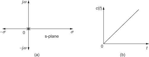
Fig. 6.4 ∣ (a) Location of poles in the s-plane and (b) Impulse response of the system having a pair of poles at the origin
Single Real Pole at the Right Half of the s-Plane: Let us consider the simple transfer function
![]()
When ![]() , the impulse response is
, the impulse response is ![]() .
.
The location of pole in the s-plane and its corresponding impulse response for the system having a single pole at the right half of the s-plane are shown in Fig. 6.5(a) and (b). The response clearly indicates that the output is not bounded and thus the system is unstable.

Fig. 6.5 ∣ (a) Location of a single pole in the right half of the s-plane and (b) Impulse response of the system having a single pole in the right half of the s-plane
Single Real Pole at the Left Half of the s-Plane: Let us consider the simple transfer function as

When ![]() , the impulse response is
, the impulse response is ![]() .
.
The location of pole in the s-plane and its corresponding impulse response for having a single pole at the left half of the s-plane are shown in Fig. 6.6(a) and (b). The response clearly indicates that the output decays to zero and the system is stable.

Fig. 6.6 ∣ (a) Location of a single pole in the left half of the s-plane and (b) Impulse response of the system having a single pole in the left half of the s-plane
A Pair of Poles on the Imaginary Axis: A transfer function of the system having a pair of poles on the imaginary axis is given by

When ![]() , the impulse response is
, the impulse response is ![]()
The location of poles in the s-plane and its corresponding impulse response are shown in Fig. 6.7(a) and (b). The response, which oscillates between +1 and −1, indicates that the system is marginally stable.

Fig. 6.7 ∣ (a) Location of poles in the s-plane and (b) Impulse response of the system having a pair of poles on the imaginary axis
Two Pairs of Repeated Poles on the Imaginary Axis: Let the transfer function be

When ![]() , the impulse response is
, the impulse response is ![]() .
.
The location of poles in the s-plane and its corresponding impulse response when there are two pairs of repeated poles on the imaginary axis are shown in Fig. 6.8(a) and (b). Here, the system is unstable if it possesses two pairs of repeated poles on the imaginary axis.

Fig. 6.8 ∣ (a) Location of poles in the s-plane and (b) Impulse response of the system when there are two pairs of repeated poles on the imaginary axis
A Pair of Complex Poles in the Right Half of the s-Plane: Let the transfer function be
When ![]() , the impulse response is
, the impulse response is ![]() .
.
The location of poles in the s-plane and its corresponding impulse response when there are repeated poles in the right half of the s-plane are shown in Fig. 6.9(a) and (b). The output clearly shows that the system having this kind of transfer function is unstable.

Fig. 6.9 ∣ (a) Location of poles in the s-plane and (b) Impulse response of the system when there are repeated poles in the right half of the s-plane
A Pair of Complex Poles in the Left Half of the s-Plane: Let the transfer function be

When ![]() , the impulse response is
, the impulse response is ![]() .
.
The location of poles in the s-plane and its corresponding impulse response when there are repeated poles in the left half of the s-plane are shown in Fig. 6.10(a) and (b). The output clearly shows that the system having this kind of transfer function is stable.

Fig. 6.10 ∣ (a) Location of poles in the s-plane and (b) Impulse response of the system when there are repeated poles in the left half of the s-plane
The mathematical expression for the response of a system and the graphical representation of the output response of the system corresponding to different types of roots are shown in Table 6.3.
Table 6.3 ∣ Nature of poles and the corresponding output responses of the system

Table 6.4 lists the conditions for stability of the system based on the location of poles in the s-plane.
Table 6.4 ∣ Location of poles in the s-plane and their stability
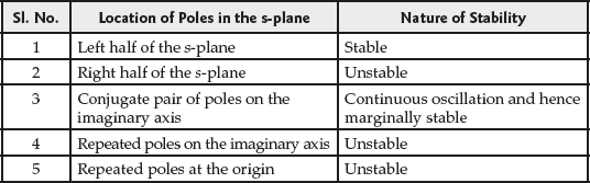
It is evident that the roots of the characteristic equation, i.e., the poles of the transfer function G(s) should lie in the left half of the s-plane for the system to be stable, or on the imaginary axis for the system to be marginally stable.
The conditions for stable and unstable regions in the s-plane are graphically shown in Fig. 6.11.

Fig. 6.11 ∣ Stable and unstable regions in the s-plane
6.6 Zero-Input Stability or Asymptotic Stability
Condition of asymptotic stability is defined by the following two responses of LTI system:
- Zero-State Response: Response of a system due to input alone with all the initial conditions of the system assigned to zero is known as zero-state response.
- Zero-Input Response: Response of a system due to initial conditions alone when the input of the system is assigned to zero is known as zero-input response. When the system is subjected to both input and initial conditions, the total response of the system can be obtained by using the principle of superposition as follows:
Total response = zero-state response + zero-input response.
Zero-Input Stability
Condition for stability of a system when the input is zero and when it is driven only by its initial conditions is known as zero-input stability or asymptotic stability. The zero-input stability also depends on the poles of the transfer function G(s). The output of the system due to initial condition when the input of nth order system is assumed to be zero is given by
![]() (6.2)
(6.2)
where 
and ![]() is the zero-input response due to
is the zero-input response due to ![]() .
.
A system is said to be zero-input stable if the zero-input response of the system ![]() , is subjected to finite initial conditions and
, is subjected to finite initial conditions and ![]() reaches zero as the time approaches infinity.
reaches zero as the time approaches infinity.
The condition for the system to be zero-input stable is given by
 , where M is a positive number.
-

From the second condition, it is clear that the zero-input stability is also known as asymptotic stability.
Taking absolute value on both sides of Eqn. (6.2), we obtain

As all the initial conditions are finite, the required condition for the system to be stable is given by
![]()
6.6.1 Importance of Asymptotic Stability
- The asymptotic stability depends on the poles of the transfer function of the system.
- The dependence of BIBO stability condition based on the location of poles of the system is applicable to asymptotic stability.
- If a system is BIBO stable, then it must be asymptotically stable.
Example 6.1: The transfer function of a closed-loop system is  Find the characteristic equation of the system.
Solution: The denominator of transfer function when equated to zero is called the characteristic equation of the system. Hence, the characteristic equation of the system is ![]()
Example 6.2: Comment on the stability of the systems whose transfer functions are given by
Solution:
- Poles are at
 . Hence, the system is asymptotically stable or simply stable.
 - Poles are at
 and
and  . Hence, the system is marginally stable.
 - Poles are at
 (double). Hence, the system is unstable.
 - Poles are at
 and
and  . Hence, the system is unstable.
 - Poles are at
 . Hence, the system is stable.
6.7 Relative Stability
Based on the location of poles of the transfer function, we can determine whether the system is stable, unstable or marginally stable. In practical systems, it is not sufficient to know that the system is stable, but a stable system must meet the requirements on relative stability which is a quantitative measure of how fast the transients die out in the system.
Relative stability is measured by relative settling times of each root or a pair of roots. A system is said to be relatively more stable if the settling time of the system is less when compared to other systems. The settling time of the system varies inversely to the real part of the roots. Hence, the roots located nearer to the imaginary axis will have a larger settling time and hence the system is relatively less stable.
For a system, the relative stability improves as the closed-loop poles of the transfer function moves away from the imaginary axis in the left half of the s-plane as shown in Fig. 6.12.

Fig. 6.12 ∣ Relation between the stability and closed-loop poles
Example 6.3: Consider the system, ![]() where
where ![]() is the real pole. Assume two real poles with values
is the real pole. Assume two real poles with values ![]() and
and ![]() where ∣p2∣ > ∣p1∣. Give your comments on their relative stability.
where ∣p2∣ > ∣p1∣. Give your comments on their relative stability.
Solution: Given two poles with values ![]() and
and ![]() where
where ![]() , the values of poles
, the values of poles ![]() and
and ![]() are plotted in the s-plane as shown in Fig. E6.3(a). For each value of the pole, when substituted in the system transfer function, the response of the system can be obtained as shown in Fig. E6.3(b). It is clear that the system with the pole value equal to
are plotted in the s-plane as shown in Fig. E6.3(a). For each value of the pole, when substituted in the system transfer function, the response of the system can be obtained as shown in Fig. E6.3(b). It is clear that the system with the pole value equal to ![]() settles much quicker than the system with the pole value equal to
settles much quicker than the system with the pole value equal to![]() . Hence, from the definition of relative stability, the system with lesser time is relatively more stable than the other one. From Fig. E6.3(a) and Fig. E6.3(b), it is inferred that the system with a less pole value is relatively more stable.
. Hence, from the definition of relative stability, the system with lesser time is relatively more stable than the other one. From Fig. E6.3(a) and Fig. E6.3(b), it is inferred that the system with a less pole value is relatively more stable.

Fig. E6.3 ∣ System with real poles: (a) location of poles in the s-plane and (b) their responses with corresponding settling times
Example 6.4: Consider the system ![]() where
where ![]() is the complex conjugate pole. Assume two conjugate poles with real parts having values
is the complex conjugate pole. Assume two conjugate poles with real parts having values ![]() and
and ![]() where
where ![]() . Give your comments on their relative stability.
. Give your comments on their relative stability.
Solution: Given two complex conjugate poles with real parts having values of ![]() and
and ![]() where
where ![]() , the poles are plotted in the s-plane as shown in Fig. E6.4(a). For each value of pole, when substituted in the system transfer function, the response of the system can be obtained as shown in Fig. E6.4(b). It is clear that the system with pole value equal to
, the poles are plotted in the s-plane as shown in Fig. E6.4(a). For each value of pole, when substituted in the system transfer function, the response of the system can be obtained as shown in Fig. E6.4(b). It is clear that the system with pole value equal to ![]() settles much quicker than the system with pole value equal to
settles much quicker than the system with pole value equal to ![]() Hence, from the definition of relative stability, the system with lesser time is relatively more stable than the other one. From Fig. E6.4(a) and (b), it is inferred that the system whose pole value has a lesser value or the complex conjugate pole which is at a higher distance from the imaginary axis is relatively more stable.
Hence, from the definition of relative stability, the system with lesser time is relatively more stable than the other one. From Fig. E6.4(a) and (b), it is inferred that the system whose pole value has a lesser value or the complex conjugate pole which is at a higher distance from the imaginary axis is relatively more stable.

Fig. E6.4 ∣ System with complex conjugate poles: (a) location of poles in the s-plane and (b) their responses with corresponding settling times.
Example 6.5: The transfer function of a plant is  Find the second-order approximation of
 ![]() using dominant pole concept.
using dominant pole concept.
Solution: Given 

In the given transfer function, denominator is ![]() . It can be observed that the pole at
. It can be observed that the pole at ![]() is more dominant than the pole at
is more dominant than the pole at ![]() . Thus the second-order approximation is obtained.
. Thus the second-order approximation is obtained.
6.8 Methods for Determining the Stability of the System
When the characteristic equation of the system has known parameters, it is very easy to determine the stability of the system by finding the roots of characteristic equation. But when there are some unknown parameters in the equation, the stability of the system can be determined by using the methods given below.
- Routh–Hurwitz Criterion: Routh–Hurwitz criterion was developed independently by E. J. Routh (1892) in the United States of America and A. Hurwitz (1895) in Germany, which is useful to determine the stability of the system without solving the characteristic equation. This is an algebraic method that provides stability information of the system that has the characteristic equation with constant coefficients. It indicates the number of roots of the characteristic equation, which lie on the imaginary axis and in the left half and right half of the s-plane without solving it.
- Root Locus Technique: The technique which was first introduced by W. R. Evans in 1946 for determining the trajectories of the roots of the characteristic equation is known as root locus technique. Root locus technique is also used for analyzing the stability of the system with variation of gain of the system.
- Bode Plot: This is a plot of magnitude of the transfer function in decibel versus ω and the phase angle versus
 , as
, as  is varied from zero to infinity. By observing the behaviour of the plots, the stability of the system is determined.
 - Polar Plot: It provides the magnitude and phase relationship between the input and output response of the system, i.e., a plot of magnitude versus phase angle in the polar co-ordinates. The magnitude and phase angle of the output response is obtained from the steady-state response of a system on a complex plane when it is subjected to sinusoidal input.
- Nyquist Criterion: This is a semi-graphical method that gives the difference between the number of poles and zeros of the closed-loop transfer function of the system, which are in the right half of the s-plane.
The Routh–Hurwitz criterion for examining the stability of the system is discussed in the following section.
6.9 Routh–Hurwitz Criterion
Routh–Hurwitz criterion gives the information on the absolute stability of a system without any necessity to solve for the closed-loop system poles. This method helps in determining the number of closed-loop system poles in the left half of the s-plane, the right half of the s-plane and on the ![]() axis, but not their co-ordinates. Stability of the system can be determined by the location of poles.
axis, but not their co-ordinates. Stability of the system can be determined by the location of poles.
The transfer function of the linear closed loop system is represented as

where an and bm are the real coefficients and n, m = 0, 1, 2,... .
Let ![]() be the characteristic equation of the given linear system. When this characteristic equation is solved for the roots, it gives the closed-loop poles of the given linear system, which decides the absolute stability of the system.
be the characteristic equation of the given linear system. When this characteristic equation is solved for the roots, it gives the closed-loop poles of the given linear system, which decides the absolute stability of the system.
In order that all the roots of the characteristic equation be pseudo-negative, two conditions are necessary although they are not sufficient. These conditions are as follows:
- All the coefficients from
 to
to  of the characteristic equation must have the same sign.
 - All the coefficients from
 to
to  of the characteristic equation must be present.
These conditions are based on the laws of algebra which relate the coefficients of the characteristic equation as follows:
![]()
![]()
![]() etc.
etc.
![]()
Thus, if the above ratios are positive and non-zero, then all the roots of the characteristic equation lie in the left half of the s-plane.
Example 6.6: For the characteristic equation F(s) = s4 + 4s3 + 3s + 6, check whether it has roots in the left half of the s-plane.
Solution: Given the characteristic equation ![]() . It does not have the term
. It does not have the term ![]() Hence, it does not have all the roots in the left half of the s-plane. Therefore, there are some pseudo-negative roots.
Hence, it does not have all the roots in the left half of the s-plane. Therefore, there are some pseudo-negative roots.
Example 6.7: For the characteristic equation F(s) = 2s4 − 5s3 + 2s2 + 7s + 3, check whether it has roots in the left half of the s-plane.
Solution: In the given characteristic equation ![]() , the coefficient of
, the coefficient of ![]() is negative, whereas all others are positive. Hence, it does not have all the roots in the left half of the s-plane.
is negative, whereas all others are positive. Hence, it does not have all the roots in the left half of the s-plane.
6.9.1 Minimum-Phase System
If all the poles and zeros of the system lie in the left half of the s-plane, then the system is called minimum-phase. For example, if the transfer function of a system is  and
and ![]() , then the system is a minimum-phase system because the two poles at
, then the system is a minimum-phase system because the two poles at ![]() and
and ![]() and two zeros at
and two zeros at ![]() and
and ![]() are in the left half of the s-plane.
are in the left half of the s-plane.
6.9.2 Non-Minimum-Phase System
If a system has at least one pole or zero in the right half of the s-plane, then the system is called the non-minimum-phase system. For example, if the transfer function of a system is ![]() , then the system is a non-minimum-phase system because there is a zero at
, then the system is a non-minimum-phase system because there is a zero at ![]() in the right half of the s-plane.
in the right half of the s-plane.
Example 6.8: The closed-loop transfer function of a control system is given by ![]() Check whether the system is a minimum phase system or a non-minimum phase system.
Check whether the system is a minimum phase system or a non-minimum phase system.
Solution: In a minimum phase system, all the poles as well as zeros should be in the left half of the s-plane. In the given system, there is a zero at ![]() which is in the right half of the s-plane. Hence, the system is a non-minimum phase system.
which is in the right half of the s-plane. Hence, the system is a non-minimum phase system.
6.10 Hurwitz Criterion
Hurwitz criterion states that the necessary and sufficient conditions for a system to be stable with all roots of the characteristics equation lying in the left half of the s-plane, the determinant values of all the sub-matrices of the Hurwitz matrix Dk, k = 1, 2, . . ., n must be positive.
6.10.1 Hurwitz Matrix Formation
The transfer function of the linear closed-loop system is represented as follows:

where an and bm are the real coefficients and n, m = 0, 1, 2,... .
Here, ![]() is the characteristic equation of the given linear system.
is the characteristic equation of the given linear system.
The Hurwitz matrix, H formed by the coefficients of the characteristic equation is given by the following matrix:

where ![]() is the order of matrix.
is the order of matrix.
The sub-matrices formed from the Hurwitz matrix H are as follows:
![]()


The condition for stability is ![]() . Thus, if the determinant values of the matrices
. Thus, if the determinant values of the matrices ![]() , where
, where ![]() , are all positive, then the roots of the characteristic equation or the poles of the system lie in the left half of the s-plane and hence the system is stable.
, are all positive, then the roots of the characteristic equation or the poles of the system lie in the left half of the s-plane and hence the system is stable.
6.10.2 Disadvantages of Hurwitz Method
The following disadvantages exist in the Hurwitz method of examining the stability of the system:
- Time consuming and complication exist in determining the determinant value of higher order matrices for higher order systems (i.e., higher value of n).
- It is difficult to predict the number of roots of the characteristic equation or poles of the system existing in the right-half of the s-plane.
- It examines whether the system is stable or unstable and does not examine the marginal stability of the system.
To overcome the above disadvantages, a new method called Routh's method is suggested by the scientist Routh and is also called Routh–Hurwitz method.
Example 6.9: Examine the stability of the system by Hurwitz method whose characteristic equation is given by ![]() .
.
Solution: Comparing the given characteristic equation with the standard equation ![]() the values of the coefficients are:
the values of the coefficients are:
![]() and the order of the equation is
and the order of the equation is ![]() .
.
Hurwitz matrix is obtained as

The sub-matrices formed from the Hurwitz matrix are:
![]()

and
![]()
Substituting the given values, we obtain
![]() ,
,  and
and 
The determinant values of the above matrices are ![]() and
and ![]()
Since the determinant values of all the matrices are positive, all the poles lie in the left half of the s-plane. Hence, the system is stable.
6.11 Routh's Stability Criterion
This method of examining the stability criterion of the system is known as Routh's array method or Routh–Hurwitz method. In this method, the coefficient of the characteristic equation of the system are tabulated or framed in a particular way. The array formed by tabulating the coefficients of the characteristic equation is called Routh's array.
The general characteristic equation of the system is represented by:
![]()
Routh's array is formed as:

For the above array, the coefficients of first two rows are obtained directly from the characteristic equation of the system.
The coefficients of the third row is obtained from the coefficients of the first two rows using the following formulae:
![]()
Similarly, the coefficients of the mth row are obtained from the coefficients of (m−1)th and (m−2)th rows. The coefficients of the fourth row are obtained as
![]()
The above process is continued until the coefficient for ![]() is obtained, which will be equal to a0. Now, the stability of the system can be examined by using this Routh's array.
is obtained, which will be equal to a0. Now, the stability of the system can be examined by using this Routh's array.
6.11.1 Necessary Condition for the Stability of the System
If all the terms existing in the first column of Routh's array have the same sign (i.e., either positive or negative), it suggests that there exists no pole in the right half of the s-plane and hence the system is stable.
If there is any sign change (i.e., either from positive to negative or from negative to positive) in the first column of the array or tabulation, then the following inferences are made:
- Number of sign changes is equal to the number of roots lying in the right half of the s-plane.
- The system is unstable.
Example 6.10: For the characteristic equation ![]() find the number of roots in the left half of the s-plane.
find the number of roots in the left half of the s-plane.
Solution: By applying Routh's criterion for ![]() we have
we have

As there is no sign change in the first column, there is no pole in the right-half of the s-plane. Hence, all the three poles are in the left half of the s-plane.
Example 6.11: The characteristic equation of a system is given by ![]() Determine the stability of the system and comment on the location of the roots of the characteristic equation (poles of the system) using Routh's array.
Determine the stability of the system and comment on the location of the roots of the characteristic equation (poles of the system) using Routh's array.
Solution: The characteristic equation of the system is ![]()
Comparing the given characteristic equation with the standard equation ![]() Routh's array is formed as:
Routh's array is formed as:
Since there is no sign change in the first column of Routh's array, no root exists in the right half of the s-plane. Here, all the four poles of the system are located in the left half of the s-plane and therefore the system is stable.
Example 6.12: Determine the stability of the following system using Routh's criterion:
Solution:
- The characteristic equation of the system is


i.e.,

Therefore, comparing this characteristic equation with the standard equation
 Routh's array is formed as:
As there is no sign change in the first column of Routh's array, there is no root in the right half of the s-plane. Hence, all the poles of the system are located in the left half of the s-plane and therefore the system is stable.
- The characteristic equation of the system is


i.e.,

For this characteristic equation, Routh's array is formed as:

Since there are two sign changes i.e., from 2 to −4.5 and from −4.5 to 9 in the first column of Routh's array, two poles of the system are located in the right half of the s-plane. Hence, the system is unstable.
Example 6.13: The characteristic equations of a system are given by
 and
and-
 .
.
Determine the stability of the system and comment on the location of the roots of the characteristic equation (poles of the system) using Routh's array.
Solution:
- For the given characteristic equation
 , Routh's array is formed as:
 .
.Since there are two sign changes in the first column of Routh's array i.e., from 11 to
 and from
  to 100, two poles of the system are located in the right half of the s-plane. Hence, the system is unstable.
 - For the given characteristic equation
 , Routh's array is formed as:
 .
.Since there are two sign changes in the first column of Routh's array i.e., from 8 to −0.5 and from −0.5 to 120, two poles of the system are located in the right half of the s-plane. Hence, the system is unstable.
Example 6.14: For the characteristic equation ![]() , find the number of roots lying in the right half of the vertical line through 1.
, find the number of roots lying in the right half of the vertical line through 1.
Solution: To find the number of roots lying in the right half of the vertical line through 1, replace s with ![]() in the given characteristic equation. Therefore, the new characteristic equation becomes
in the given characteristic equation. Therefore, the new characteristic equation becomes
![]()
i.e., ![]()
For the above characteristic equation, Routh's array is
 .
.
Since the order of the equation is three, there exist three roots for the above characteristic equation. As there is no sign change in the first column of Routh's array, all the three roots lie in the left half of the vertical line through 1. Hence, there is no root in the right half of the vertical line through 1.
6.11.2 Special Cases of Routh's Criterion
In this section, let us see the various cases in which difficulties exist in examining the stability of the system.
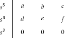
Special Case 1: If the first element of any row of Routh's array becomes zero (other elements of the row are non zero), then it becomes difficult in examining the stability of the system since the terms in the next row becomes infinite. Consider a system whose characteristic equation is given by ![]() . Examine the stability of the system using Routh's array.
. Examine the stability of the system using Routh's array.
Solution: For the given characteristic equation, Routh's array is formed as:
 .
.
Since the first value in the third row of Routh's array is zero, the first value in the fourth row of Routh's array becomes infinite and makes the examination of the stability of the system difficult. There are three methods to solve and investigate the stability of the system.
Method 1: Replace the zero (first element in the third row) with a small positive real number ![]() and continue the evaluation of the array. After completing the array, examine the possibility of occurrence of a sign change using
and continue the evaluation of the array. After completing the array, examine the possibility of occurrence of a sign change using ![]() . Considering the same example, replace the first element of the third row by ε and continue evaluating the array.
. Considering the same example, replace the first element of the third row by ε and continue evaluating the array.
 .
.
Now, for examining the occurrence of a sign change, consider all the elements in the array that has ε in it and apply the limits.
![]()
![]()
Then, replace these values in Routh's array to have a clear idea about the sign changes occurring in the system. The modified Routh's array will be as follows:
 .
.
Since there are two sign changes in the first column of Routh's array i.e., ![]() to
to ![]() and
and ![]() to +1.5, two roots lie in the right half of the s-plane. Hence the system is unstable.
to +1.5, two roots lie in the right half of the s-plane. Hence the system is unstable.
Method 2: In this method, the variable s in the characteristic equation of the system is replaced by the variable ![]() . After rearranging the characteristic equation using the variable, x, Routh's array is formed and then the stability of the system is examined.
. After rearranging the characteristic equation using the variable, x, Routh's array is formed and then the stability of the system is examined.
Consider the same example with the characteristic equation ![]()
Substituting ![]() in the given characteristic equation and rearranging, we obtain the new characteristic equation as follows:
in the given characteristic equation and rearranging, we obtain the new characteristic equation as follows:
![]()
Then Routh's array is formed as:
 .
.
Since there are two sign changes i.e., from 2.33 to −0.429 and from −0.429 to 1 in the first column of Routh's array, two roots lie in the left half of the s-plane. Hence, the system is unstable.
Method 3: When Routh's array has a zero in the first column, we multiply ![]() by a factor
by a factor ![]() where
where ![]() is positive, say
is positive, say ![]() Since
Since ![]() has all zeros of
has all zeros of ![]() and zero at
and zero at ![]() the change of sign in Routh's array of
the change of sign in Routh's array of ![]() will indicate the existence of pseudo- positive roots in
will indicate the existence of pseudo- positive roots in ![]() The following example illustrates this point.
The following example illustrates this point.
Consider the same example with the characteristic equation ![]()
Multiply ![]() by a factor
by a factor ![]() to obtain the new characteristic equation as
to obtain the new characteristic equation as
![]()
Routh array for the modified characteristics equation is
 .
.
 .
.
Since there are two sign changes i.e., from 2 to −1 and from −1 to 9 in the first column of Routh's array, two roots lie in the right half of the s-plane. Hence, the system is unstable.
Example 6.15: The open-loop transfer function of a unity feedback system is ![]() . Find the number of roots that lie in the right half of the s-plane.
. Find the number of roots that lie in the right half of the s-plane.
Solution: Given ![]() and H(s) = 1.
and H(s) = 1.
The characteristic equation is
![]()
or
![]()
Routh's array for the characteristic equation is
 .
.
Since the first value in the third row of Routh's array is zero, the first value in the fourth row of Routh's array becomes infinite. Hence, it is difficult to examine the stability of the system. The new characteristic equation can be obtained by replacing s by ![]() as follows:
as follows:
![]()
Then, Routh's array is formed as:
 .
.
Since there are two sign changes i.e., from 5 to −1.8 and from −1.8 to ![]() in the first column of Routh's array, two poles lie in the right half of the s-plane.
in the first column of Routh's array, two poles lie in the right half of the s-plane.
Example 6.16: Examine whether the system with the following characteristic equation ![]() is stable. Also, find the nature of the roots of the equation.
is stable. Also, find the nature of the roots of the equation.
Solution: Routh's array for the given characteristic equation is tabulated as follows:
 .
.
When a zero comes in the first column of Routh's array, the method of testing the stability is as follows:
Substituting ![]() in the characteristic equation, we obtain
in the characteristic equation, we obtain
![]()
![]()
![]()
Routh's array for the above equation is tabulated as follows:
 .
.
There are two sign changes i.e., from 1 to −1 and from −1 to 2 exist in the first column of Routh's array. Therefore, there are two roots in the right half of the s-plane. Hence, the system is unstable.
To find the Number of Roots in the Left Half of the s-Plane
To find the number of roots existing in the left half of the s-plane, replace s with -s in the given characteristic equation
![]()
Routh's array for the above equation is tabulated as
 .
.
When a zero comes in the first column of Routh's array, the method of testing the stability is as follows:
Substituting ![]() in the characteristic equation, we obtain
in the characteristic equation, we obtain
![]()
Routh's array for the above equation is tabulated as
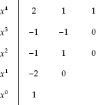 .
.
There are two sign changes i.e., from 2 to −1 and −2 to 1 in the first column of Routh's array. Therefore, there are two roots in the left half of the s-plane.
It is already known that there are two roots in the right half of the s-plane. There are totally four roots for the above characteristic equation. Therefore, there is no root on the imaginary axis. The result is that the system is unstable.
Example 6.17: The characteristic equation of the system is given by ![]() Investigate the stability of the system using Routh's array.
Investigate the stability of the system using Routh's array.
Solution: For the given characteristic equation ![]() Routh's array is formed as:
Routh's array is formed as:
 .
.
Since the first value in the third row of Routh's array is zero, the first value in the fourth row of Routh's array becomes infinite. Hence, the above characteristic equation can be investigated for the stability of the system using the following two methods tabulated below.

Since there are two sign changes in the first column of the modified Routh's array obtained from both the methods, two poles of the system are located in the right half of the s-plane. Hence, the system is unstable.
Example 6.18: Investigate the stability of a system using Routh's criterion for the characteristic equation of a system given by ![]()
Solution: Given the characteristic equation of the system is
![]()
Then, Routh's array is formed as:
 .
.
Since the first value in the third row of Routh's array is zero, the first value in the fourth row of Routh's array becomes infinite.
The above characteristic equation can be investigated for the stability of the system using the following two methods tabulated below.

Since there are two sign changes in the first column of the modified Routh's arrays obtained from both the methods, two poles of the system are located in the right half of the s-plane. Hence, the system is unstable.
Special Case 2: If all the elements of any row of Routh's array become zero or if all the elements of (n−1)th row is an integral multiple of nth row, then it becomes difficult to examine the stability of the system as determining the terms in the next row becomes difficult.
Consider a system whose characteristic equation is given by ![]()
![]() .
.
Examine the stability of the system using Routh's array.
Solution: For the characteristic equation ![]() , Routh's array is formed as:
, Routh's array is formed as:
 .
.
Since all the elements in the third row of Routh's array is zero, it becomes difficult to determine the values of the element present in the next row and makes the examination of the stability of the system difficult.
Solution for Such Cases Consider a Routh's array in which all the elements of third row are zero as given below:
 .
.
Elimination Procedure to overcome the Difficulty: The steps involved in eliminating the above-mentioned difficulty are listed below:
- An auxiliary equation, A(s) is formed with the coefficients present in the row i.e., just above the row of zeros. The auxiliary equation is formed with the alternate powers of s starting from the power indicated against it. For the given example, the auxiliary equation is given by
 .
. - The first-order derivative of the auxiliary equation with respect to s is determined, which is given by
 .
. - The coefficients of
 is used to replace the row of zeros. Hence, now Routh's array is given as follows:
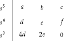 .
. - Now Routh's array is completed with the help of these new coefficients and the stability of the system is examined.
Importance of an Auxiliary Equation: ![]() : Auxiliary equation is a part of the original characteristic equation i.e., the roots of the auxiliary equation belong to the original characteristic equation also. In addition, the roots of the auxiliary equation are the most dominant roots of the original characteristic equation. The roots of the auxiliary equation are called the dominant roots since it decides the stability of the system.
: Auxiliary equation is a part of the original characteristic equation i.e., the roots of the auxiliary equation belong to the original characteristic equation also. In addition, the roots of the auxiliary equation are the most dominant roots of the original characteristic equation. The roots of the auxiliary equation are called the dominant roots since it decides the stability of the system.
Hence, the stability of the system can be predicted easily by determining the roots of the auxiliary equation ![]() (dominant roots) rather than determining all the roots of the characteristic equation. The remaining roots of the characteristic equation do not play any significant role in the stability analysis.
(dominant roots) rather than determining all the roots of the characteristic equation. The remaining roots of the characteristic equation do not play any significant role in the stability analysis.
For example, if the order of the characteristic equation ![]() is n and the order of auxiliary equation
is n and the order of auxiliary equation ![]() is m, then the number of roots that play a significant role in the stability analysis of the system is given by m. Hence,
is m, then the number of roots that play a significant role in the stability analysis of the system is given by m. Hence,
Number of dominant roots = m.
Number of non-dominant roots = ![]() .
.
On completion of Routh's array with the help of auxiliary equation, two suggestions over the stability are as follows:
- If there is any sign change in the first column of the modified Routh's array, then we can conclude that the system is unstable since some of the roots lie in the right side of the s-plane.
- If there is no sign change in the first column of the modified Routh's array, we cannot suggest that the system is stable. Only after finding the roots of the auxiliary equation (dominant roots), we can find the stability of the system.
The different location of roots of auxiliary equation in the s-plane and the corresponding nature of stability of the system are shown in Table 6.4.
Example 6.19: The characteristic equation of a system is given by s3 + 10s2 + 50s + 500 = 0. Investigate the stability of the system using Routh's array.
Solution: For the characteristic equation of the system ![]() , Routh's array is formed as follows:
, Routh's array is formed as follows:
 .
.
As all the elements in the third row of Routh's array are zero, it becomes difficult to determine the values of the elements present in the next row. This makes the examination of the stability of the system difficult. To eliminate this difficulty, the following steps are carried out:
Step 1: Auxiliary equation of the system is given by ![]() .
.
Step 2: First-order derivative of the auxiliary equation is given by ![]() .
.
Step 3: The coefficient of the first-order derivative of the auxiliary equation is used to replace the row of zeros. The modified Routh's array is given by
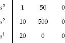 .
.
Step 4: With the help of new coefficients, the complete Routh's array is formed as:
 .
.
Although there is no sign change in the first column of Routh's array, the system cannot be suggested as a stable system. For suggesting the stability of the system, the roots of the auxiliary equation A(s) are to be determined.
Upon solving A(s) = 0, i.e., 10s2 + 500 = 0, we obtain ![]() , which are the dominant roots of the given characteristic equation. The given system is marginally stable because the dominant roots are on the imaginary axis of the s-plane.
, which are the dominant roots of the given characteristic equation. The given system is marginally stable because the dominant roots are on the imaginary axis of the s-plane.
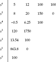
Example 6.20: The characteristic polynomial of a system is ![]() Check whether the system is stable, marginally stable, unstable or oscillatory.
Check whether the system is stable, marginally stable, unstable or oscillatory.
Solution: For the characteristic polynomial of a system ![]() , Routh's array is formed as:
, Routh's array is formed as:
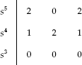 .
.
Since all the elements in the third row are zero, the auxiliary equation A(s) is formed as A(s) = s4 + 2s2 + 1. i.e., A(s) = (s2 + 1 )2 = 0.
The dominant roots of the characteristics equation (or) roots of auxiliary equation are j, j, −j, −j.
Since repeated roots exist on the imaginary axis, the given system is unstable.
Example 6.21: The characteristic equation of the system is given by ![]() Investigate the stability of the system using Routh's array.
Investigate the stability of the system using Routh's array.
Solution: For the characteristic equation of the system ![]() Routh's array is formed as:
Routh's array is formed as:
 .
.
Here, all the elements in the fifth row of Routh's array are zero. Hence, the following steps are carried out to determine the values of the elements present in the next row.
Step 1: Auxiliary equation for the system is given by ![]() .
.
Step 2: First-order derivative of the auxiliary equation is given by ![]() .
.
Step 3: The coefficient of the first-order derivative of the auxiliary equation is used to replace the row of zeros. The modified Routh's array is given by
 .
.
Step 4: The complete Routh's array is formed with the help of new coefficients and is given by
 .
.
Although there is no sign change in the first column of Routh's array, the system cannot be suggested as a stable system. For suggesting the stability of the system, the roots of the auxiliary equation ![]() are to be determined.
are to be determined.
Upon solving, A(s) = 0, i.e., ![]() we obtain
we obtain ![]() , which are the dominant roots of the given characteristic equation obtained using auxiliary equation.
, which are the dominant roots of the given characteristic equation obtained using auxiliary equation.
The given system is marginally stable because the dominant roots are on the imaginary axis of the s-plane.
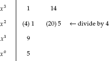
Example 6.22: For the characteristic equation ![]() find the number of roots which lie in the right half and the left half of the s-plane.
find the number of roots which lie in the right half and the left half of the s-plane.
Solution:
- To find the number of roots in the right of the s-plane
For the characteristic equation of the system,
 , Routh's array is formed as:
 .
.In the above Routh's array, all the elements in the fourth row are zero. Therefore, the auxiliary equation for the system is given by

i.e.,

The coefficient of the first-order derivative of the auxiliary equation is used to replace the row of zeros. The modified Routh's array is formed as:
 .
.As there is only one sign change i.e., from 4 to −1.5 in the first column, only one root falls in the right half of the s-plane.
- To find the number of roots in the left half of the s-plane
In order to find the number of roots in the left half of the s-plane,
 is obtained and corresponding Routh's array is formed. The number of sign changes indicates the number of roots in the left half of the s-plane. Therefore,
Routh's array is formed as:
 .
.In the above Routh's array, all the elements in the third row are zero. Therefore, the auxiliary equation of the system is

i.e.,

The coefficient of the first order derivative of the auxiliary equation is used to replace the row of zeros. The modified Routh's array is formed as:
 .
.There are three sign changes (from 1 to −1, −1 to 1 and 4 to −1.5) in the first column of Routh's array. Hence, there are three roots in the left half of the s-plane. We have already seen that there is one root in the right half of the s-plane. Since the order of the equation is six, there are totally six roots for the above characteristic equation. Therefore, the remaining two roots lie on the imaginary axis.
6.11.3 Applications of Routh's Criterion
- Relative Stability Analysis: Routh's criterion helps in determining the relative stability of the system about a particular line
 . Axis of the s-plane is shifted by –
 and then Routh's array is formed by substituting
  in the characteristic equation. The number of sign changes in the first column of the new Routh's array is equal to the number of roots located on the right side of the vertical line
The shifting of the s-plane by –
 is clearly shown in Fig. 6.13.
Fig. 6.13 ∣ Relative stability
- To Determine the Range of Values of K: Consider a practical system whose block diagram is shown in Fig. 6.14. The range of gain, K could be determined using Routh's array.

Fig. 6.14 ∣ Block diagram of a control system
The closed-loop transfer function of the system shown in Fig. 6.14 is given by

Hence, the characteristic equation of the system is given by

The stability of the system or the location of roots of the characteristic equation (poles of the system) depends on the proper selection of value of gain, K. To determine the range of K, following steps are used:
- Routh's array is completed in terms of gain value K.
- Range of values of K is determined such that the sign of all values present in the first column of Routh's array remains same.
Since the stability of the system depends on the value of the gain K, the system is conditionally stable.
6.11.4 Advantages of Routh's Criterion
The advantages of Routh's criterion of examining the stability for the given system are as follows:
- It does not require solving the characteristic equation to examine the stability of the system.
- It is less time-consuming method as there is no requirement of finding the determinant values.
- Relative stability of the system is examined.
- The value of system gain for which the system has sustained oscillations could be determined and hence the frequency of oscillations can also be determined.
- Helps in determining the range of system gain for which the system is stable.
6.11.5 Limitations of Routh's Criterion
The following are the limitations of Routh's criterion:
- Stability of the system can be examined if and only if the characteristic equation has real coefficients.
- There is difficulty in providing the exact location of the closed-loop poles.
- It does not suggest any method for stabilizing the unstable system.
- It is applicable only to LTI systems.
Example 6.23: The characteristic equation of the system is given by F(s) = s(s2 + s + 1) (s + 4) + K = 0. Investigate the range of values of gain, K, using Routh's array for the system to be stable.
Solution: The characteristic equation for the system is
![]()
Then, Routh's array is formed as:
 .
.
The condition for the system to be stable is that the sign of all the values in the first column should be the same.
Hence, ![]() ,
, ![]()
Therefore, the range of values of gain, K for the system to be stable is ![]()
Example 6.24: A closed-loop system described by the transfer function is given by  is stable. Determine the constraints on
 ![]() .
.
Solution: The characteristic equation is ![]()
Routh's array is formed as follows:
 .
.
For the system to be stable, ![]()
Thus, ![]()
Example 6.25: The characteristic equation of the system is given by s4 + s3 + 3Ks2 + (K + 2)s + 4 = 0. Examine the range of values of gain K using Routh's array for the system to be stable.
Solution: The characteristic equation given for the system is
![]()
Then, Routh's array is formed as:
 .
.
The condition for the system to be stable is that there should not be any sign change in the first column of Routh's array.
Hence, ![]() ,
, ![]()
From the first condition, we obtain
![]()
From the second condition, we obtain
K2 + K − 4 > 0 i.e., K > 1.5615 and K > −2.5615
Therefore, the range of values of gain K for the system to be stable is
![]()
Example 6.26: The feedback control system is shown in Fig. E6.26. Find the range of values of ![]() for the system to be stable.
for the system to be stable.

Fig. E6.26
Solution: From the block diagram, the transfer function is

where 
and ![]()
The characteristic equation is given by
![]()

or ![]()
or ![]()
Routh's array is formed as:
 .
.
For the system to be stable, ![]() and
and ![]() . This gives
. This gives ![]()
For ![]() the system will remain stable.
the system will remain stable.
Example 6.27: For the function F(s) = s4 + Ks3 + (K + 4)s2 + (K + 3)s + 4 = 0, find the real value of K so that the system is just oscillatory.
Solution:
 .
.
From the above Routh's array, it is clear that ![]() .
.
Also, ![]()
and ![]()
![]()
The condition ![]() and
and ![]() imposes that
imposes that ![]() is positive. Hence,
is positive. Hence, ![]()
![]() imposes that
imposes that ![]()
![]() imposes that
imposes that ![]()
Hence, ![]() for absolute stability.
for absolute stability.
At ![]() , the system oscillates.
, the system oscillates.
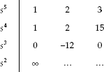
Example 6.28: Determine the positive values of K and ![]() so that the system shown in the Fig. E6.28 oscillates at a frequency of 2 rad/sec,
so that the system shown in the Fig. E6.28 oscillates at a frequency of 2 rad/sec,

Fig. E6.28
Solution: The characteristic equation is given by
![]()
![]()
![]()
Routh's array is formed as:
 .
.
For the system to have oscillations,
![]()
or ![]() (1)
(1)
Then, we have ![]() (2)
(2)
Given ![]() rad/sec, substituting s = jω,
rad/sec, substituting s = jω,
![]()
Thus, ![]()
Upon solving Equations (1) and (2), we obtain ![]() .
.
Example 6.29: Determine the range of values of K(K > 0) such that the characteristic equation s3 + 3(K + 1)s2 + (7K + 5)s + (4K + 7) = 0 has roots more negative than ![]() .
.
Solution: Given the characteristic equation ![]() . To find the roots more negative than
. To find the roots more negative than ![]() , replace s with
, replace s with ![]() . Then, the new characteristic equation becomes
. Then, the new characteristic equation becomes
![]() .
.
Simplifying, we obtain
![]()
For the new characteristic equation, Routh's array is formed as:
 .
.
Here, ![]() and
and ![]() i.e.,
i.e., ![]()
Therefore, the range of values of K is ![]() .
.
Example 6.30: The open-loop transfer function of the system is given by  , which has a unity feedback system.
- Determine the relation between K and T so that the system is stable.
- Determine the relation between K and T if all the roots of characteristic equation obtained for the same system as given above have to lie on the left side of the line
 in the s-plane.
Solution:
- The characteristic equation of the system with unity feedback is given by


Therefore, Routh's array is formed as:
 .
.The condition for the system to be stable is that there should not be any sign change in the first column of Routh's array. Therefore,

The relation between the gain values of K and T for the system to be stable is given by
 and its pictorial representation is shown in Fig. E6.30(a).
Fig. E6.30(a)
- The stability condition can be determined by estimating the roots that lie on the right side of the line, s = −1. The following steps are carried out:
- Replace s by
 in the characteristic equation and determine the new characteristic equation:

Therefore,

- Routh's array is formed as:
 .
.
The condition for the system to be stable is that there should not be any sign change in the first column of Routh's array.
Hence,
 and
and 
From the first condition, we obtain

From the second condition, we obtain

The relation between the gain values K and T for the system to be stable is given by the above two relations and its pictorial representation is shown in Fig. E6.30(b).

Fig. E6.30(b)
- Replace s by
Example 6.31 The open-loop transfer function of a unity feedback control system is given by  . Examine the stability of the system using Routh's array.
Solution: The characteristic equation of the unity feedback control system is given by
![]()
Therefore, 
![]()
Here, ![]()
Considering the first three terms of the above expression, the characteristic equation is

Then, Routh's array is formed as:
 .
.
The condition for the system to be stable is that there should not be any sign change in the first column of Routh's array.
Hence, ![]() and
and ![]()
Thus, for all values of ![]() , the system remains stable.
, the system remains stable.
Example 6.32: The open-loop transfer function of a unity feedback control system is given by  .
.
- Examine the range of values of gain K, using Routh's table for the system to be stable.
- Also, determine the value of K which causes sustained oscillation in the system and then determine the frequency of sustained oscillations.
Solution:
- The characteristic equation of the unity feedback control system is given by


Then, Routh's array is formed as:
 .
.The condition for the system to be stable is that there should not be any sign change in the first column of Routh's array. Hence,
 therefore,
 therefore,
Thus, the range of values of gain
 for which the system remains stable is
- To have a sustained oscillations in the system, all the values in any row in Routh's array must be zero. Therefore, in the fourth row, if we substitute a proper value of K, we can make all the elements in that row to be zero. Hence, for K = 666.25, Routh's array is
 .
.Hence, the system has sustained oscillations for the value of K = 666.25. To determine the frequency of the sustained oscillations, the auxiliary equation A(s) is solved for the roots.
The auxiliary equation for the above Routh's array is given by

Upon solving, we get

Hence, the frequency of the sustained oscillations is 4.062 rad/sec.
Example 6.33: The block diagram representation of a unity feedback control system is shown in Fig. E6.33. Determine the range of values of gain K using Routh's array for the system to be stable.

Fig. E6.33
Solution: The characteristic equation of the unity feedback control system is given:
![]()
![]()
![]()
Then, Routh's array is formed as:
 .
.
The condition for the system to be stable is that there should not be any sign change in the first column of Routh's array. Hence,


Therefore,

The range of values of gain for which the system remains stable is
 .
.
Review Questions
- Define stability?
- What is BIBO stability?
- Define asymptotic stability of a system.
- Distinguish between absolute stability and relative stability.
- Explain the concept of stability of feedback control system.
- Write down the general form of the characteristic equation of a closed-loop system.
- Write down the characteristic equation for

- What is Hurwitz criterion?
- What are the conditions required for a system to be stable? How does Routh–Hurwitz criterion help in deciding a stable system?
- What are the difficulties faced while applying Routh–Hurwitz criterion?
- What are the two special cases in applying Routh–Hurwitz criteria?
- Is Routh–Hurwitz criterion applicable if
- the characteristic equation is non-algebraic?
- a few of the coefficients are not real?
- Using Routh's criterion, determine the stability of the system represented by the characteristic equation:
 Comment on the locations of the roots of the characteristic equation.
 - Define dominant poles and zeros.
- Explain Routh's Hurwitz stability criterion.
- The characteristic equation of a system is given by
 . Using Routh–Hurwitz criterion, find out whether the system is stable or not. Also, find the number of roots lying in the left half of the s-plane.
 - Check whether the characteristic equation
 represents a stable system or not.
 - For the characteristic equation
 , find the number of roots lying to the left half of the vertical line through −1.
 - Investigate the stability using Routh–Hurwitz stability criterion, for the closed-loop system whose characteristic equation is
 .
. - Check the stability of the following system whose characteristic equations is
 .
. - By means of Routh–Hurwitz stability criterion, determine the stability of the system with the characteristic equation
 Also determine the number of roots of the equation that are in the right half of the s-plane.
 - Apply Routh's criteria to determine the number of roots in the positive half of the s-plane for the polynomial
 .
. - The characteristic equation of a system is given by
 Determine the number of roots in the left and right half of the s-plane.
 - Examine the stability of the system whose characteristic equation is given by

- Investigate the characteristic equation for the distribution of its roots:

- Consider the unity feedback system with the open-loop transfer function:
 Is this system stable?
 - Study the stability of a feedback control system whose loop transfer function is

- The characteristic equation of a control system is
 . Determine the range of
  for which the system is stable.
 - The characteristic equation of a system is
 Find the range of values of
  for which the system will be stable.
 - Determine the range of
 such that the feedback system with characteristic equation
  is stable.
 - For the system whose characteristic equation is
 find the range of values of
  for the system to be stable.
 - The open-loop transfer function of a unity feedback control system is given by
 where
where  and
and  are both positive. Represent the region of stability in the parameter plane
  .
. - A system oscillates with a frequency
 if it has poles at
  and no poles in the right half of the s-plane. Determine the values of
  and
and  so that the system whose open-loop transfer function
  oscillates at frequency 2 rad/sec.
 - The closed-loop transfer function of a system is given by
 Determine the range of
  for which the system is stable.
 - Obtain the value of
 for the system whose characteristic equation given by
  is to be stable.
 - Determine the range of
 such that the feedback system having the characteristic equation
  is stable.
 - Find the range of
 for stability of unity feedback control system having open-loop transfer function as
  .
. - The characteristic equation for a feedback control system is given by

- Find the range of
 for stability.
 - What is the frequency in rad/sec at which the system will oscillate?
- How many roots of the characteristic equation lie in the right half of the s-plane when

- Find the range of
- Investigate the stability condition for the system with the characteristic equation F(s) = (s − 1)2 (s + 2) = 0.
- The open-loop transfer function of a unity feedback system is
 .
.
Determine the range of values of K for which the system is stable.