3
BLOCK DIAGRAM REDUCTION TECHNIQUES
3.1 Introduction to Block Diagram
A block diagram is a diagrammatic representation of the cause-and-effect relationship between the input and output of a physical system represented by the flow of signals. It gives the relationship that exists between various components of a system. The open-loop and the closed-loop systems discussed in Chapters 1 and 2 can be represented by using the block diagram reduction techniques.
3.2 Open-Loop and Closed-Loop Systems Using Block Diagram
A system that cannot change its output in accordance to the change in input is known as a open-loop system. Such an open-loop system can be represented by using a block diagram as shown in Fig. 3.1.

Fig. 3.1 ∣ Open-loop system
A system that can change its output in accordance with change in input is known as a closed-loop system. This can be implemented by introducing a feedback path in a open-loop system and manipulating the input that is applied to the system. Such a closed-loop system can be represented by using a block diagram shown in Fig. 3.2.

Fig. 3.2 ∣ Closed-loop system
3.2.1 Advantages of Block Diagram Representation
The advantages of block diagram representation are:
- It facilitates easier representation of complex systems.
- Calculation of transfer function by block diagram reduction techniques is easy.
- Performance analysis of a complex system is simplified by determining its transfer function.
- It facilitates easier access of individual elements in a system that is represented by a block diagram.
- It facilitates visualization of operation of the whole system by the flow of signals.
3.2.2 Disadvantages of Block Diagram Representation
The disadvantages of block diagram representation are:
- It is difficult to determine the actual composition of individual elements in a system.
- Representation of a system using block diagram is not unique.
- The main source of signal flow cannot be represented definitely in a block diagram.
3.3 Block Diagram Representation of Electrical System
The flow chart to represent any electrical system by means of a block diagram is shown in Fig. 3.3.

Fig. 3.3 ∣ Flow chart for representing an electrical system by a block diagram
Example 3.1: Represent the electrical circuit shown in Fig. E3.1(a) by a block diagram.

Fig. E3.1(a)
Solution: The current flowing through the electrical circuit shown in Fig. E3.1(a) is given by
![]() (1)
(1)
The output voltage across the capacitor C is determined by
![]() (2)
(2)
Individual block diagrams representing each of the above equations can be determined by examining the input and output of the respective equations. Then, these individual block diagrams can be combined in an appropriate way to represent the given electrical circuit.
To Determine the Individual Block Diagrams:
For Eqn. (1):
Taking Laplace transform of Eqn. (1), we obtain
![]() (3)
(3)
where the inputs are Vi (s) and Vo (s) and the output is I(s). Hence, the block diagram for the above equation is shown in Fig. E3.1(b).

Fig. E3.1(b)
For Eqn. (2):
Taking Laplace transform of Eqn. (2), we obtain
![]() (4)
(4)
where the input is ![]() and the output is
and the output is ![]() . Hence, the block diagram for the above equation is shown in Fig. E3.1(c).
. Hence, the block diagram for the above equation is shown in Fig. E3.1(c).

Fig. E3.1(c)
Thus, the overall block diagram for the given electrical circuit is obtained by interconnecting the block diagrams shown in Figs. E3.1(b) and (c). The overall block diagram of the given electrical circuit is shown in Fig. E3.1(d).

Fig. E3.1(d)
Example 3.2: Represent the electrical circuit shown in Fig. E3.2(a) by a block diagram.

Fig. E3.2(a)
Solution: Resistors R1, R2, R3 and inductances L1, L2 are in a series path. Capacitors C1, C2 and C3 are in a shunt path. The loop currents indicated in the given electrical circuit are ![]() ,
, ![]() and
and ![]() . The node voltages for the given electrical circuit are
. The node voltages for the given electrical circuit are ![]() and
and ![]() . The input voltage is
. The input voltage is ![]() and the output voltage across the capacitor
and the output voltage across the capacitor ![]() is
is ![]() .
.
The current flowing through each element in series path is determined by using the node voltages.
The same current flows through resistor R1 and inductor L1. Hence, using the node voltages ![]() and
and ![]() , the current
, the current ![]() can be obtained as
can be obtained as
![]() (1)
(1)
Similarly, the current flowing through resistor R2 and inductor L2 can be obtained by using the node voltages ![]() and
and ![]() as
as
![]() (2)
(2)
The current flowing through resistor R3 can be obtained by using the node voltages ![]() and
and ![]() as
as
![]() (3)
(3)
The voltages across each element present in the shunt path can be determined by using the loop currents.
The voltage ![]() across the capacitor C1 is given by
across the capacitor C1 is given by
![]() (4)
(4)
The voltage ![]() across the capacitor C2 is given by
across the capacitor C2 is given by
![]() (5)
(5)
The voltage ![]() across the capacitor C3 is given by
across the capacitor C3 is given by
![]() (6)
(6)
Individual block diagrams representing each of the above equations can be determined by examining the input and output of the respective equations. Then, these individual block diagrams can be combined in an appropriate way to represent the given electrical circuit.
To determine the individual block diagrams:
For Eqn. (1):
Taking Laplace transform of Eqn. (1), we obtain
![]()
![]() (7)
(7)
where the inputs are ![]() and
and ![]() and the output is
and the output is ![]() . Hence, the block diagram for the above equation is shown in Fig. E3.2(b).
. Hence, the block diagram for the above equation is shown in Fig. E3.2(b).

Fig. E3.2(b)
For Eqn. (2):
Taking Laplace transform of Eqn. (2), we obtain
![]()
![]() (8)
(8)
where the inputs are ![]() and
and ![]() and the output is
and the output is ![]() . Hence, the block diagram for the above equation is shown in Fig. E3.2(c).
. Hence, the block diagram for the above equation is shown in Fig. E3.2(c).

Fig. E3.2(c)
For Eqn. (3):
Taking Laplace transform of Eqn. (3), we obtain
![]()
Therefore, ![]() (9)
(9)
where the inputs are ![]() and
and ![]() and the output is
and the output is ![]() . Hence, the block diagram for the above equation is shown in Fig. E3.2(d).
. Hence, the block diagram for the above equation is shown in Fig. E3.2(d).

Fig. E3.2(d)
For Eqn. (4):
Taking Laplace transform of Eqn. (4), we obtain
![]() (10)
(10)
where the inputs are ![]() and
and ![]() and the output is
and the output is ![]() . Hence, the block diagram for the above equation is shown in Fig. E3.2(e).
. Hence, the block diagram for the above equation is shown in Fig. E3.2(e).

Fig. E3.2(e)
For Eqn. (5):
Taking Laplace transform of Eqn. (5), we obtain
![]() (11)
(11)
where the inputs are ![]() and
and ![]() and the output is
and the output is ![]() . Hence, the block diagram for the above equation is shown in Fig. E3.2(f).
. Hence, the block diagram for the above equation is shown in Fig. E3.2(f).

Fig. E3.2(f)
For Eqn. (6):
Taking Laplace transform of Eqn. (6), we obtain
![]() (12)
(12)
where the input is ![]() and the output is
and the output is ![]() . Hence, the block diagram for the above equation is shown in Fig. E3.2(g).
. Hence, the block diagram for the above equation is shown in Fig. E3.2(g).
Fig. E3.2(g)
Hence, the overall block diagram for the given electrical circuit is obtained by interconnecting the block diagrams shown in Figs. E3.2(b) through (g). The overall block diagram of the given electrical circuit is shown in Fig. E3.2(h).

Fig. E3.2(h)
Example 3.3: Represent the armature-controlled DC motor shown in Fig. E3.3(a) by a block diagram.
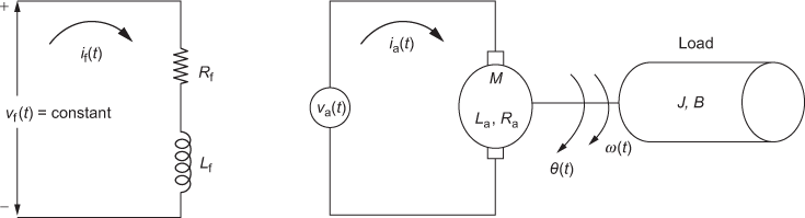
Fig. E3.3(a)
Solution: The equivalent electrical circuit of armature circuit is shown in Fig. E3.3(b).

Fig. E3.3(b)
Applying Kirchhoff's voltage law, the differential equation can be obtained as
![]() (1)
(1)
The relationship between the torque applied to the load and armature current is given by
![]() (2)
(2)
The equivalent rotational mechanical system of the load connected to DC motor is shown in Fig. E3.3(c).

Fig. E3.3(c)
Using D'Alembert's principle, we have
![]() (3)
(3)
where ![]() is the angular velocity.
is the angular velocity.
The relation between back emf eb(t) and angular velocity ω(t) is given by
![]() (4)
(4)
The equation relating the angular velocity and angular displacement ![]() is given by
is given by
![]() (5)
(5)
Individual block diagrams representing each of the above equations can be determined by examining the input and output of the respective equations. Then, these individual block diagrams can be combined in an appropriate way to represent the armature-controlled DC motor.
To determine the individual block diagrams:
For Eqn. (1):
Taking Laplace transform of Eqn. (1), we obtain
![]() (6)
(6)
where the inputs are ![]() and
and ![]() and the output is
and the output is ![]() . Hence, Eqn. (6) can be rewritten as
. Hence, Eqn. (6) can be rewritten as
 (7)
(7)
Hence, the block diagram for the above equation is shown in Fig. E3.3(d).

Fig. E3.3(d)
For Eqn. (2):
Taking Laplace transform of Eqn. (2), we obtain
![]() (8)
(8)
where the input is ![]() and the output is
and the output is ![]() . Hence, the block diagram for the above equation is shown in Fig. E3.3(e).
. Hence, the block diagram for the above equation is shown in Fig. E3.3(e).
Fig. E3.3(e)
For Eqn. (3):
Taking Laplace transform of Eqn. (3), we obtain
![]() (9)
(9)
where the input is ![]() and the output is
and the output is ![]() . Hence Eqn. (9) can be rewritten as
. Hence Eqn. (9) can be rewritten as
![]() (10)
(10)
Thus, the block diagram for Eqn. (10) is shown in Fig. E3.3(f).

Fig. E3.3(f)
For Eqn. (4):
Taking Laplace transform of Eqn. (4), we obtain
![]() (11)
(11)
where the input is ![]() and the output is
and the output is ![]() . Hence, the block diagram for the above equation is shown in Fig. E3.3(g).
. Hence, the block diagram for the above equation is shown in Fig. E3.3(g).
Fig. E3.3(g)
For Eqn. (5):
Taking Laplace transform of Eqn. (5), we obtain
![]() (12)
(12)
where the input is ![]() and the output is
and the output is ![]() . Hence, Eqn. (12) can be rewritten as
. Hence, Eqn. (12) can be rewritten as
![]() (13)
(13)
Hence, the block diagram for the above equation is shown in Fig. E3.3(h).

Fig. E3.3(h)
Hence, the overall block diagram of armature-controlled DC motor is obtained by interconnecting the block diagrams shown in Fig. E3.3(d) through (h). The overall block diagram of the armature-controlled DC motor is shown in Fig. E3.3(i).

Fig. E3.3(i)
Example 3.4: Represent the field-controlled DC motor shown in Fig. E3.4(a) by a block diagram.

Fig. E3.4(a)
Solution: The equivalent circuit of electrical circuit is shown in Fig. E3.4(b).

Fig. E3.4(b)
Applying Kirchhoff's voltage law, we have
![]() (1)
(1)
The relationship between the torque applied to the load and the field current is given by
![]() (2)
(2)
The equivalent rotational mechanical system of the load connected to a DC motor is shown in Fig. E3.4(c).

Fig. E3.4(c)
Using D'Alembert's principle, we have
![]() (3)
(3)
Individual block diagrams representing each of the above equations can be determined by examining the input and output of the respective equations. Then, these individual block diagrams can be combined in an appropriate way to represent the field-controlled DC motor.
To determine the individual block diagrams:
For Eqn. (1):
Taking Laplace transform of Eqn. (1), we obtain
![]() (4)
(4)
In the above equation, the input is ![]() and the output is
and the output is ![]() . Hence, the above equation can be rewritten as
. Hence, the above equation can be rewritten as
![]() (5)
(5)
The block diagram representing the above equation is shown in Fig. E3.4(d).

Fig. E3.4(d)
For Eqn. (2):
Taking Laplace transform of Eqn. (2), we obtain
![]() (6)
(6)
In the above equation, ![]() is the input and
is the input and ![]() is the output. Hence, the block diagram for the above equation is shown in Fig. E3.4(e).
is the output. Hence, the block diagram for the above equation is shown in Fig. E3.4(e).
Fig. E3.4(e)
For Eqn. (3):
Taking Laplace transform of Eqn. (3), we obtain
![]() (7)
(7)
where ![]() is the input and
is the input and ![]() is the output. Hence, the above equation can be rewritten as
is the output. Hence, the above equation can be rewritten as
![]() (8)
(8)
The block diagram representing the above equation is shown in Fig. E3.4(f).
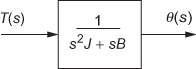
Fig. E3.4(f)
Hence, the overall block diagram of field-controlled DC motor is obtained by interconnecting the block diagrams shown in Figs. E3.4(d) through (f). The overall block diagram of the field-controlled DC motor is shown in Fig. E3.4(g).

Fig. E3.4(g) ∣ Block diagram of field-controlled DC motor
3.4 Block Diagram Reduction
3.4.1 Need for Block Diagram Reduction
In any complex real-time system, many individual sub-systems exist which can be represented by means of individual blocks. The individual blocks of each sub-system shown in Fig. 3.4 are combined to form the block diagram for the system. These individual blocks contain the transfer function of each sub-system.

Fig. 3.4 ∣ Block diagram of complex system
After applying certain rules to the block diagram shown in Fig. 3.4, the complex block diagram can be reduced to a simpler one as shown in Fig. 3.5. Thus, from the reduced form of the block diagram, the transfer function of the complex system can be determined.

Fig. 3.5 ∣ Simplified block diagram
3.4.2 Block Diagram Algebra
Before knowing the rules in reducing the complex block diagram to a simple block diagram, it is necessary to know some terminologies related to the block diagram. Consider a simple block diagram as shown in Fig. 3.6.

Fig. 3.6 ∣ Block diagram
Block
The individual elements of a system can be represented by using blocks, which processes the input signal applied to it and produces an output. The blocks can either be in the forward path or in the feedback path. The blocks for the given block diagram are represented by dotted lines as shown in Fig. 3.7.

Fig. 3.7 ∣ Blocks in the block diagram
Input Signal
A solid line with an arrow at the end pointing towards any block/summing point in the block diagram representation of a system is known as an input signal. A schematic diagram representing one of the input signals is represented by dotted lines in Fig. 3.8.

Fig. 3.8 ∣ Input signal
Forward Path
The flow of signal from the input to output represents the forward path. The representation of the forward path for the block diagram shown in Fig. 3.6 is represented by dotted lines in Fig. 3.9.

Fig. 3.9 ∣ Forward path
Feedback Path
The flow of signal from the output to input represents the feedback path. The representation of the feedback path for the block diagram shown in Fig. 3.6 is indicated by dotted lines in Fig. 3.10.

Fig. 3.10 ∣ Feedback path
Feedback Signal
The signal in the feedback path is known as the feedback signal. For the block diagram given in Fig. 3.6, the feedback signal is denoted by B(s).
Error Signal
The signal obtained by the algebraic sum/difference of any two signals is known as the error signal. In the block diagram shown in Fig. 3.6, the error signal is represented as E(s), which is the algebraic difference of a source input signal and the feedback signal. The error signal is mathematically expressed as
![]()
Summing Point
A block/an element at which two or more signals are either added or subtracted is known as the summing point. The diagram denoting the summing point for the block diagram given in Fig. 3.6 is represented by dotted lines in Fig. 3.11.

Fig. 3.11 ∣ Summing point
Output Signal
The signal that comes out from each block/summing point in any block diagram representing a system is known as the output signal. In the block diagram shown in Fig. 3.6, the output signals are C(s) and ![]() .
.
Take-Off Point
The point at which a signal is applied to two or more blocks is known as the take-off point. The signal might either be an input signal or an output signal. The take-off point for the block diagram shown in Fig. 3.6 is represented by dotted lines in Fig. 3.12. In this case, the output signal is taken as the regulated output and also given as the input to the block in the feedback path.

Fig. 3.12 ∣ Take-off point
3.4.3 Rules for Block Diagram Reduction
Any complex block diagram representing a system can be reduced to a simple block diagram for determining the transfer function by applying certain rules. The rules that can be used in simplifying the given complex block diagram are as explained below. Proof for the rules is obtained by determining the output of the original block diagram and its equivalent block diagram.
- Cascading the blocks in series:
When there are two or more blocks in series without any take-off/summing point in between them, then the individual transfer function of each block is multiplied to form a single block. The original block diagram and its equivalent block diagram are shown in Figs. 3.13(a) and (b) respectively.

From Eqs. (3.1) and (3.2), it is clear that the output obtained after cascading the blocks in series is similar to the original block diagram output.
- Cascading the blocks in parallel:
When there are two or more blocks in parallel in the forward path, then the individual transfer function of each block is added to form a single block. The original block diagram and its equivalent block diagram are shown in Figs. 3.14(a) and (b).

From Eqs. (3.3) and (3.4), it is clear that the output obtained after cascading the blocks in parallel in the forward path is similar to the original block diagram output.
- Reduction of feedback loop:
When there exists a feedback loop in a system, the feedback loop can be reduced to a single block. The feedback loop can either be negative or positive. The blocks representing the feedback loop and its equivalent block diagram are shown in Figs. 3.15(a) and (b).

From Eqs. (3.5) and (3.6), it is clear that the output obtained after reducing the feedback loop is similar to the original feedback loop output.
- Moving the take-off point after/before a block:
The take-off point that exists between the blocks can be moved either before the block or after the block.
- After a block
The changes to be made in the block diagram in moving the take-off point after the block is shown in Fig. 3.16(b). The original block diagram is shown in Fig. 3.16(a).

From Eqs. (3.7) and (3.8), it is clear that the output obtained after shifting the take-off point after a block is similar to the original block diagram output.
- Before a block
The changes to be made in the block diagram in moving the take-off point before the block is shown in Fig. 3.17(b). The original block diagram is shown in Fig. 3.17(a).

From the above proof, it is clear that the output obtained after shifting the take-off point before a block is similar to the original block diagram output.
- After a block
- Moving the summing point after/before a block:
The summing point that adds/subtracts two or more signals can be moved either after or before a block.
- After a block
The changes to be made in the block diagram in moving the summing point after the block is shown in Fig. 3.18(b). The original block diagram is shown in Fig. 3.18(a).

From Eqs. (3.9) and (3.10), it is clear that the output obtained after shifting the summing point after a block is similar to the original block diagram output.
- Before a block
The changes to be made in the block diagram in moving the summing point before the block is shown in Fig. 3.19(b). The original block diagram is shown in Fig. 3.19(a).
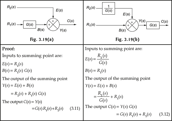
From Eqs. (3.11) and (3.12), it is clear that the output obtained after shifting the summing point before a block is similar to the original block diagram output.
- After a block
- Splitting/joining a summing point:
The summing point that adds/subtracts two or more signals can be split into two summing points, or two summing points can be joined together to have a single summing point.
- Splitting the summing points
A summing point that adds/subtracts three signals can be split into two summing points. The block diagram explaining the concept is shown in Figs. 3.20 (a) and (b).
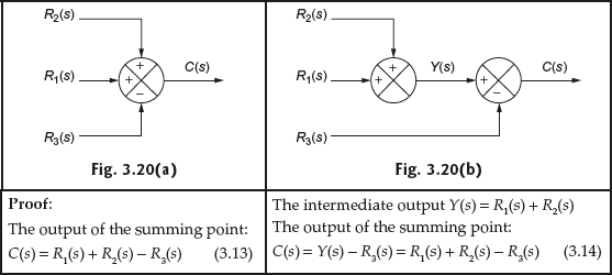
From Eqs. (3.13) and (3.14), it is clear that the output obtained after splitting the summing point is same as the output of the summing point without splitting.
- Joining the summing points
Two or more summing points present in the block diagram can be joined together to form a single summing point. The block diagram explaining the concept is shown in Figs. 3.21(a) and (b).
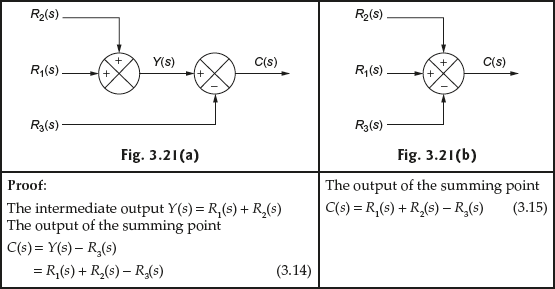
From Eqs. (3.14) and (3.15), it is clear that the output obtained after joining the summing point is same as the output of the summing point without joining.
- Splitting the summing points
- Moving a take-off point after/before a summing point:
The take-off point that exists in the block diagram can be moved after or before a summing point without changing the output of the system. The block diagram explaining the concept is shown in Figs. 3.22 and 3.23.
- After summing point
The changes to be done in the block diagram in shifting the take-off point after a summing point is explained in Figs. 3.22(a) and (b).

From Eqs. (3.16) and (3.17), the output of the take-off point is same even though the take-off point is shifted after a summing point.
- Before summing point
The changes to be done in the block diagram in shifting the take-off point before a summing point is explained in Figs. 3.23(a) and (b).

From Eqs. (3.18) and (3.19), the output of the take-off point is same even though the take-off point is shifted before a summing point.
- After summing point
- Exchanging two or more summing points:
Two or more summing points present in the block diagram can be interchanged without changing the output of the block diagram. The block diagram explaining the concept of exchanging the summing point is shown in Figs. 3.24(a) and (b).

From Eqs. (3.20) and (3.21), it is clear that the output obtained after exchanging the summing points is same as the output of the summing point before exchanging.
3.4.4 Block Diagram Reduction for Complex Systems
The flow chart for reducing the complex block diagram to a simplified block diagram is shown in Fig. 3.25.

Fig. 3.25 ∣ Block diagram reduction flow chart
Example 3.5: For the block diagram of the system shown in Fig. E3.5(a), determine the transfer function using block diagram reduction technique.
Fig. E3.5(a)
Solution:
Step 1:The summing point three input signals as represented by dotted lines in Fig. E3.5(b) can be separated by having the feedback signal separately and others separately. The resultant block diagram is shown in Fig. E3.5(c).

Fig. E3.5(b)
Step 2:The feedback path as represented by dotted lines in Fig. E3.5(c) can be reduced to a single block as shown by dotted lines in Fig. E3.5(d).

Fig. E3.5(c)
Step 3:Now, there exist two cases. One, the take-off point from the signal R(s) can be moved after summing point and the other is the summing point that exists before the block G1(s) can be moved after the block G1(s). But interchanging the summing point and take-off point will make the reduction technique more complex. Therefore, the summing point as represented by dotted lines in Fig. E3.5(d) is moved after the block and the resultant block diagram is shown in Fig. E3.5(e).

Fig. E3.5(d)
Step 4:The two summing points in series can be interchanged and also the blocks in series as represented by dotted lines in Fig. E3.5(e) can be reduced so that the resultant block diagram as represented in Fig. E3.5(f) is simple.

Fig. E3.5(e)
Step 5:The feedback path and the blocks in parallel as represented by dotted lines in Fig. E3.5(f) can be simplified and the resultant block diagram is shown in Fig. E3.5(g).

Fig. E3.5(f)
The resultant of the feedback loop as represented by dotted lines in Fig. E3.5(f) is

Step 6:The blocks in series as represented by dotted lines in Fig. E3.5(g) can be combined to get the transfer function for the block diagram shown in Fig. E3.5(a).

Fig. E3.5(g)
Hence, the overall transfer function of the system is

Example 3.6: For the block diagram of the system shown in Fig. E3.6(a), determine the closed-loop transfer function using the block diagram reduction technique.
Fig. E3.6(a)
Solution:
Step 1:The blocks in parallel as represented by dotted lines in Fig. E3.6(b) can be reduced to a single block as indicated in Fig. E3.6(c).

Fig. E3.6(b)
Step 2:The summing point as represented by dotted lines in Fig. E3.6(c) can be shifted after H2(s) block in the feedback path and the resultant block diagram is shown in Fig. E3.6(d).
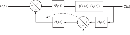
Fig. E3.6(c)
Step 3:The blocks in series as represented by dotted lines in Fig. E3.6(d) can be reduced to a single block as represented in Fig. E3.6(e).

Fig. E3.6(d)
Step 4:The summing point in the feedback as represented by dotted lines in Fig. E3.6(e) can be removed and the resultant block diagram is shown in Fig. E3.6(f).
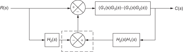
Fig. E3.6(e)
Step 5:In the block diagram as represented by dotted lines in Fig. E3.6(f), the blocks in parallel can be reduced to a single block. In addition, the feedback loop in the block diagram can be reduced. The resultant block diagram is shown in Fig. E3.6(g).

Fig. E3.6(f)
Step 6:The blocks in series as represented in Fig. E3.6(g) can be reduced to a single block to determine the transfer function of the system as shown in Fig. E3.6(a).

Fig. E3.6(g)
Hence, the transfer function of the system is

Example 3.7: For the block diagram of the system shown in Fig. E3.7(a). Determine the transfer function using the block diagram reduction technique when the input R(s) at any instant of time is applied to any one station.

Fig. E3.7(a)
Solution: It is given that the input R(s) at any instant is applied to any one station. Hence, we have two cases for which the transfer function is to be determined.
Case 1: Input R(s) is applied to station I only
The input at station II is made zero and the summing point is removed. The output for the input at station I is C1(s). The block diagram representation with the input R(s) at station-I is shown in Fig. E3.7(b). The transfer function for the block diagram is obtained by applying the block diagram reduction technique to the diagram shown in Fig. E3.7(b).
Step 1:The take-off point that exists before G3(s) block as represented by dotted lines in Fig. E3.7(b) is moved after G3(s) block and the take-off points that exist after G3(s) block are rearranged. The resultant block diagram is shown in Fig. E3.7(c).

Fig. E3.7(b)
Step 2:The feedback loop with the feedback block H2(s) as represented by dotted lines in Fig. E3.7(c) can be reduced. After reduction of the feedback loop, the blocks in series as represented by dotted lines in Fig. E3.7(c) can be multiplied and the resultant block diagram is shown in Fig. E3.7(d).

Fig. E3.7(c)
Step 3:The feedback loop as represented by dotted lines in Fig. E3.7(d) can be reduced. The block diagram after reduction of feedback loop is shown in Fig. E3.7(e).

Fig. E3.7(d)

Step 4:The blocks in series as represented by dotted lines in Fig. E3.7(e) can be reduced to a single block as represented by dotted lines in Fig. E3.7(f).

Fig. E3.7(e)
Step 5:The feedback loop with feedback block H1(s) as indicated by dotted lines in Fig. E3.7(f) can be reduced to determine the closed-loop transfer function of the system represented in Fig. E3.7(a) when the input is applied at station I only.

Fig. E3.7(f)

Therefore,

Case 2: Input R(s) is applied to station II only
The input at station I is made zero and the summing point is removed. In addition, the negative sign in the summing point is attached to the block H1(s). The output for the input at station II is C2(s). The block diagram representation with the input R(s) at station II is shown in Fig. E3.7(g). The transfer function for the block diagram is obtained by applying the block diagram reduction technique to the diagram shown in Fig. E3.7(g).
Step 1:In this step, the blocks in series as indicated by dotted lines in Fig. E3.7(g) can be reduced to a single block. In addition, the summing point that has one of the inputs as H2(s) is shifted before G2(s) and the take-off points that exist after G3(s) are rearranged. The resultant block diagram is shown in Fig. E3.7(h).

Fig. E3.7(g)
Step 2:The two summing points in series as indicated by dotted lines in Fig. E3.7(h) can be interchanged. In addition, the blocks in series can be reduced to a single block. The resultant block diagram is shown in Fig. E3.7(i).

Fig. E3.7(h)
Step 3:The parallel blocks and the feedback loop that exists in the block diagram as indicated by dotted lines in Fig. E3.7(i) can be reduced to a single block as represented in Fig. E3.7(j).

Fig. E3.7(i)
Step 4:The blocks in series as indicated by dotted lines in Fig. E3.7(j) can be reduced to a single block as shown in Fig. E3.7(k).

Fig. E3.7(j)

Step 5:The feedback loop as indicated by dotted lines in Fig. E3.7(k) can be reduced in order to determine the transfer function of the system represented by block diagram as shown in Fig. E3.7(a) when the input R(s) is applied at station II only.
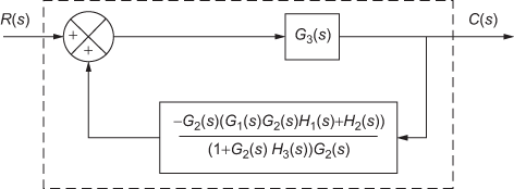
Fig. E3.7(k)


Hence, the transfer function of the multi-input system shown in Fig. E3.7(a) is obtained by considering one input at a time.
Example 3.8: For the block diagram of the system shown in Fig. E3.8(a), determine the transfer function using the block diagram reduction technique.

Fig. E3.8(a)
Solution:
Step 1:The take-off point that exists in the common feedback path as indicated by dotted lines in Fig. E3.8(b) is separated to form two individual feedback paths. The resultant block diagram is shown in Fig. E3.8(c).

Fig. E3.8(b)
Step 2:The blocks in series and the feedback path as indicated by dotted lines in Fig. E3.8(c) can be reduced to form a single block and the resultant block diagram is shown in Fig. E3.8(d).

Fig. E3.8(c)
Step 3:The take-off point that exists between the blocks  and
and ![]() as represented by dotted lines in Fig. E3.8(d) can be shifted after the block
as represented by dotted lines in Fig. E3.8(d) can be shifted after the block ![]() . The resultant block diagram is shown in Fig. E3.8(e).
. The resultant block diagram is shown in Fig. E3.8(e).

Fig. E3.8(d)
Step 4:The blocks in series as indicated by dotted lines in Fig. E3.8(e) can be combined to form a single block and the resultant block diagram is shown in Fig. E3.8(f).

Fig. E3.8(e)
Step 5:The feedback path as represented by dotted lines in Fig. E3.8(f) can be reduced to form a single block and the resultant block diagram is shown in Fig. E3.8(g).

Fig. E3.8(f)
Step 6:The blocks in series as represented by dotted lines in Fig. E3.8(g) can be combined to form a single block and the resultant block diagram is shown in Fig. E3.8(h).

Fig. E3.8(g)
Step 7:The feedback path as indicated by dotted lines in Fig. E3.8(h) can be reduced to form a single block and the resultant block diagram is shown in Fig. E3.8(i).

Fig. E3.8(h)
Step 8:The blocks in parallel as shown in Fig. E3.8(i) can be combined to determine the transfer function of the system.

Fig. E3.8(i)
Hence, the transfer function of the system is given by

Example 3.9: For the block diagram of the system as shown in Fig. E3.9(a), determine the transfer function using the block diagram reduction technique.

Fig. E3.9(a)
Solution:
Step 1:The take-off point that exists after the block ![]() as indicated by dotted lines in Fig. E3.9(b) is shifted before the block
as indicated by dotted lines in Fig. E3.9(b) is shifted before the block ![]() and the resultant block diagram is shown in Fig. E3.9(c).
and the resultant block diagram is shown in Fig. E3.9(c).

Fig. E3.9(b)
Step 2:The blocks in series as represented by dotted lines in Fig. E3.9(c) can be combined to form a single block. The resultant block diagram is shown in Fig. E3.9(d).

Fig. E3.9(c)
Step 3: The feedback path as indicated by dotted lines in Fig. E3.9(d) can be reduced and the resultant block diagram is shown in Fig. E3.9(e).

Fig. E3.9(d)
Step 4:The blocks in series as indicated by dotted lines in Fig. E3.9(e) can be combined to form a single block. The resultant block diagram is shown in Fig. E3.9(f).

Fig. E3.9(e)
Step 5:The feedback path as represented by dotted lines in Fig. E3.9(f) can be reduced and the resultant block diagram is shown in Fig. E3.9(g).
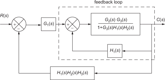
Fig. E3.9(f)
Step 6:The blocks in series as represented by dotted lines in Fig. E3.9(g) can be combined to form a single block. The resultant block diagram is shown in Fig. E3.9(h).

Fig. E3.9(g)
Step 7:The feedback path as indicated by dotted lines in Fig. E3.9(h) can be reduced and the resultant block diagram is shown in Fig. E3.9(i).

Fig. E3.9(h)
Step 8:The block diagram shown in Fig. E3.9(i) can be solved to determine the transfer function of the given system.

Fig. E3.9(i)
Hence, the transfer function of the given system is obtained as

Example 3.10: For the block diagram of the system as shown in Fig. E3.10(a), determine the transfer function using the block diagram reduction technique.

Fig. E3.10(a)
Solution:
Step 1:The summing point that exists after the block ![]() and the take-off point that exists after the block
and the take-off point that exists after the block ![]() as indicated by dotted lines in Fig. E3.10(b) are shifted before the block
as indicated by dotted lines in Fig. E3.10(b) are shifted before the block ![]() and after the block
and after the block ![]() respectively and the resultant block diagram is shown in Fig. E3.10(c).
respectively and the resultant block diagram is shown in Fig. E3.10(c).

Fig. E3.10(b)
Step 2:The blocks in series as indicated by dotted lines in Fig. E3.10(c) are combined to form a single block. The resultant block diagram is shown in Fig. E3.10(d).

Fig. E3.10(c)
Step 3:The summing points that exist between the input signal and the block ![]() as indicated by dotted lines in Fig. E3.10(d) are interchanged and the resultant block diagram is shown in Fig. E3.10(e).
as indicated by dotted lines in Fig. E3.10(d) are interchanged and the resultant block diagram is shown in Fig. E3.10(e).

Fig. E3.10(d)
Step 4:The feedback path as represented by dotted lines in Fig. E3.10(e) can be reduced and the resultant block diagram is shown in Fig. E3.10(f).

Fig. E3.10(e)
Step 5:The blocks in series as indicated by dotted lines in Fig. E3.10(f) are combined to form a single block. The resultant block diagram is shown in Fig. E3.10(g).

Fig. E3.10(f)
Step 6:The feedback path as indicated by dotted lines in Fig. E3.10(g) can be reduced in order to determine the transfer function of the system.
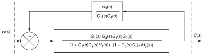
Fig. E3.10(g)
Hence, the transfer function of the given system is obtained as
![]()

Example 3.11: For the block diagram of the system shown in Fig. E3.11(a), determine the transfer function using the block diagram reduction technique.

Fig. E3.11(a)
Solution:
Step 1:The take-off point that exists between the blocks ![]() and
and ![]() as indicated by dotted lines in Fig. E3.11(b) is shifted after the block
as indicated by dotted lines in Fig. E3.11(b) is shifted after the block ![]() . The resultant block diagram is shown in Fig. E3.11(c).
. The resultant block diagram is shown in Fig. E3.11(c).

Fig. E3.11(b)
Step 2:The blocks in series as indicated by dotted lines in Fig. E3.11(c) can be combined to form a single block. The resultant block diagram is shown in Fig. E3.11(d).

Fig. E3.11(c)
Step 3:The blocks in parallel and the feedback loop that exists in the block diagram as indicated by dotted lines in Fig. E3.11(d) can be reduced to form a single block. The resultant block diagram is shown in Fig. E3.11(e).

Fig. E3.11(d)
Step 4:The blocks in series as indicated by dotted lines in Fig. E3.11(e) can be reduced to form a single block. The resultant block diagram is shown in Fig. E3.11(f).

Fig. E3.11(e)
Step 5:The feedback loop that exists in the block diagram shown in Fig. E3.11(f) can be reduced in order to determine the transfer function of the system.

Fig. E3.11(f)
Hence, the transfer function of the system is obtained as

i.e., 
Example 3.12: For the block diagram of the system shown in Fig. E3.12(a), determine the transfer function using the block diagram reduction technique.

Fig. E3.12(a)
Solution:
Step 1:The take-off point that exists between the blocks ![]() and
and ![]() as indicated by dotted lines in Fig. E3.12(b) is shifted after the block
as indicated by dotted lines in Fig. E3.12(b) is shifted after the block ![]() . The resultant block diagram is shown in Fig. E3.12(c).
. The resultant block diagram is shown in Fig. E3.12(c).
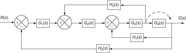
Fig. E3.12(b)
Step 2:The blocks in series as indicated by dotted lines in Fig. E3.12(c) can be combined to form a single block and the resultant block diagram is shown in Fig. E3.12(d).

Fig. E3.12(c)
Step 3:The feedback loop as indicated by dotted lines in Fig. E3.12(d) can be reduced to a single block and the resultant block diagram is shown in Fig. E3.12(e).

Fig. E3.12(d)
Step 4:The blocks in series as indicated by dotted lines in Fig. E3.12(e) can be reduced to a single block and the resultant block diagram is shown in Fig. E3.12(f).

Fig. E3.12(e)
Step 5:The feedback path as indicated by dotted lines in Fig. E3.12(f) can be reduced to form a single block and resultant block diagram is shown in Fig. E3.12(g).

Fig. E3.12(f)
Step 6:The blocks in series as indicated by dotted lines in Fig. E3.12(g) can be reduced to a single block and the resultant block diagram is shown in Fig. E3.12(h).

Fig. E3.12(g)
Step 7:The feedback path as indicated by dotted lines in Fig. E3.12(h) can be reduced to obtain transfer function of the system.

Fig. E3.12(h)
Hence, the transfer function of the system is obtained as

i.e., 
Example 3.13: For the block diagram of the system shown in Fig. E3.13(a), determine the transfer function using the block diagram reduction technique.

Fig. E3.13(a)
Solution:
Step 1:The feedback path as indicated by dotted lines in Fig. E3.13(b) can be reduced and the resultant block diagram is shown in Fig. E3.13(c).

Fig. E3.13(b)
Step 2:The summing point that exists before the block ![]() as indicated by dotted lines in Fig. E3.13(c) is shifted before the
as indicated by dotted lines in Fig. E3.13(c) is shifted before the  and the resultant block diagram is shown in Fig. E3.13(d).

Fig. E3.13(c)
Step 3:The two summing points that exist in the block diagram as indicated by dotted lines in Fig. E3.13(d) are interchanged and the resultant block diagram is shown in Fig. E3.13(e).

Fig. E3.13(d)
Step 4:The blocks in series as indicated by dotted lines in Fig. E3.13(e) can be reduced to form a single block and the resultant block diagram is shown in Fig. E3.13(f).

Fig. E3.13(e)
Step 5:The blocks in parallel and the feedback loop as indicated by dotted lines in Fig. E3.13(f) can be reduced and the resultant block diagram is shown in Fig. E3.13(g).

Fig. E3.13(f)
Step 6:The blocks in series as indicated by dotted lines in Fig. E3.13(g) can be reduced in order to determine the transfer function of the system.

Fig. E3.13(g)
Hence, the transfer function of the system is given by

i.e., 
Example 3.14: For the block diagram of the system shown in Fig. E3.14(a), determine the transfer function using the block diagram reduction technique.

Fig. E3.14(a)
Solution:
Step 1:The take-off point that exists between the blocks ![]() and
and ![]() as indicated by dotted lines in Fig. E3.14(b) is shifted after the block
as indicated by dotted lines in Fig. E3.14(b) is shifted after the block ![]() and the resultant diagram is shown in Fig. E3.14(c).
and the resultant diagram is shown in Fig. E3.14(c).

Fig. E3.14(b)
Step 2:The blocks in series as indicated by dotted lines in Fig. E3.14(c) can be combined to form a single block. The resultant diagram is shown in Fig. E3.14(d).
Fig. E3.14(c)
Step 3:The feedback path as indicated by dotted lines in Fig. E3.14(d) can be reduced and the resultant block diagram is shown in Fig. E3.14(e).

Fig. E3.14(d)
Step 4:The blocks in series as indicated by dotted lines in Fig. E3.14(e) can be combined to form a single block. The resultant block diagram is shown in Fig. E3.14(f).

Fig. E3.14(e)
Step 5:The feedback path as indicated by dotted lines in Fig. E3.14(f) can be reduced in order to determine the transfer function of the system.

Fig. E3.14(f)
Hence, the transfer function of the system is given by

i.e., 
Review Questions
- What do you mean by block diagram representation of a system?
- Explain how an open-loop system can be represented by using a block diagram
- Give the block diagrammatic representation of a generalized closed-loop system.
- What are the advantages of the block diagram representation of a system?
- What are the disadvantages of the block diagram representation of a system?
- Explain with a neat flow chart, how to represent an electrical system with the help of a block diagram.
- What do you mean by block diagram reduction technique?
- What is the necessity for using the block diagram reduction technique?
- What do you mean by block diagram algebra?
- What are the elements present in the block diagram algebra?
- Define: (i) block, (ii) input signal, (iii) forward path, (iv) feedback path, (v) feedback signal and (vi) error signal.
- What do you mean by summing point?
- Define output signal and take-off point.
- What are the lists of rules used for reducing the complex block diagram to a simple one?
- Explain with a neat diagram, the rules for reducing the complex block diagram.
- Explain with a neat flow chart the procedure used for implementing the block diagram reduction technique.
- Represent the electrical circuit shown in Fig. Q3.17 by a block diagram.

Fig. Q3.17
- For the block diagram of the system shown in Fig. Q3.18, determine the transfer function using block diagram reduction technique.

Fig. Q3.18
- For the block diagram of the system shown in Fig. Q3.19, determine the transfer function using the block diagram reduction technique.

Fig. Q3.19
- For the block diagram of the system shown in Fig. Q3.20, determine the transfer function using the block diagram reduction technique.

Fig. Q3.20
- For the block diagram of the system shown in Fig. Q3.21, determine the transfer functions
 and
and  using the block diagram reduction technique.

Fig. Q3.21
- For the block diagram of the system shown in Fig. Q3.22, determine the transfer function using the block diagram reduction technique.

Fig. Q3.22
- For the block diagram of the system shown in Fig. Q3.23, determine the transfer function using the block diagram reduction technique.

Fig. Q3.23
- For the block diagram of the system shown in Fig. Q3.24, determine the transfer function using the block diagram reduction technique.
Fig. Q3.24
- Represent the electrical circuit shown in Fig. Q3.25 by a block diagram.

Fig. Q3.25
- For the system shown in Fig. Q3.26, determine the transfer function using block diagram reduction technique.

Fig. Q3.26
- For the block diagram of the system shown in Fig. Q3.27, determine the transfer function using the block diagram reduction technique.

Fig. Q3.27
- For the block diagram of the system shown in Fig. Q3.28, determine the output using the block diagram reduction technique when (i) each input acts separately on the system and (ii) both the inputs act on the system simultaneously.

Fig. Q3.28
- For the block diagram of the system shown in Fig. Q3.29, determine the output using the block diagram reduction technique when (i) only the input R(s) acts on the system, (ii) only the disturbance input D(s) acts on the system and (iii) both the inputs act on the system simultaneously.
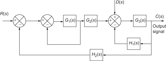
Fig. Q3.29
- For the block diagram of the system shown in Fig. Q3.30, determine the transfer function using the block diagram reduction technique.

Fig. Q3.30
- For the block diagram of the system shown in Fig. Q3.31, determine the transfer function using the block diagram reduction technique.

Fig. Q3.31
- For the block diagram of the system shown in Fig. Q3.32, determine the transfer function using the block diagram reduction technique.

Fig. Q3.32
- For the block diagram of the system shown in Fig. Q3.33, determine the transfer function using the block diagram reduction technique.

Fig. Q3.33