8

FREQUENCY RESPONSE ANALYSIS

8.1 Introduction

After obtaining the mathematical model of the system, its performance is analysed based on the time response or frequency response. Time response of the system is defined as the response of the system when standard test signals such as impulse, step and so on are applied to it. Frequency response of the system is defined as the response of the system when standard sinusoidal signals are applied to it with constant amplitude over a range of frequencies. The frequency response indicates the steady-state response of a system to a sinusoidal input. The characteristics and performance of the industrial control system are analysed by using the frequency response techniques. Frequency response analysis is used in ­numerous systems and components such as audio and video amplifiers, speakers, sound cards and servomotors. The different techniques available for frequency response analysis lend themselves to a simplest procedure for experimental testing and analysis. In addition, the stability and relative stability of the system for the sinusoidal input can be analysed by using different frequency plots.

This chapter introduces the frequency response of the system and explains the procedure for construction of Bode plot to determine frequency domain specifications such as gain crossover frequency, phase crossover frequency, gain margin and phase margin.

8.1.1 Advantages of Frequency Response Analysis

The time response of the system can be obtained only if the transfer function of the system is known earlier, which is always not possible. But it is possible to obtain frequency response of the system even though the transfer function of the system is not known. The reasons for determining the frequency response of the system are:

1. Analytically, it is more difficult to determine the time response of the system for higher order systems.
2. As there exists numerous ways of designing a control system to meet the time domain performance specifications, it becomes difficult for the designer to choose a suitable design for a particular system.
3. The transfer function of a higher order system can be identified by computing the frequency response of the system over a wide range of frequencies .
4. The time-domain specifications of a system can be met by using the frequency domain specifications as a correlation exists between the frequency response and time response of a system.
5. The stability of a non-linear system can be analysed by the frequency response ­analysis.
6. The transfer function of a higher order system can be obtained using frequency response analysis which makes use of physical data when it is difficult to obtain using differential equations.
7. The frequency response analysis can be applied to the system that has no rational transfer function (i.e., a system with transportation lag).
8. The frequency response analysis can be applied to the system even when the input is not deterministic.
9. The frequency response analysis is very convenient in measuring the system ­sensitivity to noise and parameter variations.
10. In frequency response analysis, stability and relative stability of a system can be analysed without evaluating the roots of the characteristic equation of the system.
11. The frequency response analysis is simple and accurate.

8.1.2 Disadvantages of Frequency Response Analysis

The disadvantages of frequency response analysis are:

1. Frequency response analysis is not recommended for the system with very large time constants.
2. It is not useful for non-interruptible systems.
3. It can generally be applied only to linear systems. When this approach is applied to a non-linear system, the result obtained is not exact.
4. It is considered as outdated when compared with the methods developed for digital computer and modelling.

The comparison between the time response analysis and frequency response analysis is listed in Table 8.1.

Table 8.1 ∣ Comparison between the time response analysis and frequency response analysis

8.2 Importance of Sinusoidal Waves for Frequency Response Analysis

In frequency response analysis, the signal used as an input to the system is a sinusoidal wave because of the following reasons:

1. Fourier theory (infinite sum of sine wave and cosine wave).
2. Any input signal applied to the circuit can be represented as a combination of sine and cosine waves of different frequencies and amplitudes.

Consider a ramp signal as shown in Fig. 8.1(a) and constant sine and cosine waves of varying amplitude as shown in Fig. 8.1(b).

Fig. 8.1 ∣ (a) Ramp signal, (b) Fourier components and (c) original and sum of fourier components

If the sine wave and cosine wave as shown in Fig. 8.1(b) are added, the resultant will be a ramp signal indicated using a dotted line along with the original ramp signal shown as a continuous line depicted in Fig. 8.1(c). Since any signal can be represented by varying the frequency and amplitude of the sine and cosine waves, the sinusoidal wave is chosen for frequency domain analysis.

8.3 Basics of Frequency Response Analysis

The steady-state output of the stable linear system is also a sine wave of same frequency when a sinusoidal input is applied to the system. The output and input of the system generally differs in both magnitude and phase. Generally, the frequency response of the system can be obtained by replacing the variable s in the transfer function with as given by

(8.1)

where is the magnitude or gain i.e., the sinusoidal amplitude ratio of output to input. In addition, is the angle by which the output leads the input. The parameters and are functions of the angular frequency . The Laplace variable s is a complex number that is represented as . If a linear time-invariant system is subjected to a pure sinusoidal input, , the output response of the system contains both the transient part and the steady-state part. But at , the transient part dies out because the roots have negative parts for a stable system and only the steady-state part of the output response exists. Therefore, as the frequency response of the system deals with steady-state analysis of the system, it is enough to substitute instead of .

Fig. E8.1

Solution: The transfer function of the low-pass RC network is

Substituting the values of and , we obtain

The Laplace transform of the input,

Hence, the output of the system,

Using partial fractions, we obtain

Taking inverse Laplace transform, we obtain

where is the transient part of the output and is the steady-state part of the output.

8.4 Frequency Response Analysis of Open-Loop and Closed-Loop Systems

The frequency response analysis of both open-loop and closed-loop systems is discussed below.

8.4.1 Open-Loop System

Fig. 8.2 ∣ A simple open-loop system

Consider an open-loop linear time-invariant system as shown in Fig. 8.2. The input signal i.e., sinusoidal with amplitude and frequency is given by

The steady-state output of the system will also be a sinusoidal function with the same frequency but possibly with a different amplitude and phase, i.e.,

where is the amplitude of the output sinusoidal wave and is the phase shift in degrees or radians.

Let the transfer function of a linear single-input single-output (SISO) system be . Then, the relation between the Laplace transforms of the input and the output is

For sinusoidal steady-state analysis i.e., frequency response analysis, s is replaced with Then, the above equation becomes

(8.2)

Here, can be written in terms of magnitude and phase angle as

(8.3)

Similarly, Eqn. (8.2) can be re-written as

(8.4)

Hence, comparing Eqs. (8.3) and (8.4), we obtain

(8.5)

and the phase angle is

(8.6)

From the transfer function of a linear time-invariant system with sinusoidal input, the magnitude and phase angle of the output can be obtained using Eqs. (8.5) and (8.6) ­respectively.

8.4.2 Closed-Loop System

Fig. 8.3 ∣ A simple closed-loop system

The closed-loop system is shown in Fig. 8.3.

The transfer function

For the frequency response analysis, substituting , we get

The transfer function can be expressed in terms of its magnitude and phase as

Therefore, the magnitude of is

(8.7)

The phase angle of is

(8.8)

Thus, by knowing the transfer function of a linear time-invariant system and the feedback transfer function the magnitude and phase angle of the output for the closed-loop system can be obtained using Eqs. (8.7) and (8.8) respectively, provided the input to the system is sinusoidal.

8.4.3 Closed-Loop System with Poles and Zeros

Consider a negative feedback closed-loop system as shown in Fig. 8.3 with the closed-loop transfer function as

(8.9)

where is the Laplace transform of the output and is the Laplace transform of the input.

For a closed-loop stable system,

(8.10)

where, and

where and are positive and distinct integers with .

Consider the input applied to the system as

Taking Laplace transform, we obtain

Hence, the Laplace transform of the output using Eqn. (8.9) is

Substituting Eqn. (8.10) in the above equation, we obtain

Using partial fractions for the above equation, we obtain

(8.11)

Here, , where

In addition,

As the constant K₁ is a complex number, it is convenient to represent it in polar form as

where

Since we have assumed all the values of the steady-state response is

Thus, if a sinusoidal input is applied to a system that has negative real value of poles, the steady-state response is a scaled, phase-shifted version of the input. The scaling factor is and the phase shift is the phase of .

8.5 Frequency Response Representation

The frequency response analysis of a system is used to determine the system gain and phase angle of the system at different frequencies. Hence, the system gain and phase angle can be represented either in a tabular form or graphical form.

Tabular form: It is useful in representing the system gain and phase angle of a system at different frequencies only if the data set is relatively small. It is also useful in experimental measurement.

Graphical form: It provides a convenient way to view the frequency response data. There are many ways of representing the frequency response in the graphical form.

8.5.1 Determination of Frequency Response

The frequency response analysis of a system can be determined using (i) experimental determination and (ii) mathematical determination.

(i) Experimental determination of frequency response

This method is used only when the system transfer function is not known. This method is used for a plant testing and verification of the plant model. Determining the frequency response of a the small system experimentally in a laboratory environment is not very difficult. A typical set-up for the experimental determination of the frequency response is shown in Fig. 8.4.

Fig. 8.4 ∣ Experimental set-up for frequency response

The requirement for determining frequency response varies for different systems. The ­general requirements for determining the frequency response of systems are power supply, signal generator and a chart recorder or dual trace oscilloscope. The experimental set-up varies depending on the test systems.

The steps to be followed for determining the frequency response are:

1. Test frequency range and input signal amplitude are established.
2. Sinusoidal signal with low frequency is applied and sufficient time is allowed for settling of transients present in the system.
3. After a stable output is reached, using the input and output waveforms, the system gain and phase angle are determined.
4. The same procedure can be applied for the input signal with different frequencies and the frequency response analysis of the system can be determined.

Thus, the frequency response of the system whose transfer function is not known can be determined.

Mathematical evaluation of frequency response

This method is applicable to the system whose transfer function is known. In this method, by substituting , the transfer function is considered to be a function of frequency and it is treated as a complex variable. The system gain and phase angle at a particular frequency is same as the magnitude and phase angle of the complex number.

The mathematical procedure for determining the frequency response of simple and complex transfer functions are given below:

Simple transfer function

1. Choose the frequency for which the frequency response has to be determined.
2. Substitute in the given transfer function.
3. Convert the resultant complex number into a polar form.
4. Substitute the chosen frequency in the above equation and determine the magnitude and angle of the complex number.
5. Then, the system gain and phase angle at that particular frequency are determined.
6. Repeat the above steps for different frequencies and the corresponding system gain and the phase angle can be tabulated.

Complex transfer function

A complex transfer function can be separated in two simple transfer functions and each simple transfer function can be converted into the polar form. The complex number in polar form allows easier manipulation of magnitude and angle. The procedure is as follows:

1. Convert the complex transfer function into a product of simple transfer functions.
2. For each simple transfer function, follow the steps that have been discussed earlier to determine the individual magnitude and angle of the simple transfer functions.
3. Then, the overall gain and phase angle of the complex transfer function at a particular frequency can be obtained by multiplying the individual gain and adding the phase angles, respectively.
4. The above steps can be repeated for different frequencies and the system gain and phase angle can be determined.

Solution:

Gain of the complex system = product of gains of simple systems

Phase angle of the complex system = addition of phase angles of simple systems

The given complex system can be divided into four simple functions as

Simple system 1:

Substituting , we obtain

Therefore, gain of the system M₁ = 5 and phase angle of the system = 0°.

Simple system 2

Substituting , we obtain

Therefore, gain of the system M₂ = and phase angle of the system

Simple system 3

Substituting , we obtain

Therefore, gain of the system, M₃ =

and phase angle of the system

Simple system 4

Therefore,

Therefore, gain of the system

and phase angle of the system

The gain and the phase angle of various simple systems at different frequencies between 0.1 and 10 rad/sec are calculated and tabulated as given in Tables E8.3(a) and (b) respectively.

Table E8.3(a) ∣ Gain of the simple systems at different frequencies

Table E8.3(b) ∣ Phase angle of the system at different frequencies

Therefore, the overall gain and phase angle of the complex system is determined using the following expressions and are tabulated in Table E8.3(c).

Gain of the system,

Phase angle of the system, .

Table E8.3(c) ∣ Gain and phase angle of the complex system at different frequencies

8.6 Frequency Domain Specifications

Frequency domain specifications of a system are necessary to determine the quality of the system and to design the linear control systems using frequency domain analysis.

Consider a simple closed-loop system as shown in Fig. 8.3. Its transfer function is

The magnitude or gain of the above transfer function as a function of frequency is given by

The phase angle of the transfer function as a function of frequency is given by

The typical gain–phase characteristics of a feedback control system are shown in Figs. 8.5(a) and (b).

Fig. 8.5 ∣ Gain–phase characteristics

The different frequency domain specifications that are required for designing a control system and determining its performance are:

(i) Resonant peak M_r

The maximum value of gain as the frequency of the system is varied over a range is known as resonant peak . The relative stability of the system can be determined based on this value. There exists a direct relationship between the maximum overshoot in the time-domain analysis of the system and the resonant peak in the frequency domain analysis (i.e., a large value of indicates that the maximum overshoot of the system is also large). The resonant peak lies between 1.1 and 1.5.

(ii) Resonant frequency

The frequency of the system at which the resonant peak occurs is known as resonant frequency . The frequency of oscillations in the time domain is related to the resonant frequency . When resonant frequency is high, the time response or transient response of the system is fast.

(iii) Cut-off frequency

The frequency at which the gain of the system is 3 dB or 0.707 times the gain of the system at zero frequency is known as cut-off frequency .

(iv) Bandwidth

The range of frequencies that lie between zero and is known as bandwidth. It is also defined as the range of frequencies over which the magnitude response of the system is flat.

The value of bandwidth indicates the ability of the system to reproduce the input signal and it is a measure of the noise rejection characteristics. In time-domain analysis of the system for a given damping factor, bandwidth in the frequency domain indicates the rise time in the time domain. If the bandwidth of the system in the frequency domain is large, then the rise time of the system in time domain is small and the system will be faster.

(v) Cut-off rate

The slope of the magnitude curve obtained near the cut-off frequency is called cut-off rate. The cut-off rate indicates the ability of the system to distinguish the signal from noise.

(vi) Gain crossover frequency

The frequency at which the gain of the system is unity is called the gain crossover frequency .

If the gain of the system is expressed in dB, then the gain crossover frequency is defined as the frequency at which the gain of the system is 0 dB (since 20 log 1 = 0 dB).

(vii) Phase crossover frequency

The frequency at which the phase angle of the system is −180° is called phase crossover frequency.

(viii) Gain margin g_m

In root locus technique, there exists a relationship between the gain and stability of the system. Similarly, in frequency response method, there exists a value of K, beyond which the system becomes unstable. Hence, the gain margin is defined as the factor by which the gain of the system can be increased before the system becomes unstable. Mathematically, it is defined as the reciprocal of the gain of the system at the phase crossover frequency .

The stability of the system is directly proportional to the gain margin of the system. In addition, the high gain margin results in an unacceptable response and the result becomes sluggish in nature.

(ix) Phase margin p_m

In frequency response analysis, gain margin alone is not sufficient to comment on the relative stability of the system. The other factor that affects the relative stability of the system is phase margin . It is defined as the additional phase lag that makes the system marginally stable. In addition, it can be defined as the addition of phase angle of the system at gain crossover frequency and 180°.

As a thumb rule, for a good overall stability of the system, the gain margin of the system should be around 12 dB and the phase margin should be between 45° and 60°.

8.7 Frequency and Time Domain Interrelations

The interrelation between the time-domain analysis and frequency domain analysis of the system is explicit for the first order. In this section, the interrelation existing between the time domain and frequency domain for a second-order system is discussed. In addition, the ­frequency domain specifications for the second-order system are derived using the ­frequency response analysis.

Consider a second-order system as shown in Fig. 8.6 with the feed-forward transfer function as and with a unity feedback.

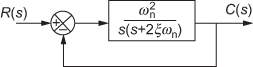
Fig. 8.6 ∣ A simple second order system

Hence, the transfer function of the second-order system is given by

(8.12)

where is the damping ratio of the system and is the undamped natural frequency of the system.

In addition,

The transfer function of the system in frequency domain is obtained by substituting in Eqn. (8.12) given by

(8.13)

Substituting in Eqn. (8.13), we obtain (8.14)

where is the normalized driving signal frequency.

Therefore, (8.15)

Using Eqs. (8.14) and (8.15), we obtain (8.16)

and (8.17)

The steady-state output of the system when the system is excited by the sinusoidal input with unit magnitude and variable frequency (i.e., ) is given by

Using Table 8.1, the magnitude and phase angle plots with respect to the normalized frequency u are shown in Figs. 8.7(a) and 8.7(b) respectively.

Table 8.2 ∣ Magnitude and phase values

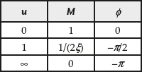
Fig. 8.7 ∣ (a) Magnitude and (b) phase angle plots of second-order system

8.7.1 Frequency Domain Specifications

(i) Resonant frequency ω_r

At resonant frequency , the first-order derivative of the magnitude of frequency domain analysis is zero.

i.e.,

Since the magnitude in Eqn. (8.16) depends on the normalized frequency , the above equation can be written as

where is the normalized resonant frequency.

Therefore,

Simplifying, we obtain

We know that, .

Therefore, the resonant frequency is given by (8.18)

(ii) Resonant peak M_r

The magnitude at resonant frequency , is known as the resonant peak .

i.e.,

Since the magnitude depends on the normalized frequency, the above equation can be written as

Substituting the in Eqs. (8.16) and (8.17), we obtain

(8.19)

(8.20)

But we know that in time domain analysis of a second-order system,

Peak overshoot, (8.21)

Damped natural frequency, (8.22)

From Eqs. (8.19) to (8.22), it is clear that there exists a relationship between the time-domain analysis and frequency domain analysis of a system.

Interesting facts about the interrelation between time-domain analysis and frequency domain analysis of a second-order system are given below.

1. For relative stability of the system, the values of peak overshoot and resonant peak of the system are:

   Peak overshoot

   Resonant peak

   If is greater than 1.5 and the system is subjected to noise signals, then the system may face serious problems.

2. Variation of with respect to the variation in
   1. As increases, the value of peak overshoot, gets decreased and it becomes zero or gets vanished at .

      The resonant peak will also get vanished as the damping ratio ­increases. But the value of at which the resonant peak vanishes is derived as

      

      Therefore,

      Hence, at , the resonant peak and peak overshoot vanished.

      This concept is shown in Figs. 8.8(a) and (b).

      

      Fig. 8.8 ∣ M_p and M_r for different values of

   2. When :

      The gets the maximum value i.e., . In addition, ­approaches infinity as decreases to zero. This concept is shown in Figs. 8.9(a) and (b) respectively.

      

      Fig. 8.9 ∣ M_p and M_r for x = 0

3. Choosing the value of damping ratio :

   The damping ratio should be chosen between 0.4 and 0.707 (i.e., 0.4 < < 0.707) to have a tolerable and . If the chosen is less than 0.4, both have larger values that are not desirable for the system.

4. Variations of and with respect to :

   When the value of is chosen between 0.4 and 0.707, the value of and are ­comparable to each other.

   When , both the values of and approach .

   When is small, then the values of and are:

   1. will be large and hence the rise time is small.
   2. will be large and the response of the system will be faster.

   Here, the value of indicates the speed of the response. The above concept is shown in Figs. 8.10(a) and (b).

   

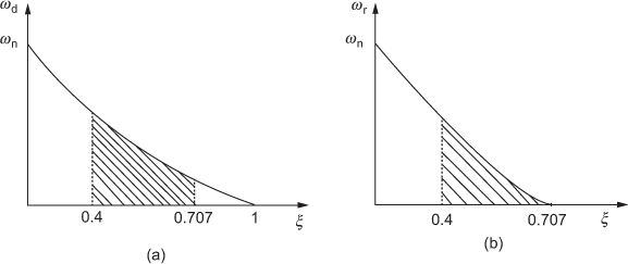
   Fig. 8.10 ∣ ω_d and ω_r for different values of ξ

(iii) Bandwidth

The range of frequencies between zero and cut-off frequency , is known as bandwidth and the cut-off frequency is defined as the frequency at which the magnitude of the system is 3 dB down the magnitude of the system at zero frequency. Hence, bandwidth is nothing but the cut-off frequency .

Assuming the magnitude of the system at zero frequency as 1, the cut-off frequency is derived as

= =

But from Eqn. (8.16), it is clear that the magnitude depends on the normalized frequency. Hence, the above equation can be written as

=

Comparing the above equation with the quadratic equation , we obtain

Hence, solving this quadratic equation, we obtain

Considering only the positive values, we obtain

Therefore, (8.23)

We know that,

Therefore, the cut-off frequency is given by (8.24)

The expression for bandwidth is also same as that of the cut-off frequency. From Eqn. (8.23), the normalized bandwidth is equal to 1. The graphical idea about the bandwidth with respect to the damping ratio is shown in Fig. 8.11.

Fig. 8.11 ∣ Magnitude versus frequency

The graphical idea between the normalized bandwidth and the damping ratio is shown in Fig. 8.12.

Fig. 8.12 ∣ ξ vs normalized bandwidth

Solution: Given and .

Hence, the closed-loop transfer function of the system,

The characteristic equation of the given system is

Comparing the above equation with the standard second-order characteristic , we obtain

, i.e., rad/sec and , i.e.,

Hence,

Resonant peak,

Resonant frequency, rad/sec

Solution: The closed-loop transfer function of any system is given by

and the characteristic equation of the system is given by

The closed-loop poles of a system are obtained by equating the characteristic equation to zero. Hence, the characteristic equation of the given system using the given closed-loop poles is obtained as

i.e.,

Comparing the above equation with the standard second-order characteristic equation, we obtain . Therefore, rad/sec

Therefore,

Using the damping ratio and natural frequency, the frequency domain specifications can be determined as given below:

1. Bandwidth (BW) =

   = 4.350 rad/sec

2. Normalized peak driving signal frequency () is

   = = 0.3846

3. Resonant peak,

   Therefore, = = 1.083

Solution: Given = 4 rad/sec and = 1.6 rad/sec

We know that

Therefore,

Upon solving, we obtain

1. Peak overshoot when subjected to step input =
2. Resonance peak,

Solution: Given and

We know that

i.e.,

i.e.,

Upon solving, we obtain

i.e., or 0.933

Therefore, or 0.966

The system with the damping ratio greater than 0.707 does not exhibit any peak in the ­frequency response of the system. Hence, the damping ratio of the given system is .

We know that,

Substituting the known values, we obtain

Upon solving, we obtain rad/sec

The standard second-order transfer function of the system is

Substituting the known values, we obtain

=

Here, rad

Therefore, rad

Also, rad/sec

Rise time, = 0.2957 sec

Peak time, = 0.5045 sec

Settling time for a system can be determined for 2% error tolerance and 5% error tolerance.

Hence, sec for 2% tolerance

sec for 5% tolerance

Period of oscillation, sec

Number of oscillations before the response of the system gets settled is given by

Peak overshoot of the system is = 0.4309

Determine the frequency response parameters of the system (i) peak resonance , (ii) resonant frequency and (iii) cut-off frequency of the system .

Solution:

From the given Table, the maximum value of the time response and the peak time of the system are 1.12 and 0.2 s, respectively.

Hence, there exists a peak overshoot of 0.12 at 0.2 sec.

Therefore,

Solving the above equation, we obtain

i.e.,

Therefore, rad/sec

rad/sec

Fig. E8.9

Solution: Given and

Hence, the closed-loop transfer function of the system is

Comparing the above equation with the standard second-order transfer function, we obtain

i.e., (1)

i.e., (2)

Using the values of resonant peak and the resonant frequency, the values of K and a can be determined.

1. 

   i.e.,

   Upon solving, we obtain

2. 

   i.e.,

   Upon solving, we obtain rad/sec

   Substituting the values of in Eqs. (1) and (2), we obtain

   

3. Settling time, sec
4. Bandwidth,

Solution: Given and rad/sec

rad/sec

Solution:

Given

i.e.,

Therefore,

i.e.,

or

i.e.,

Therefore, damping ratio,

Hence, resonant peak,

Solution: Comparing denominator of the transfer function with , we obtain

i.e., and i.e.,

and rad/sec

8.8 Effect of Addition of a Pole to the Open-Loop Transfer ­Function of the System

Consider a system with the open-loop transfer function . When a pole at is added to such a system, the open-loop transfer function of the system becomes . When a sinusoidal input is applied to such a system, the system becomes less stable compared to the stability of the previous system. In addition, the specifications of the frequency domain and time domain vary depending on the time constant .

For larger values of , we obtain

1. Larger rise time that in turn decreases the bandwidth of the system.
2. Larger value of resonant peak that corresponds to a larger value of maximum overshoot in the time response of the system.

8.9 Effect of Addition of a Zero to the Open-Loop Transfer ­Function of the System

Consider a system with the open-loop transfer function . When a zero at is added, the open-loop transfer function of the system becomes . When a sinusoidal input is applied to the system, the following changes occur in the ­frequency domain specifications.

1. Bandwidth of the system gets increased.
2. Increase in time constant for higher values of T_z.
3. Settling time of the system gets increased.

8.10 Graphical Representation of Frequency Response

Determining the frequency response of a system, i.e., the magnitude and phase angle of a system for different frequencies from 0 to by using tabulation method becomes more complicated when more number of poles and zeros exist in the system. An alternative method that eliminates the difficulty of the tabulation method is the graphical representation of frequency response.

There are different graphical methods by which the frequency response can be represented. They are

1. Bode plot (asymptotic plots)
2. Polar plot
3. Nyquist plot
4. Constant M and N circles
5. Nichols chart

The Bode plot of representing frequency response of a system is discussed in this chapter and the other plots will be discussed in the subsequent chapters.

8.11 Introduction to Bode Plot

Bode plot introduced by H.W. Bode was first used in the study of feedback amplifiers. It is one of the popular graphical methods used for determining the stability of the system when the system is subjected to sinusoidal input. The stability of the closed-loop system is determined based on the frequency response of the loop transfer function of the system, i.e., . The gain or magnitude and phase angle of the system can be easily represented as a function of frequency using Bode plot. It is also a very useful graphical tool in analysing and designing of linear control systems.

The Bode plot consists of two plots:

1. Magnitude plot: To plot the logarithmic magnitude or gain of the loop transfer function in dB versus frequency i.e., .
2. Phase plot: To plot the phase angle of the loop transfer function versus frequency i.e., .

In Bode plot, both the magnitude and phase plots are plotted against the frequency in the logarithmic scale. In addition, the magnitude of the system is plotted in dBs (decibels). Hence, the Bode plot is also called logarithmic plot. Since the magnitude and phase plots of a system are sketched based on the asymptotic properties instead of detailed plotting, the Bode plot is also called asymptotic plots.

8.11.1 Reasons for Using Logarithmic Scale

The reasons for plotting the magnitude and phase angle plots of the Bode plot in a logarithmic scale are:

1. In higher order systems, magnitudes of the individual subsystem have to be multiplied to get the magnitude of the higher order system that is a tedious process. But if we use the logarithmic scale, the multiplication part can be replaced by the addition that makes the process of determining the magnitude of the higher order system easier.
2. In addition, the variation of frequency in a large scale is easier if we use a logarithmic scale rather than the ordinary scale.

It is noted that in Bode plot, the magnitude of the loop transfer function is taken in terms of decibels (complex logarithm) rather than the simple logarithm. The magnitude used to plot the magnitude plot in Bode plot is determined using

dB

Table 8.3 shows the importance of logarithmic scale rather than the ordinary scale. Any real value existing between and 100 can be plotted between −40 to 40 dB.

Table 8.3 ∣ The dB values for the original magnitude

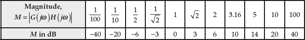
Thus a wide range of magnitude can be plotted easily using logarithmic magnitude scale.

8.11.2 Advantages of Bode Plot

The advantages of using Bode plot in plotting the frequency response of a system are:

1. Expansion of frequency range of a system is simple.
2. Experimental determination of transfer function of a system is simpler if the frequency response of the system is shown using Bode plot.
3. Usage of asymptotic straight lines for approximating the frequency response of the system.
4. Bode plot can be plotted for complicated systems.
5. Relative stability of the closed-loop system can be analysed by plotting the frequency response of the loop transfer function of the system using Bode plot.
6. Frequency domain specifications such as gain crossover frequency, phase crossover frequency, gain margin and phase margin can easily be determined.
7. The variation of frequency domain specifications can easily be viewed when a controller is added to the existing system.
8. The system gain K can be designed based on the required gain and phase margins.
9. Polar plot and Nyquist plot can be constructed based on the data obtained from Bode plot.

8.11.3 Disadvantages of Bode Plot

The disadvantages of using Bode plot in plotting the frequency response of a system are:

1. Using Bode plot, it is possible only to determine the absolute and relative stability of the minimum phase system.
2. Corrections are to be made in the obtained plot to meet the desired frequency plot.

8.12 Determination of Frequency Domain Specifications from Bode Plot

The different frequency domain specifications that can easily be determined using Bode plot are gain margin, phase margin, gain crossover frequency and phase crossover frequency. The plot shown in Fig. 8.13 indicates the determination of the above said frequency domain specifications.

Fig. 8.13 ∣ Frequency domain specifications

From the above plot, the formula for determining the frequency domain specifications can be obtained as follows:

Gain crossover frequency, = frequency at which = 0.

Phase crossover frequency, = frequency at which = −180°.

Gain margin, = 0 dB −.

Phase margin, = − (−180°) = 180°+ phase angle at .

8.13 Stability of the System

The stability of the system is easier to determine using Bode plot once the frequency domain specifications are obtained. The stability of the system can be analysed on the basis of ­crossover frequencies ( and ) or gain and phase margins.

8.13.1 Based on Crossover Frequencies

The system can either be a stable system, marginally stable system or unstable system. The stability of the system based on the relation between crossover frequencies is given in Table 8.4.

Table 8.4 ∣ Stability of the system based on crossover frequencies

8.13.2 Based on Gain Margin and Phase Margin

The stability of the system based on the gain margin and phase margin is given in Table 8.5.

Table 8.5 ∣ Stability of the system based on g_m and p_m

8.14 Construction of Bode Plot

The construction of Bode plot can be illustrated by considering the generalized form of loop transfer function is given by:

where are real constants,

Z is the number of zeros at the origin,

N is the number of poles at the origin or the TYPE of the system,

M is the number of simple poles existing in the system,

U is the number of simple zeros existing in the system,

V is the number of complex poles existing in the system

Q is the number of complex zeros existing in the system and

T is the time delay in seconds.

Substituting and simplifying, we obtain

Rearranging the above equation, we obtain

(8.25)

where , and

The magnitude of Eqn. (8.25) in dB is given by

The phase angle of Eqn. (8.25) is given by

where magnitude of the term is 1 and phase angle of the term is .

It is noted that phase angle of the term = 0^°.

From Eqn. (8.25), it is clear that the open-loop transfer function may ­contain the combination of any of the following five factors:

1. Constant K.
2. Zeros at the origin and poles at the origin .
3. Simple zero and simple pole .
4. Complex zero and complex pole .
5. Transportation lag .

   Hence, it is necessary to have a complete study (magnitude and phase plots) of these ­factors that can be utilized in constructing the plot (magnitude and phase plots) of a ­composite loop transfer function . The composite plot for the loop transfer function is constructed by adding the plots of individual factors present in the ­function. Thus Bode plot is an approximate asymptotic plot of individual factors.

Factor 1: Constant K

The magnitude and phase angle of the constant K which are to be plotted in a semi log graph sheet are:

Magnitude in dB = .

Phase angle = 0°.

The magnitude and phase plots corresponding to the values obtained using the above equation are shown in Figs. 8.14(a) and (b) respectively.

Fig. 8.14 ∣ Bode plot for factor K

Note:

1. The constant K can have a value that is either greater than 1 or less than 1. The magnitude corresponding to the gain that is greater than 1 is positive and gain that is less than 1 is negative.
2. If the gain K is varied, the corresponding changes occur only in the magnitude plot (i.e., either the plot raises or lowers). If the gain value is increased by a factor 10, then the corresponding magnitude plot gets raised by 20 dB. Similarly, if the gain value is decreased by a factor 10, then the corresponding magnitude plot gets decreased by 20 dB. The proof of this concept is given below.

   

   Similarly,

3. In addition, if the magnitude of a constant K is expressed in dB, the magnitude of ­reciprocal of the particular constant K in dB will have the same value but the sign ­differs.

   i.e.,

Factor 2: Zeros at the origin or poles at the origin

In Bode plots, the frequency ratios are expressed in terms of octaves or decades. When the frequency band is from to , it is called decade.

The details for plotting the magnitude and phase plots when only one pole or zero exists at the origin are given in Table 8.6.

Table 8.6 ∣ Magnitude and phase plots for and

 

The magnitude in dB will be equal to zero at the frequency value of .

If multiple poles or zeros exist at the origin, the corresponding changes in the magnitude and phase plots are given in Table 8.7. Let the number of zeros at the origin existing in the system be Z and the number of poles at the origin be N.

Table 8.7 ∣ Magnitude and phase plots for and

Factor 3: Simple pole or simple zero

The details for plotting the magnitude and phase plots when only one simple pole or simple zero exists are given in Table 8.8.

Table 8.8 ∣ Magnitude and phase angle for simple pole and simple zero

It is known that the magnitude of a number is same as the magnitude of the reciprocal of a number with the opposite sign. Hence, in this case the step-by-step procedure for plotting the magnitude and phase plots for a simple pole are discussed.

For simple pole

Magnitude plot

1. The magnitude of the simple pole in dB is .
2. Consider two cases:

   Case 1: For low frequencies

   Magnitude =

   Slope =

   Case 2: For high frequencies

   Magnitude =

   The slope of the line is determined as follows:

   At , magnitude = 0 dB

   At , magnitude = −20 dB

   Hence, the slope of the line is

3. Hence, the magnitude plot of the simple pole can be approximated using the two straight-line asymptotes
   1. Straight line at 0 dB .
   2. Straight line with the slope of

   The approximate magnitude plot of the simple pole is shown in Fig. 8.15(a).

   

   Fig. 8.15 (a) ∣ Approximate magnitude plot for

Corner frequency

The frequency at which two asymptotes meet is called corner frequency or break frequency. In this case, the corner frequency is at . The corner frequency divides the frequency response curve of the system as low-frequency region and high-frequency region.

Error in the magnitude plot

The magnitude plot obtained using the above three steps is an approximated magnitude curve. The actual magnitude curve can be obtained by substituting different values of in magnitude equation of simple pole as given in Table 8.9.

Table 8.9 ∣ Actual magnitude curve

Hence, an error exists in the magnitude plot. The error in the magnitude plot is maximum at the corner frequency and the value of the error is obtained by

Error =

The values of error at different frequencies are given in Table 8.10.

Table 8.10 ∣ Error versus Frequency

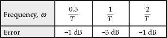
The magnitude plot with the approximate curve and actual curve is shown in Fig. 8.15(b).

Fig. 8.15 (b) ∣ Magnitude plot for (1 + jωT)⁻¹

Phase plot

1. The phase angle for a simple pole is .
2. The phase plot for a simple pole is obtained by substituting different values of .

   At , phase angle = 0°

   At , phase angle = −45°

   At , phase angle = −90°

   Hence, the phase plot of a simple pole is shown in Fig. 8.15(c).

   

   Fig. 8.15 (c) ∣ Approximate phase plot for (1 + jωT)⁻¹

The phase plot of a simple pole is skew symmetric about the inflection point at phase angle = −45°.

Some errors exist in the phase plot when the actual value is approximated and the approximate phase angle value and actual phase angle at different frequencies are given in Table 8.11.

Table 8.11 ∣ Exact and approximate phase values for simple zero

The phase plot with the approximate curve and actual curve are shown in Fig. 8.15(d).

Fig. 8.15 (d) ∣ Phase plot for a simple pole

For simple zero

The reciprocal of a simple pole is a simple zero. Hence, the magnitude and phase plots of a simple zero are just the mirror image of the plots of simple pole. The magnitude and phase plots of a simple zero with the actual curve and approximated curve are shown in Figs. 8.15(e) and (f) respectively.

Fig. 8.15 ∣ Bode plot for simple zero (1 + jωT)⁻¹

If the number of simple poles and simple zeros of same value existing on the system is , then the magnitude and phase plots are obtained as

1. Corner frequency is the same i.e., .
2. Low-frequency asymptote is a horizontal straight line at .
3. High-frequency asymptote is a straight line with the slope of
4. The phase angle in the phase plot of the system is times the phase angle of the simple pole or simple zero at each frequency.
5. Error in each plot is times the error of simple pole or simple zero.

Factor 4: Complex zero and complex pole

The details for plotting the magnitude and phase plots of complex pole and complex zero is given in Table 8.12.

Table 8.12 ∣ Magnitude and phase angle for complex zero and complex pole

In Table 8.12, is the damping ratio and .

It is known that the magnitude of a number is same as the magnitude of the reciprocal of that number with opposite sign. The magnitude and phase plots of the quadratic factor depend on the corner frequency and the damping factor. Hence, in this case, the step-by-step procedure for plotting the magnitude and phase plots for simple poles has been discussed.

8.14.1 Effect of Damping Ratio

When the damping ratio is greater than 1, i.e., , the quadratic factor can be written as the product of two first-order factors with real poles. When the damping ratio is within a range, i.e., , the quadratic factor can be written as the product of two complex conjugate factors. The asymptotic approximation of the plots is not accurate for this factor with lower values of .

Complex pole

The step-by-step procedure for plotting the magnitude and phase plots for a complex pole is discussed below.

Magnitude plot:

1. The magnitude of the simple pole in dB is

   (8.26)

2. Consider two cases:

   Case 1: For lower frequencies ,

   Magnitude =

   Slope =

   Case 2: For higher frequencies ,

   Magnitude =

   The slope of the line is determined as

   At , magnitude = 0 dB

   At , magnitude = −40 dB

   Hence, the slope of the line is .

3. Hence, the magnitude plot of the simple pole can be approximated using the two straight-line asymptotes
   1. Straight line at 0 dB .
   2. Straight line with the slope of .

The approximate magnitude plot of the complex pole is shown in Fig. 8.16(a).

Fig. 8.16 (a) ∣ Approximate magnitude plot for

At the corner frequency i.e., , the resonant peak occurs and its magnitude depends on . Also, error exists in the approximation of two asymptotes and the magnitude of the error depends inversely on damping ratio .

The actual magnitude curve can be obtained by substituting different values of in Eqn. (8.26) as given in Table 8.13.

Table 8.13 ∣ Actual magnitude curve

Hence, error always exists in the magnitude plot of the system. The error at is calculated as given below:

Error = actual value − approximate value

= dB

The error for different values of at is given in Table 8.14. Similarly, error will vary depending on and .

Table 8.14 ∣ Error versus damping ratio at

The magnitude plot with the actual and asymptotic value is shown in Fig. 8.16(b).

Fig. 8.16 (b) ∣ Magnitude plot for

Phase plot

1. The phase angle for the simple pole is given by
   1. for
   2. for
2. The phase plot for the simple pole is obtained by substituting different values of .

   At , phase angle = 0°

   At , phase angle = −90°

   At , phase angle = −180°

Hence, the phase plot of a complex pole is shown in Fig. 8.16(c).

Fig. 8.16 (c) ∣ Phase plot for

The phase plot of a simple pole is skew symmetric about the inflection point at phase angle = −90°.

Complex zero

Plots for a quadratic zero are mirror images of those for a pole. The magnitude and phase plots for a complex zero are shown in Figs. 8.16(d) and (e) respectively.

Fig. 8.16 ∣ Bode plot for complex zero

It is noted that in the quadratic zero when the damping ratio is less than 0.7 (i.e., ), a dip has to be drawn at frequency with the amplitude of .

Similarly, for quadratic pole when the damping ratio is less than 0.7 (i.e., ), a peak has to be drawn at frequency with the amplitude of .

Factor 5: Transportation lag,

Consider a system with loop transfer function as

In frequency domain, the loop transfer function is given by

where T is the time delay in seconds.

Therefore,

Hence, the magnitude and phase angle of the factor is given by

and

Since the phase angle obtained is in the unit of radians, the phase angle can be calculated in degrees as

Table 8.15 shows the phase angle for different values of .

Table 8.15 ∣ Phase angle versus frequency

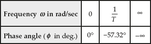
It is clear that for the transportation lag factor, the magnitude plot is zero for all the values of frequency and the phase plot is varying linearly with the frequency .

Table 8.16 shows the different factors with its corner frequency, slope of the magnitude curve, values of the magnitude in dB and phase angle in degrees.

Table 8.16 ∣ Possible factors present in a given system

8.15 Constructing the Bode Plot for a Given System

Consider the loop transfer function as

Substituting , we obtain

Now, the corner frequencies of the given system are

The phase plot is independent of the corner frequency. Since the magnitude of each term present in the transfer function is calculated in the increasing order of corner frequency, the magnitude plot depends on the corner frequency.

Hence, the relation between the corner frequencies is considered as .

8.15.1 Construction of Magnitude Plot

For each term present in the loop transfer function, the slope of the magnitude curve varies. To combine the slope of the different terms present in the given system, the following steps are followed:

1. Slope of each term is calculated.
2. Change in slope from one term to another in the order of increasing corner frequencies has to be determined using Table 8.17. Usually, the constant term along with the pole or zero at the origin is taken as a term.

   Table 8.17 ∣ Determination of change in slope at different corner frequencies

   
3. Two different frequencies other than the corner frequencies are chosen arbitrarily as lower frequency value and higher frequency value such that the relation between different frequencies is

   

4. Determine the gain at different frequencies in increasing order. In this case, there are five different frequencies and have only four terms. Hence, the magnitude of the first term in Table 8.17 is calculated at the first two frequencies. In this case, the magnitude of is calculated at and . The calculation of magnitude at other frequencies and is done using the formula

   Gain at

   where

   The gain at different frequencies are tabulated as given in Table 8.18.

   Table 8.18 ∣ Gain at different frequencies

   
5. Any term in the estimation of magnitude has to be included only after its corresponding corner frequency is crossed.
6. Using Table 8.18, the magnitude plot for the given system can be drawn.

8.15.2 Construction of Phase Plot

The construction of phase plot is much simpler when compared to construction of magnitude plot.

The phase angle of the given system as a function of frequency has to be determined as

for

and for

The values of at different frequencies are calculated including the frequencies mentioned in Table 8.18 and tabulated.

8.16 Flow Chart for Plotting Bode Plot

The flow chart for plotting the Bode plot (both magnitude and phase angle plot) for a given system is shown in Fig. 8.17.

Fig. 8.17 ∣ Flow chart for plotting the Bode plot for a system

8.17 Procedure for Determining the Gain K from the ­Desired Frequency Domain Specifications

The flow chart for determining the gain K for the desired is given in Fig. 8.18(a).

Fig. 8.18 (a) ∣ Determination of K for the desired ω_gc

The flow chart for determining the gain K for the desired is given in Fig. 8.18(b).

Fig. 8.18 (b) ∣ Determination of K for the desired g_m

The flow chart for determining the gain for the desired is shown in ­Fig. 8.18(c).

Fig. 8.18 (c) ∣ Determination of K for the desired p_m

8.18 Maximum Value of Gain

The gain has an effect only on the magnitude plot of a loop transfer function of a system. The magnitude plot of a loop transfer function can be shifted vertically upwards or vertically downwards depending on the gain . If there is an increase in gain value from the original value, then the magnitude plot gets shifted vertically upward and if there is a decrease in gain from the original value, then the magnitude plot gets shifted vertically downward. The gain value cannot be increased or decreased infinitely. There exists some limits in doing so. The gain can be increased or decreased till the magnitude reaches dB at phase crossover frequency. The new gain can be determined as

where is the value by which the magnitude plot has been raised or lowered to reach dB at .

8.19 Procedure for Determining Transfer Function from Bode Plot

The step-by-step procedure for determining the transfer function of a system from its magnitude plot are:

Step 1: Determine the number of corner frequencies existing in the system (the point at which the slope of the system changes). If there exist different slopes for the given system, then there exist different corner frequencies.

Step 2: Determine the initial slope and final slope of the system.

Step 3: Construct a table for the given system in the format given below to determine the different factors present in the system.

Step 4:Determine the gain , corner frequencies, unknown frequencies and unknown magnitude values using the equation of a straight line, , where is the magnitude in dB, is the slope of the line in dB/dec, is the logarithmic value of frequency , i.e., in rad/sec and is the constant.

8.20 Bode Plot for Minimum and Non-Minimum Phase Systems

Consider the loop transfer function of a minimum phase transfer function as

(8.27)

and the loop transfer function of a non-minimum phase system as

(8.28)

where

The pole-zero plots of the minimum and non-minimum systems are shown in Fig. 8.19.

Fig. 8.19 ∣ Pole-zero plots of (a) minimum and (b) non-minimum phase systems

The magnitude and phase angle of the transfer function can be obtained by substituting in Eqs. (8.27) and (8.28) as

and (8.29)

(8.30)

From Eqs. (8.29) and (8.30), it is clear that the magnitudes of minimum phase system and non-minimum phase system are same, whereas the phase angles of minimum phase system and non-minimum phase system are different. The magnitude and phase plots of minimum and non-minimum phase systems are shown in Fig. 8.20.

Fig. 8.20 ∣ Phase plot of minimum and non-minimum phase systems

Solution:

1. The loop transfer function of a system is given by

   

2. Substituting , we obtain

   

3. Two corner frequencies exist in the given loop transfer function are:

   rad/sec and rad/sec.

   To sketch the magnitude plot

4. The change in slope at different corner frequencies are given in Table E8.12(a).

   Table E8.12(a) ∣ Determination of change in slope at different corner frequencies

   
5. Assume the lower frequency as = 1 rad/sec and higher frequency as = 30 rad/sec.
6. The values of gain at different frequencies are determined and given in Table E8.12(b).

   Table E8.12(b) ∣ Gain at different frequencies

   
7. The magnitude plot of the given system is plotted using Table E8.12(b) and is shown in Fig. E8.12(a).

   To sketch the phase plot

8. The phase angle of the given loop transfer function as a function of frequency is obtained as

   

9. The phase angle at different frequencies are obtained by using the above equation and the values are tabulated as given in Table E8.12(c).

   Table E8.12(c) ∣ Phase angle of the system for different frequencies

   
10. The phase plot of the given system is plotted using Table E8.12(c) and is shown in Fig. E8.12(b).

    Hence, the magnitude and phase plots for the loop transfer function of the system are shown in Fig. E8.12.

    

    Fig. E8.12

11. The frequency domain specifications for the given system can be obtained by drawing two horizontal lines across the two plots of the given system (one across the magnitude plot at 0 dB and another across the phase plot at −180°).

    From the definition of gain crossover frequency, phase crossover frequency, gain margin, phase margin and from the graph shown in Fig. E8.12, the frequency domain specifications values are obtained as

    Gain crossover frequency, rad/sec

    Phase crossover frequency, rad/sec

    Gain margin, dB

    Phase margin,

12. The stability of the system can be determined based on either the frequency or the gain.

    Based on frequency:

    Since , the system is stable.

    Based on frequency domain specifications:

    Since the gain margin and phase margin are greater than zero and , the system is stable.

Solution:

1. Given .
2. Substituting and , we obtain

   

3. The two corner frequencies in the given system are

   rad/sec and rad/sec.

   To sketch the magnitude plot

4. The change in slope at different corner frequencies is given in Table E8.13(a).

   Table E8.13(a) ∣ Determination of change in slope at different corner frequencies

   
5. Assume the lower frequency as = 0.1 rad/sec and higher frequency as = 20 rad/sec.
6. The values of gain at different frequencies are determined and given in Table E8.13(b).

   Table E8.13(b) ∣ Gain at different frequencies

   
7. The magnitude plot of the given system is plotted using Table E8.13(b) and is shown in Fig. E8.13(a).

   To sketch the phase plot

8. The phase angle of the given loop transfer function as a function of frequency is obtained as

   

9. The phase angles at different frequencies are tabulated as given in Table E8.13(c).

   Table E8.13(c) ∣ Phase angle of the system for different frequencies

   
10. The phase plot of the given system is plotted using Table E8.13(c) and is shown in Fig. E8.13(a).
    

    Fig. E8.13 (a)

11. The frequency domain specifications for the given system can be obtained by drawing two horizontal lines across the two plots of the given system (one across the magnitude plot at 0 dB and the other across the phase plot at −180°).

    From the definitions of gain crossover frequency, phase crossover frequency, gain margin, phase margin and the graph shown in Fig. E8.13(a), the frequency domain specifications values are obtained as

    Gain crossover frequency, rad/sec

    Phase crossover frequency, rad/sec

    Gain margin, dB

    Phase margin,

12. The next step is to determine the gain corresponding to a particular gain margin and phase margin.

(i) To determine the gain value and gain margin corresponding to desired phase margin:

The required phase margin for the system is .

But it is known that, phase margin .

Therefore, .

Hence, from Fig. E8.13(a), the new gain crossover frequency for a phase angle of is rad/sec.

It is proven that at the gain crossover frequency, the magnitude must be 0 dB. But from Fig. E8.13(a), the magnitude at dB. Hence, the magnitude plot shown in Fig. E8.13(a) is raised by 5dB.

The modified Bode plot is shown in Fig. E8.13(b).

From Fig. E8.13(b), the new frequency domain specifications are

New phase margin,

New gain margin, =16 dB

New gain crossover frequency, 1.3 rad/sec

The value of for the newly obtained Bode plot is determined as

where is the value in dB by which the original magnitude plot has been raised or lowered. In this case, the value of is 5 dB.

Hence,

Therefore, the value of is .

Fig. E8.13 (b)

(ii) To determine the gain and phase margin corresponding to the gain margin

The required gain margin dB.

We know that, the gain margin is obtained using the formula,

Therefore, required is dB.

But for the given system from the Bode plot shown in Fig. E8.13(a), the gain at is dB. Hence, it is clear that every point in the magnitude plot shown in Fig. E8.13(a), has to be reduced by dB. The modified Bode plot is shown in Fig. E8.13(c).

From the Bode plot shown in Fig. E8.13(c), the obtained frequency domain specifications are:

New phase margin,

New gain margin, = 30 dB

The value of for the newly obtained Bode plot is determined as

, where is the value in dB by which the original magnitude plot has been raised or lowered. In this case, the value of is −10.

Hence,

Therefore, the value of is .

Fig. E8.13 (c)

Solution:

1. The loop transfer function of the system is given by .
2. Substituting and in the given system, we obtain

   

3. The two corner frequencies existing in the system are

   rad/sec and rad/sec.

4. The change in slope at different corner frequencies is given in Table E8.14(a).

   Table E8.14(a) ∣ Determination of change in slope at different corner frequencies

   
5. Assume rad/sec and rad/sec.
6. The values of gain at different frequencies are determined and given in Table E8.14(b).

   Table E8.14(b) ∣ Gain at different frequencies

   
7. The magnitude plot of the given system is plotted using Table E8.14(b) and is shown in Fig. E8.14(a).

   To sketch the phase plot

8. The phase angle of the given loop transfer function as a function of frequency is obtained as

   

9. The phase angles at different frequencies are tabulated as given in Table E8.14(c).

   Table E8.14(c) ∣ Phase angle of the system for different frequencies

   
10. The phase plot of the given system is plotted using Table E8.14(c) and is shown in Fig. E8.14(a).
    

    Fig. E8.14 (a)

11. The frequency domain specifications for the given system are:

    Gain crossover frequency, (ω_gc) = 1 rad/sec.

    Phase crossover frequency, ( ω_pc) = 0 rad/sec.

    Gain margin, (g_m) = ∞ dB.

    Phase margin, (p_m) = −50°.

12. The next step is to determine the gain corresponding to a particular gain crossover frequency.

It is given that the required gain crossover frequency of the system is rad/sec, i.e., rad/sec. Hence, it is necessary that the magnitude of the system at must be 0 dB. But from the Bode plot of the system shown in Fig. E8.14(a), the magnitude of the system is 28 dB.

Therefore, each and every point present in the magnitude plot must be added by dB. Hence, the modified Bode plot with rad/sec is shown in Fig. E8.14(b).

Fig. E8.14 (b)

The value of for the new Bode plot is determined as follows:

where is the value by which the magnitude plot has been raised or ­lowered. In this case, dB.

Hence,

Therefore, the = .

Solution:

1. The loop transfer function of the system is .
2. Substituting , we obtain

   

3. The three corner frequencies existing in the system are

   rad/sec, rad/sec and rad/sec.

   To sketch the magnitude plot

4. The change in slope at different corner frequencies is given in Table E8.15(a).

   Table E8.15(a) ∣ Determination of change in slope at different corner frequencies

   
5. Assume rad/sec and rad/sec.
6. The values of gain at different frequencies are determined and given in Table E8.15(b).

   Table E8.15(b) ∣ Gain at different frequencies

   
7. The magnitude plot of the given system is plotted using Table E8.15(b) and is shown in Fig. E8.15.

   To sketch the phase plot

8. The phase angle of the given loop transfer function as a function of frequency is obtained as

   

9. The phase angles at different frequencies are tabulated as given in Table E8.15(c).

   Table E8.15(c) ∣ Phase angle of the system for different frequencies

   
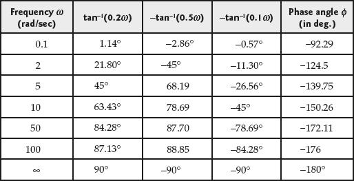
10. The phase plot of the given system is plotted using Table E8.15(c) and is shown in Fig. E8.15.
    

    Fig. E8.15

11. The frequency domain specifications for the given system are:

    Gain crossover frequency, rad/sec

    Phase margin,

    From Table E8.15(c), it is clear that the phase angle of the system becomes only when the frequency of the system is ∞ rad/sec. Hence, phase crossover frequency of the system is ∞ rad/sec. Therefore, the gain margin of the system is also ∞ dB.

12. The stability of the system can be determined based on either the frequency or the gain.

    Based on frequency: Since , the system is stable.

    Based on frequency domain specifications: Since the gain margin and phase margin are greater than zero and , the system is stable.

Solution:

1. The loop transfer function of the given system is .
2. Substituting and rearranging, we obtain

   

3. The three corner frequencies existing in the system are

   rad/sec, rad/sec and the third corner frequency is obtained as ­ follows.

   Comparing the standard second-order characteristic equation with the given quadratic factor, we obtain

   rad/sec and

   Hence, the third corner frequency existing in the system is rad/sec.

   To sketch the magnitude plot

4. The change in slope at different corner frequencies are given in Table E8.16(a).

   Table E8.16(a) ∣ Determination of change in slope at different corner frequencies

   
5. Assume rad/sec and rad/sec.
6. The values of gain at different frequencies are determined and given in Table E8.16(b).

   Table E8.16(b) ∣ Gain at different frequencies

   
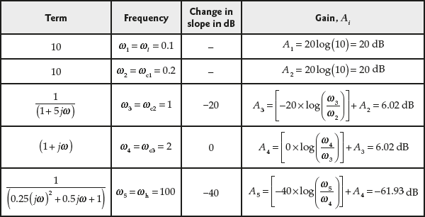
7. The magnitude plot of the given system is plotted using Table E8.16(b) and is shown in Fig. E8.16.

   To sketch the phase plot

8. The phase angle of the given loop transfer function as a function of frequency is obtained as

   

9. The phase angles at different frequencies are tabulated as given in Table E8.16(c).

   Table E8.16(c) ∣ Phase angle of the system for different frequencies

   
10. The phase plot of the given system is plotted using Table E8.16(c) and is shown in Fig. E8.16.
    

    Fig. E8.16

11. The frequency domain specifications are:

    Gain crossover frequency, 2.8 rad/sec

    Phase crossover frequency, rad/sec

    Gain margin, dB

    Phase margin,

Solution:

1. The loop transfer function of the given system is
2. Substituting and rearranging, we obtain

   

3. The two corner frequencies existing in the system are

   rad/sec and rad/sec.

   To sketch the magnitude plot

4. The change in slope at different corner frequencies is given in Table E8.17(a).

   Table E8.17(a) ∣ Determination of change in slope at different corner frequencies

   
5. Assume rad/sec and rad/sec.
6. The values of gain at different frequencies are determined and given in Table E8.17(b).

   Table E8.17(b) ∣ Gain at different frequencies

   
7. The magnitude plot of the given system is plotted using Table E8.17(b) and is shown in Fig. E8.17.

   To sketch the phase plot

8. The phase angle of the given loop transfer function as a function of frequency is obtained as

   .

9. The phase angles at different frequencies are tabulated as given in Table E8.17(c).

   Table E8.17(c) ∣ Phase angle of the system for different frequencies

   
10. The phase plot of the given system is plotted using Table E8.17(c) and is shown in Fig. E8.17.
    

    Fig. E8.17

11. The frequency domain specifications of the system are:

    Gain crossover frequency, rad/sec

    Phase crossover frequency, rad/sec

    Gain margin, dB

    Phase margin,

Solution:

1. The loop transfer function of the given system is .
2. Substituting , we obtain
3. It is known that for a simple zero, the slope is dB/dec and there exists no corner frequency for the given system. Hence, for the given system the slope is .
4. As there exists only one factor in the given system, the change in slope cannot be determined.
5. The magnitude for the given system is
6. The phase angle for the given system is

Hence, the magnitude and phase plots for the given system depends on .

Table E8.19 ∣ Frequency response of a system

Determine (a) gain margin and phase margin of the system and (b) change in gain so that the gain margin of the system is dB.

Solution:

1. From Table E8.19, the frequency domain specifications are:

   Gain crossover frequency, rad/sec

   Phase crossover frequency, rad/sec

   Gain margin, dB

   Phase margin,

2. For the gain , the gain margin dB. But the required gain margin is dB. Therefore, the magnitude at different frequency should increase by dB.

   Hence,

   i.e., .

   Therefore, change in gain required to have the gain margin of the system as dB is .

Solution:

1. The loop transfer function of the given system is

   

2. Rearranging the above equation, we obtain

   

3. The three corner frequencies existing in the system are rad/sec, rad/sec and the third corner frequency is obtained as follows.

   Comparing the standard second-order characteristic equation with the given quadratic factor, we obtain

   rad/sec and

   Hence, the third corner frequency existing in the system is rad/sec.

   To sketch the magnitude plot

4. The change in slope at different corner frequencies is given in Table E8.20(a).

   Table E8.20(a) ∣ Determination of change in slope at different corner frequencies

   
5. Assume rad/sec and rad/sec.
6. The values of gain at different frequencies are determined and given in Table E8.20(b).

   Table E8.20(b) ∣ Gain at different frequencies

   
7. The magnitude plot of the given system is plotted using Table E8.20(b) and is shown in Fig. E8.20.

   To sketch the phase plot

8. The phase angle of the given loop transfer function as a function of frequency is obtained as

   

9. The phase angles at different frequencies are tabulated as given in Table E8.20(c).

   Table E8.20(c) ∣ Phase angle of the system for different frequencies

   
10. The phase plot of the given system is plotted using Table E8.20(c) and is shown in Fig. E8.20.
    

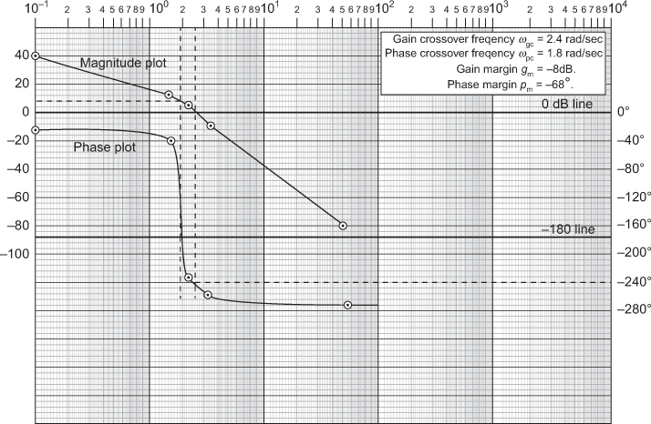
    Fig. E8.20

11. The frequency domain specifications for the system are:

    Gain crossover frequency, rad/sec

    Phase crossover frequency, rad/sec

    Gain margin, dB

    Phase margin,

Solution:

1. The loop transfer function of the given system is
2. Substituting , we obtain

   

3. The corner frequency that exists in the system is rad/sec

   To sketch the magnitude plot

4. The change in slope at different corner frequencies is given in Table E8.21(a).

   Table E8.21(a) ∣ Determination of change in slope at different corner frequencies

   
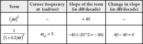
5. Assume rad/sec and rad/sec.
6. The values of gain at different frequencies are determined and given in Table E8.21(b).

   Table E8.21(b) ∣ Gain at different frequencies

   
7. The magnitude plot of the given system is plotted using Table E8.21(b) and is shown in Fig. E8.21.

   To sketch the phase plot

8. The phase angle of the given loop transfer function as a function of frequency is obtained as

   =

9. The phase angle at different frequencies are tabulated as given in Table E8.21(c).

   Table E8.21(c) ∣ Phase angle of the system for different frequencies

   
10. The phase plot of the given system is plotted using Table E8.21(c) and is shown in Fig. E8.21.
    

    Fig. E8.21

11. The frequency domain specifications of the system are:

    Gain crossover frequency, rad/sec

    Phase crossover frequency, rad/sec

    Gain margin, dB

    Phase margin,

Solution:

1. The loop transfer function of the given system is
2. As the roots of the quadratic factor are real, we can split the quadratic factor as

   

3. Substitute and rearranging, we obtain

   

   =

4. The four corner frequencies existing in the system are

   rad/sec, rad/sec, rad/sec and

   rad/sec.

   To sketch the magnitude plot

5. The change in slope at different corner frequencies is given in Table E8.22(a).
6. Assume rad/sec and rad/sec.

   Table E8.22(a) ∣ Determination of change in slope at different corner frequencies

   
7. The values of gain at different frequencies are determined and given in Table E8.22(b).

   Table E8.22(b) ∣ Gain at different frequencies

   
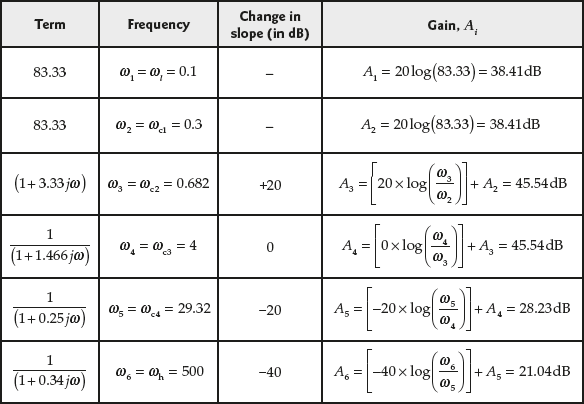
8. The magnitude plot of the given system is plotted using Table E8.22(b) and is shown in Fig. E8.22.
   

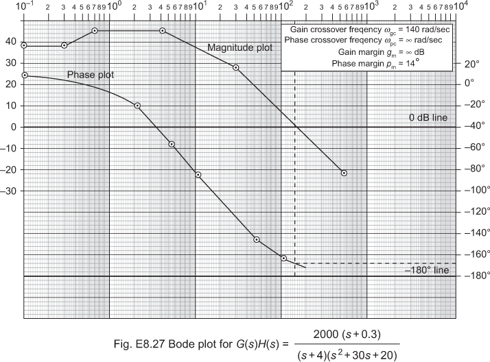
   Fig. E8.22

   To sketch the phase plot

9. The phase angle of the given loop transfer function as a function of frequency is obtained as

   

10. The phase angles at different frequencies are tabulated as given in Table E8.22(c).

    Table E8.22(c) ∣ Phase angle of the system for different frequencies

    
11. The phase plot of the given system is plotted using Table E8.22(c) and is shown in Fig. E8.22.
12. The frequency domain specifications of the given system are:

    Gain crossover frequency, rad/sec

    Phase crossover frequency, rad/sec

    Gain margin, dB

    Phase margin,

Solution:

1. The loop transfer function of the given system is
2. Substituting and and rearranging, we obtain

   

   where .

3. The two corner frequencies existing in the system are

   rad/sec and rad/sec.

   To sketch the magnitude plot

4. The change in slope at different corner frequencies is given in Table E8.23(a).

   Table E8.23(a) ∣ Determination of change in slope at different corner frequencies

   
5. Assume rad/sec and rad/sec.
6. The values of gain at different frequencies are determined and given in Table E8.23(b).

   Table E8.23(b) ∣ Gain at different frequencies

   
7. It is known that the delay term () present in the loop transfer function will ­contribute only to phase angle plot. Hence, the magnitude plot of any system with or without delay terms is same.
8. The magnitude plot of the given system is plotted using Table E8.23(b) and is shown in Fig. E8.23.

   To sketch the phase plot

9. The phase angle of the given loop transfer function as a function of frequency is obtained as

   

   =

10. The phase angles at different frequencies are tabulated as given in Table E8.23(c).

    Table E8.23(c) ∣ Phase angle of the system for different frequencies

    
11. The phase plot of the given system is plotted using Table E8.23(c) and is shown in Fig. E8.23.
    

    Fig. E8.23

12. The frequency domain specifications of the system are:

    Gain crossover frequency, rad/sec

    Phase crossover frequency, rad/sec

    Gain margin, dB

    Phase margin,

Fig. E8.24(a)

Solution:

1. The loop transfer function of the system shown in Fig. E8.24(a) is .
2. Substituting and and rearranging, we obtain

   

3. The three corner frequencies existing in the system are

   rad/sec, rad/sec and rad/sec.

   To sketch the magnitude plot

4. The change in slope at different corner frequencies is given in Table E8.24(a).

   Table E8.24(a) ∣ Determination of change in slope at different corner frequencies

   
5. Assume rad/sec and rad/sec.
6. The values of gain at different frequencies are determined and given in Table E8.24(b).

   Table E8.24(b) ∣ Gain at different frequencies

   
7. The magnitude plot of the given system is plotted using Table E8.24(b) and is shown in Fig. E8.24(b).
   

   Fig. E8.24(b)

   To sketch the phase plot

8. The phase angle of the given loop transfer function as a function of frequency is obtained as

   

9. The phase angles at different frequencies are tabulated as given in Table E8.24(c).

   Table E8.24(c) ∣ Phase angle of the system for different frequencies

   
10. The phase plot of the given system is plotted using Table E8.24(c) and is shown in Fig. E8.24(b).
11. The frequency domain specifications of the system are:

    Gain crossover frequency, rad/sec

    Phase crossover frequency, rad/sec

    Gain margin, dB

    Phase margin,

    To determine the maximum gain

12. The magnitude in dB at is 37 dB. Therefore, the magnitude plot can be raised by dB until the magnitude becomes dB at . Therefore, the maximum gain is determined as

    

    

Solution:

1. The loop transfer function of the given system is
2. Substituting , we obtain

   

3. The two corner frequencies existing in the system are

   rad/sec and .

   To sketch the magnitude plot

4. The change in slope at different corner frequencies is given in Table E8.25(a).

   Table E8.25(a) ∣ Determination of change in slope at different corner frequencies

   
5. Assume rad/sec and rad/sec.
6. The values of gain at different frequencies are determined and given in Table E8.25(b).

   Table E8.25(b) ∣ Gain at different frequencies

   
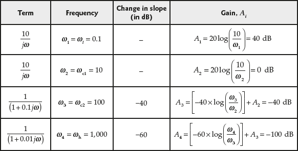
7. It is known that the delay term () present in the loop transfer function will ­contribute only to the phase angle plot. Hence, the magnitude plot of any system with or without delay term is same.
8. It is clear from Table E8.25(b) that the gain crossover frequency is rad/sec.
9. The phase angle of the system is

   (1)

10. To determine the maximum value of time delay, :

    The phase margin for the system to be stable is . Therefore,

    

Substituting Eqn. (1) in the above equation, we obtain

Substituting = 10 rad/sec, we obtain

i.e., T = 0.068 sec.

Therefore, maximum time delay, , for the closed-loop system to be stable is sec.

Fig. E8.26 (a)

Solution:

From Fig. E8.26(a), we can obtain the following information:

1. Three corner frequencies exist in the system
2. Initial slope of the plot = dB/decade
3. Final slope of the plot = dB/decade

The change in slope from initial to final slope occurs in three steps and the factor that could be present in the transfer function for that change in slope to occur is given in Table E8.26.

Table E8.26 ∣ Factor for the change in slope

Therefore, from the above table, we can determine the loop transfer function of the system as a function of gain value as

The values of time constants and can be determined from their respective corner frequencies as

, and .

Hence, the loop transfer function of the system as a function of is

To determine the gain K

The gain can be determined using the general equation of straight line, i.e., where is the magnitude of in dB, is the slope of the line, is the logarithmic frequency in and is the constant.

The given magnitude plot of a system is redrawn as shown in Fig. E8.26(b).

Fig. E8.26(b)

For the line segment , we have

Slope of the line, .

Therefore,

At dB.

Therefore, i.e., c =32.

The magnitude at is

Solving the above equation, we obtain dB.

At rad/sec, only the gain and poles at the origin exist in the system, i.e., .

Therefore,

Therefore, .

Hence, the transfer function for the given magnitude plot of a system is

Fig. E8.27 (a)

Solution:

From Fig. E8.27(a), we can obtain the following information:

1. Three corner frequencies exist in the system
2. Initial slope of the plot = 0 dB/decade
3. Final slope of the plot = dB/decade

The change in slope from initial to final slope occurs in three steps and the factor that could be present in the transfer function for that change in slope to occur is given in Table E8.27.

Table E8.27 ∣ Factor for the change in slope

Therefore, from Table E8.27, we can determine the loop transfer function of the system as a function of gain value as

To determine the gain K and corner frequencies:

1. As the initial slope of the magnitude plot is dB/decade and the magnitude is dB, we obtain the gain as

   

   Therefore,

2. Corner frequencies

   The gain can be determined using the general equation of straight line, i.e., where is the magnitude of in dB, is the slope of the line, is the logarithmic frequency in and is the constant.

   The magnitude plot given in Fig. E8.27(a) can be redrawn as shown in Fig. E8.27(b).

   

   Fig. E8.27 (b)

For the line segment , we have

Therefore,

At , dB.

Therefore,

Solving the above equation, we obtain

Also, at , dB

Therefore,

Solving the above equation, we obtain s.

Similarly, for line segment , we have

Therefore,

At , dB.

Therefore,

Solving the above equation, we obtain

Also, at , dB

Therefore,

Solving the above equation, we obtain s.

Similarly, for line segment , we have

Therefore,

At , dB.

Therefore,

Solving the above equation, we obtain

Also, at , dB

Therefore,

Solving the above equation, we obtain s.

Therefore, the required transfer function will be

Review Questions

1. Define frequency response of a system and discuss about the advantages of frequency response method for the analysis of linear systems.
2. Discuss the correlation between frequency response and transient response for a second-order system. Derive any expression used.
3. Explain the procedure to get the closed-loop frequency response from the loop transfer function.
4. Explain the procedure for experimentally determining the frequency response of an electric circuit containing several interconnected components. Draw a complete schematic diagram of the experimental set-up.
5. What are the different methods available for frequency response plot?
6. Discuss the advantages of frequency response analysis over the root locus technique.
7. Write down the frequency domain specifications.
8. Define the frequency domain specification for bandwidth.
9. What are the advantages and disadvantages of having large bandwidth?
10. Express the resonant peak M_p and the resonant frequency in terms of natural ­frequency of oscillation and damping ratio for a unity feedback second-order system.
11. If a control system is required to have a given value for the resonant peak, describe how you would get the required value of the static loop gain , given the loop transfer ­function.
12. Explain the effect of feedback on the gain and bandwidth of the system.
13. What do you understand by frequency response plot?
14. What are the unique features of Bode plots?
15. What is corner frequency in Bode plot?
16. Define minimum phase transfer function.
17. Explain the gain margin and phase margin.
18. Define gain and phase crossover frequencies.
19. Explain the significance of phase margin and gain margin in determining the relative stability of closed-loop systems.
20. What are the advantages and disadvantages of Bode plot?
21. What is the major difference between Bode magnitude plots for first-order system and second-order system?
22. Describe the change in open-loop frequency response magnitude plot if the time delay is added to the plant.
23. If the phase response of a pure time delay is plotted on a linear phase versus linear frequency plot, what would be the shape of the curve?
24. What will be initial slope of the Bode magnitude plot for a system having no poles and no zeros at origin?
25. Tabulate the phase angle versus frequency for the loop transfer function of a system given by .
26. A second-order system has a natural frequency of oscillation rad/sec and damped frequency of oscillation rad/sec. Determine (i) when it is subjected to a step input, calculate its percentage overshoot and (ii) when it is subjected to a sinusoidal input, calculate the maximum ratio to its output (resonant peak).
27. An under damped second-order system exhibited 17% overshoot for a step input, and the frequency of oscillations was 0.5 Hz. Calculate the resonant peak M_p and the resonant frequency of the frequency response of this system.
28. A closed-loop transfer function of an automatic control system is given by

    

    Calculate (i) the peak response and resonant frequency of the system and (ii) damping ratio and natural frequency of oscillation of the equivalent second-order system.

29. The overshoot of the unit step response of a second-order feedback system is 30 per cent. Determine (a) damping ratio , (b) resonant peak , (c) resonant frequency , (d) damping frequency and (e) time at which peak overshoot occurs. Assume natural frequency of oscillation rad/sec.
30. Determine the bandwidth for the closed-loop transfer function given by

    

31. The transfer function of a system is given by . Show that .
32. The closed-loop transfer function of a unity feedback control system is . The peak overshoot for a unit step input is 25 per cent. The damped frequency of oscillation is rad/sec. Determine , bandwidth and the time at which the first overshoot occurs. In addition, find the steady state error of the system if .
33. For if and rad/sec, determine and and hence calculate the settling time and bandwidth.
34. A control system is represented by Fig. Q8.34.
    

    Fig. Q8.34

    Determine (i) the values of and so that and rad/sec and (ii) corresponding bandwidth.

35. The transfer function of a system is given by . (a) When  , determine the maximum time delay in seconds for the closed-loop system to be stable and (b) when sec determine the maximum gain for the system to be stable.
36. For a unity feedback system shown in Fig. Q8.36, determine (a) , (b) and (c) bandwidth of the system for and .
    

    Fig. Q8.36

37. Consider a unity feedback system whose loop transfer function is  . ­Determine gain such that the resonant peak magnitude in the ­frequency response is 2 dB or dB.
38. A unit step input is applied to a feedback control system whose open-loop transfer function is given by Determine and given that maximum overshoot is 26 per cent and resonant frequency is rad/sec. Calculate resonance peak , gain crossover frequency and phase margin.
39. For each closed-loop system with the following performance characteristics, determine the closed-loop bandwidth for (a) , (b) , (c) and (d) .
40. Determine the resonant frequency , resonant peak and bandwidth for the system whose transfer function is given by .
41. Determine the phase crossover frequency, gain crossover frequency, gain margin and phase margin for the given system with and without ­plotting the Bode plot. Also comment on the stability of the stability.
42. Determine analytically the gain margin and phase margin for the system with the ­following transfer function . Also determine the gain crossover frequency and phase cross over frequency.
43. The transfer function of an electric circuit is . Determine (a) gain margin and phase margin and (b) gain and phase angle at a frequency of 1 kHz.
44. An amplifier is subjected to a sinusoidal voltage gain as . Determine the amplitude of output signal and the phase difference between output and input. The amplifier transfer function is .
45. A sinusoidal waveform is fed to a constant block with a transfer function of 0.675. Determine (a) signal gain, (b) output amplitude and (c) phase difference between input and output.
46. The loop transfer function of a system is given by . Sketch the Bode plot for the given system. Also, determine the frequency domain specifications.
47. The loop transfer function of a system is given by . Sketch the Bode plot for the given system and determine the frequency domain specifications.
48. The loop transfer function of a system is given by  . Sketch the Bode plot for the given system and determine the frequency domain ­specifications.
49. The loop transfer function of a system is given by . Sketch the Bode plot for the given system and determine the frequency domain specifications.
50. The loop transfer function of a system is given by . Sketch the Bode plot for the given system and determine the frequency domain specifications.
51. The loop transfer function of a system is given by . Sketch the Bode plot for the given system and determine the frequency domain specifications.
52. The loop transfer function of a system is given by  . Sketch the Bode plot for the given system and determine the frequency domain ­specifications.
53. The loop transfer function of a system is given by  . Sketch the Bode plot for the given system and determine the frequency domain specifications.
54. The loop transfer function of a system is given by . Sketch the Bode plot for the given system and determine the frequency domain specifications.
55. The loop transfer function of a system is given by  . Sketch the Bode plot for the given system and determine the frequency domain specifications.
56. Determine the gain and phase margins of the system using Table Q8.56.

    Table Q8.56

    
57. The loop transfer function of a system is . Determine the gain margin and phase margin using Bode plot.
58. A constant block has a magnitude of 20 dB at 100 rad/sec. Determine (a) block transfer function, (b) magnitude at a frequency of 1,000 rad/sec and (c) phase angle at 1,000 rad/sec.
59. Determine the stability of the system using Bode plot whose block diagram is given in Fig. Q8.59.
    

    Fig. Q8.59

60. A unity feedback control system is characterized by an open-loop transfer function

    .

    Show that the gain margin of the system is

61. A negative feedback control system is characterized by an open-loop transfer function . Determine (a) for a gain margin of 10 dB, (b) for a of 30 dB, (c) K to give phase margin of 24° and (d) the marginal value of for stability.
62. At the phase crossover frequency, the gain of the system is . What is the corresponding gain margin in dB?
63. The block diagram of a floppy disc is shown in Fig. Q8.64.
    

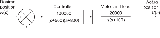
    Fig. Q8.64

    Use frequency response technique to determine (a) , zero dB frequency 180^° frequency, (b) closed-loop bandwidth, percentage overshoot, settling time and peak time and also comment on the stability of the system.

64. Draw the Bode plot for the transfer function
65. The open-loop transfer function of a unity feedback system is given by

    .

    Derive an expression for gain K in terms of and specified gain margin .

66. For the given transfer function sketch the Bode magnitude and phase angle plot. Obtain gain margin and phase margin.
67. The loop transfer function of a system is given by . Sketch the Bode plot for the given system. Also, determine the gain K when the gain margin is 10 dB.
68. The loop transfer function of a system is given by . Sketch the Bode plot for the given system. Also, determine the gain K when the phase margin is 30°.
69. The loop transfer of a given system is given by . Sketch the Bode plot for the given system. Also, determine the gain margin and phase margin of the system.
70. The loop transfer function of a system is given by  . Sketch the Bode plot for the given system and determine the frequency domain specifications.
71. A servo control system of type 0, has a transfer function . Sketch the Bode plot and comment on the stability of the system.
72. Explain the Bode plot for the following functions of a unity feedback system.

    (i) (ii) and (iii)

73. Explain the Bode plot for the following functions of a unity feedback system:

    (i) and (ii)

74. The closed-loop control system incorporating an amplifier with a gain of K is shown in Fig. Q8.75.
    

    Fig. Q8.75

    Using Bode plot, determine (a) is the system stable for a gain K = 1 and (b) what is the maximum value of K before the system becomes unstable.

75. Draw the Bode plot for the system shown in Fig. Q8.76. Determine (i) and (ii) whether the closed-loop system is stable (iii) obtain the closed-loop frequency response and plot on a Bode diagram. Find the resonance frequency and bandwidth. What are the ­values of and settling time?
    

    Fig. Q8.76

76. Sketch the Bode plot for the loop transfer function . Determine the maximum value of for the system to be stable.
77. Draw the Bode plot for the transfer function where .
78. For the following transfer function, identify the corner frequencies, the initial slope and the final slope of the magnitude plot
79. Consider a system as shown in Fig. Q8.80.
    

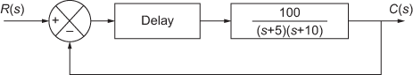
    Fig. Q8.80

    Determine (a) phase margin for the time delay of 0, 0.1, 0.2, 0.5 and 1 s (b) gain margin for the time delay mentioned in (a), (c), for what time delay mentioned in (a), the system is stable and (d) for each time delay that makes the system unstable, how much reduction in gain is required for the system to be stable?

80. The open-loop transfer function of a unity feedback system is  . ­Using Bode plot, determine (a) so that the is 20 dB, (b) so that the is 60° and (c) so that the resonant peak of the system is 1 dB. What are the corresponding values of and and (d) so that the bandwidth of the system is 1.5 rad/sec.
81. Describe the asymptotic phase response of a system with a single pole at −2.
82. For a system with three poles at −4, what is the maximum difference between the asymptotic approximation and the actual magnitude response?
83. The loop transfer function of a system is given by . Sketch the Bode plot for the following two cases: (i) and (ii).
84. Consider a system as shown in Fig. Q8.85. Determine the loop transfer function and sketch the Bode diagram for the same. Also, determine the value of gain such that the phase margin is . What is the gain margin of this system with this gain ?
    

    Fig. Q8.85

85. The block diagram of a control system is shown in Fig. Q8.86. Determine the range of the gain for stability.
    

    Fig. Q8.86

86. Determine the gain margin, phase margin, damping factor and critical ­frequency of ­oscillation for the system with unity feedback and has a transfer function .
87. Sketch the Bode plot for the loop transfer function of the system

    .

    Determine the range of K for closed-loop stability.

88. Determine the gain and phase angle of the system at a frequency of 1 rad/sec. The transfer function of the system is G(s) = (s + 1).
89. The transfer function of the system is given by . Determine the frequency response of the system over a frequency range of 0.1₧10 rad/sec.
90. Determine the gain and phase angle of the given system at a frequency of 0.1 Hz. The transfer function of the system is .