10

CONSTANT M- AND N-CIRCLES AND NICHOLS CHART

10.1 Introduction

The frequency-response techniques discussed in the previous chapters are the open-loop frequency plots that have obtained the information about the closed-loop stability using the open-loop frequency response of the system. In these methods, the frequency response of the loop transfer function is plotted and information regarding the closed-loop stability is derived from the plot. In this chapter, constant M-circles (magnitude), ­constant N-circles (phase) and Nichols chart are discussed, which directly give the information regarding the closed-loop stability of the system.

10.2 Closed-Loop Response from Open-Loop Response

The closed-loop transfer function of a system with open-loop transfer function and feedback transfer function is

Substituting in the above equation, we obtain

Letting , we obtain

(10.1)

where is the magnitude of the closed-loop transfer function and is the phase angle of the closed-loop transfer function.

Since the magnitude and phase angle of the closed-loop system are the function of frequency , the closed-loop frequency plot of a system is the plot of magnitude and phase angle of the closed-loop system with respect to frequency . Analytically or graphically, the ­magnitude and phase angle of the closed-loop system for different values of can be calculated. In ­analytical method, tedious calculations are involved in determining the magnitude and phase angle of the closed-loop system for different values of . The graphical methods that eliminate the disadvantages of the analytical method are constant M- and N-circles and Nichols chart.

10.3 Constant M-Circles

Let the open-loop transfer function of the system be . In frequency-response analysis, is replaced with . Therefore,

(10.2)

where is the real part of and is the imaginary part of .

The closed-loop transfer function of the system with unity feedback is obtained as

Substituting Eqn. (10.2) and using Eqn. (10.1) in the above equation, we obtain

The magnitude of the above equation is

Squaring both sides of the above equation and cross multiplying, we obtain

(10.3)

Simplifying the above equation, we get

i.e.,

Dividing the above equation by , we obtain

Adding the term on both sides of the above equation, we obtain

Upon simplifying, we obtain

i.e., , (10.4)

Equation (10.4) resembles the equation of a circle with centre and radius

The constant M-loci or constant M-circles are the family of circles described by Eqn. (10.4) in -plane when takes different values. The constant M-loci or constant M-circles for different values of are shown in Fig. 10.1.

The following three cases can be inferred from Fig. 10.1.

Fig. 10.1 ∣ Constant M-circles or constant M-loci

Case 1: M > 1

When the magnitude increases, the radius of -circles decreases and the centre of the -circles move towards the point . Therefore, when , the radius of -circle is zero and centre is at . This implies that the constant -circle at ­represents the point . These circles lie to the left of the circle.

Case 2: M = 1

When the magnitude is equal to 1, the radius of -circle is infinity and the centre of the -circle is . This implies that the constant -circles at represents a straight line parallel to imaginary axis and the intersection of the parallel line with the real axis can be determined by substituting in Eqn. (10.3). Thus, the intersection point of circle in the real axis is at .

Case 3: M < 1

When the magnitude decreases, the radius of -circles decreases and the centre of the -circles moves towards the origin. Therefore, when , the radius of -circles is zero and centre is at origin. This implies that the constant -circles at represents the origin.

The above three cases can be explained more clearly with the help of Table 10.1 which gives the centre and radius of -circles for different values of

Table 10.1 ∣ Centre and radius of M-circles

10.3.1 Applications of Constant M-Circles

1. The constant M-circles can be used to determine resonant peak .
2. The resonant frequency can be determined by using the constant M-circles.
3. The gain K of open-loop transfer function with unity feedback system for a desired can be determined.
4. The magnitude plot of the system can be determined easily using constant M-circles.

10.3.2 Resonant Peak M_r and Resonant Frequency ω_r from Constant M-Circles

The polar plot of a loop transfer function and the constant M-circles for the same system are shown in Fig. 10.2.

Fig. 10.2 ∣ Polar plot and constant M-circles

The resonant peak and resonant frequency of the system are determined by using the following steps:

Step 1:The polar plot and constant M-circles for different values of M are drawn as shown in Fig. 10.2.

Step 2:The polar plot will intersect the constant M circles at more than one point.

Step 3:The frequency corresponding to the different intersection points is determined.

Step 4:The circles at which the polar plot is a tangent to the circle are determined and the corresponding M values are found.

Step 5:The value of M with smaller value is the resonant peak of the system.

Step 6:The frequency corresponding to the particular intersection point is the ­resonant frequency of the system .

For the polar plot and the constant M-circles shown in Fig. 10.2, the resonant peak is at and the resonant frequency is .

The flow chart for determining and from constant M-circles is shown in Fig. 10.3.

Fig. 10.3 ∣ Flow chart for determining M_r and ω_r

10.3.3 Variation of Gain K with M_r and ω_r

The variation of gain K with the polar plot is shown in Fig. 10.4. It is evident that as the gain K increases, the values of resonant peak and resonant frequency will also increase.

Fig. 10.4 ∣ Polar plot and constant M-circles for different values of gain K

10.3.4 Bandwidth of the System

When the variation of magnitude of the system with respect to frequency alone is plotted as shown in Fig. 10.5, the bandwidth of the system can be calculated and this is depicted in Fig. 10.5.

Fig. 10.5 ∣ Magnitude versus curve

Also, the resonant peak and resonant frequency are also shown in Fig. 10.5.

10.3.5 Stability of the System

The variation of resonant peak and resonant frequency with respect to variation in gain K is shown in Fig. 10.4. It is clear that, at gain , the resonant peak is . At this point, the system becomes marginally stable. Also, the system will be unstable when its gain is greater than .

10.3.6 Determination of Gain K Corresponding to the Desired Resonant Peak (M_r)_desired

The step-by-step procedure to determine the value of gain K corresponding to the desired resonant peak is given below:

Step 1:The polar plot of the system is drawn by assuming gain .

Step 2:The angle is determined by using the formula, .

Step 3:A radial line OA is drawn from the origin as shown in Fig. 10.6(a).

Step 4:The constant M-circle with with centre on the negative real axis is drawn, which is tangent to both the radial line OA and polar plot as shown in Fig. 10.6(a).

Step 5:Let the constant M-circle touch the radial line OA at B.

Step 6:A perpendicular line is drawn from the point B so that the line intersects the ­negative real axis at C.

Step 7:Thus, the desired gain K is obtained using the formula, .

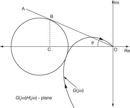
Fig. 10.6(a) ∣ Gain K corresponding to

The flow chart for determining gain for desired resonant peak is given in Fig. 10.6(b).

Fig. 10.6(b) ∣ Flow chart for determining gain K for

10.3.7 Magnitude Plot of the System from Constant M-Circles

The step-by-step procedure for determining the magnitude plot of the system using constant M-circles is given below:

Step 1:The polar plot of a system for the given gain is plotted in -plane.

Step 2:The constant M-circles for different values of M are plotted in the same -plane.

Step 3:The intersection points of the polar plot and constant M-circles are noted down.

Step 4:The frequency corresponding to an intersection point is noted down from polar plot and the magnitude corresponding to the intersection point is the value of M.

Step 5:Once the value of M and its corresponding frequency are noted down from the intersection points, the magnitude plot of the system is obtained by taking the value of M along Y-axis and corresponding frequency along X-axis.

The constant M-circles with polar plot of a system and its corresponding magnitude plot are shown in Figs. 10.7 and 10.8(a) respectively.

Fig. 10.7 ∣ Polar plot and constant M-circles

Fig. 10.8(a) ∣ Magnitude plot of the system

The flow chart for the determination of magnitude plot from constant M-circles is shown in Fig. 10.8(b).

Fig. 10.8(b) ∣ Flow chart for obtaining the magnitude plot from constant M-circles

10.4 Constant N-Circles

Let the open-loop transfer function of the system be . In the frequency response analysis of the system s is replaced with . Therefore,

(10.5)

where u is the real part of and v is the imaginary part of .

The closed-loop transfer function of the system with unity feedback is obtained as

Substituting Eqn. (10.5) and using Eqn. (10.1) in the above equation, we obtain

The phase angle of the system is

Taking tan on both sides of the above equation, we obtain

Substituting in the above equation, we obtain

Using the formula in the above equation, we obtain

Simplifying the above equation, we obtain

Therefore,

Adding on both sides of the above equation, we obtain

Rearranging the above equation, we obtain

(10.6)

The above equation resembles the equation of a circle with centre and radius .

It is to be noted that irrespective of the value of N, Eqn. (10.6) gets satisfied for and . Therefore, each constant N-circle will pass through the origin and in the -plane.

The constant N-loci or constant N-circles are the family of circles described by Eqn. (10.6) in -plane when takes different values. The constant N-loci or constant N-circles for different values of are shown in Fig. 10.9.

The centre and radius of constant N-circles for different values of N are shown in Table 10.2.

Table 10.2 ∣ Centre and radius of N-circles

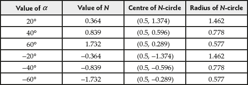
The constant N-circles shown in Fig. 10.9 for a given value of are only arc and not entire circles. Thus constant N-circles for Φ = 60° and Φ = 60° − 180° = −120° are parts of same circle.

Fig. 10.9 ∣ Constant N-circles or constant N loci

10.4.1 Phase Plot of the System from Constant N-Circles

The step-by-step procedure for determining the phase plot of the system using constant N-circles is given below:

Step 1:The polar plot of a system for the given gain is plotted in -plane.

Step 2:The constant N-circles for different values of are plotted in the same -plane.

Step 3:The intersection points of the polar plot and constant N-circles are noted down.

Step 4:The frequency corresponding to an intersection point is noted down from polar plot and the magnitude corresponding to the intersection point is the value of .

Step 5:Once the value of and its corresponding frequency are noted down from the ­intersection points, the magnitude plot of the system is obtained by taking the value of along Y-axis and corresponding frequency along X-axis.

The phase plot for the system using constant N-circles is shown in Fig. 10.10(a).

Fig. 10.10(a) ∣ Phase angle plot of the system

The flow chart for determining the phase angle plot from constant N-circles is shown in Fig. 10.10(b).

Fig. 10.10(b) ∣ Flow chart for plotting phase angle plot of the system

10.5 Nichols Chart

The chart that results after the transformation of constant M- and N-circles to log-magnitude and phase angle coordinates is called Nichols chart. This transformation is first introduced by N.B. Nichols. In addition, the Nichols chart can be defined as the chart that consists of constant M- and N-circles superimposed on a graph sheet. The graph sheet consists of ­magnitude of the system in decibels which is obtained from constant M-circles along the Y-axis and phase angle of the system in degrees which is obtained from constant ­N-circles along the X-axis. The typical Nichols chart with constant M- and N-circles is shown in Fig. 10.11.

Fig. 10.11 ∣ Nichols chart

10.5.1 Reason for the Usage of Nichols Chart

The reason for using Nichols chart for determining the stability of the system is due to the disadvantages that exist in working with the polar coordinates. The disadvantage is that when the loop gain of the system is changed, the polar plot will tend to change its shape. But in Bode plot or in magnitude versus phase plot, when the loop gain of the system is altered, the curve gets shifted up or down vertically. Therefore, it is convenient to work with Nichols chart compared to polar plot.

10.5.2 Advantages of Nichols Chart

The advantages of Nichols chart are:

1. The magnitude and phase plot of the system can be obtained.
2. The values of resonant peak, resonant frequency and bandwidth can be obtained from the Nichols chart for the given .
3. The various time-domain specifications can be obtained once the value of resonant peak and resonant frequency are determined.
4. The gain of the system for the desired resonant peak can be determined.

10.5.3 Transformation of Constant M- and N-Circles into Nichols Chart

The transformation of constant M-circle into Nichols chart is explained using the step- by-step procedure as follows:

Step 1:The constant M-circles for M > 1 are plotted in Fig. 10.12(a).

Fig. 10.12(a) ∣ Constant M-circles of a system

Step 2:A line is drawn from the origin to any point on the constant M-circles as shown in Fig. 10.12(b).

Fig. 10.12(b) ∣ Line from origin to constant M-circles

Step 3:Consider a point A in the constant M-circles.

Step 4:The magnitude in dB and phase angle in degrees for that particular point are

Magnitude in dB =

Phase angle in degrees =

where is the length of the line OA and is the angle from the positive real axis to the line OA taken in the counterclockwise direction.

Step 5:Similarly, any point in the constant M-circles can be plotted in the Nichols chart.

Step 6:The constant M-circles shown in Fig. 10.12(a) are transformed to Nichols chart as shown in Fig. 10.12(c).

Fig. 10.12(c) ∣ Constant M circle in Nichols chart

It is noted that the critical point is plotted in Nichols chart as the point .

Similarly, the constant N-circles can be transformed into Nichols chart.

10.5.4 Determination of Frequency Domain Specifications from Nichols Chart

The different frequency domain specifications that can be determined by using Nichols chart are gain margin , phase margin , gain crossover frequency , phase crossover ­frequency and bandwidth .

The step-by-step procedure to determine the frequency domain specifications using Nichols chart is given below:

Step 1:Draw the plot in the Nichols chart.

Step 2:Transform the constant M-circles into the Nichols chart.

Step 3:Determine the value of at which the locus is a tangent to that particular M-circle.

Step 4:Determine the frequency of that particular point from plot.

Step 5:Then, the resonant peak and resonant frequency are determined as and .

Step 6:The gain crossover frequency and phase crossover frequency are the frequencies at which the plot crosses the 0dB line and −180° line in Nichols chart.

Step 7:Determine the gain margin and phase margin as shown in Fig. 10.13.

Step 8:The bandwidth of the system is determined as the frequency at which plot crosses the −3 dB or 0.707 circle.

Fig. 10.13 ∣ Determination of frequency domain specifications using Nichols chart

10.5.5 Determination of Gain K for a Desired Frequency Domain Specifications

The gain K of the system can be determined for the desired value of frequency domain specifications. The step-by-step procedure for determining the gain K for the desired value of frequency domain specifications is discussed in this section.

Case 1: To determine the gain K for a desired gain margin

The step-by-step procedure to determine the gain K for is given below.

Step 1:Draw the plot for gain .

Step 2:Determine the magnitude in dB of for a phase angle of −180°.

Step 3:Determine the magnitude of in dB for which is given by .

Step 4:Determine .

Step 5:The plot will be shifted vertically upward or vertically downward based on the value of C.

If , the plot is shifted vertically upward by dB.

If , the plot is shifted vertically downward by dB.

If , the plot is neither shifted upward nor downward vertically.

Step 6:The gain K for is determined using the formula

The flow chart for determining the gain for is shown in Fig. 10.14(a).

Fig. 10.14(a) ∣ Flow chart for determining K for

Case 2: To determine the gain K for a desired phase margin

The step-by-step procedure to determine the gain K for is given below.

Step 1:Draw the plot for gain .

Step 2:Determine the angle of for as −180°.

Step 3:Determine the magnitude of in dB for degrees.

Step 4:The plot will be shifted vertically upward or vertically downward based on the value of E.

If , the plot is shifted vertically downward by dB.

If , the plot is shifted vertically upward by dB.

If , the plot is neither shifted upward nor downward vertically.

Step 6:The gain K for is determined by using the formula

The flow chart for determining the gain for is shown in Fig. 10.14(b).

Fig. 10.14(b) ∣ Flow chart for determining K for

Case 3: To determine the gain K for a desired resonant peak

The step-by-step procedure to determine the gain for is given below.

Step 1:Draw the plot for gain .

Step 2:Determine the resonant peak for the system .

Step 3:Trace the plot of with gain and move the plot either upward or downward based on so that the traced plot is a tangent to the contour.

Step 4:Determine the value F in dB by which the plot has moved.

Step 5:The gain K for is determined by using the formula,

The flow chart for determining the gain K for is shown in Fig. 10.14(c).

Fig. 10.14(c) ∣ Flow chart for determining K for

Case 4: To determine the gain K for a desired bandwidth

The step-by-step procedure to determine the gain K for is given below.

Step 1:Draw the plot for gain .

Step 2:Determine the magnitude of in dB for . Let it be dB.

Step 3:If the value of is equal to dB, then the plot is neither shifted vertically upward or downward. But, if the value of is not equal to dB, then the following steps are to be followed.

Step 4:Determine the point in the dB contour when it crosses dB.

Step 5:Trace the plot of with gain and move the plot either upward or downward so that it passes through the point .

Step 6:Determine the value in dB by which the plot has moved.

Step 7:The gain K for is determined by using the formula

The flow chart for determining the gain for is shown in Fig. 10.14(d).

Fig. 10.14(d) ∣ Flow chart for determining K for

Solution:

The plot is plotted in the Nichols chart.

1. Substituting in the given transfer function, we obtain

   

2. The magnitude and phase angle of the system are

   

   and

3. Substituting the different values of frequency in the above equations, we obtain the magnitude and phase angle of the system. The magnitude in dB and phase angle of the system in degrees for different frequency values are shown in Table E10.1.

   Table E10.1 ∣ Magnitude and phase angle of the system

   
4. Using the data obtained in Table E10.1, the plot for is plotted in Nichols chart as shown in Fig. E10.1.
   

   Fig. E10.1 ∣ plot in Nichols chart

5. Using the definition, the different frequency domain specifications are:

   Gain margin, dB

   Phase margin,

   Gain crossover frequency, rad/s

   Phase crossover frequency, rad/s

Solution:

1. The plot is plotted in the Nichols chart.
   1. Substituting and in the given loop transfer function, we obtain

      

   2. The magnitude and phase angle of the system are

      

      and

   3. Substituting different values of in the above two equations, we obtain the magnitude and phase angle of the system as given in Table E10.2.

      Table E10.2 ∣ Magnitude and phase angle of the system

      
   4. Using the data obtained in Table E10.2, the plot for is plotted in Nichols chart as shown in Fig. E10.2(a).
   

   Fig. E10.2(a)

2. Using the plot shown in Fig. E10.2(a), the frequency domain specifications for the system with gain , are

   Gain margin, dB

   Phase margin, 59° and

   Gain crossover frequency, rad/s

3. The gain values for the desired frequency domain specifications are determined as follows:

Case 1: When the desired gain margin of the system is 16 dB.

1. The magnitude of at −180°, dB.
2. For the desired gain margin of 20 dB, dB.
3. Therefore, dB.
4. As the value of is less than zero, the plot is to be shifted ­vertically downward by 4 dB. The modified plot in Nichols chart is shown in Fig. E10.2(b).
   

   Fig. E10.2(b)

5. Therefore, the gain for = 16 dB is

   

   i.e., .

Case 2: When the phase margin of the system is 40°.

1. The angle of for , D = 40° − 180° = −140°.
2. The magnitude of in dB for degrees, dB.
3. As the value of is less than zero, the plot is to be shifted vertically upward by 5 dB.
4. The modified plot of is shown in Fig. E10.2(c).
   

   Fig. E10.2(c)

5. Therefore, the gain of the system for desired phase margin is

   

   i.e., .

Case 3: When the desired resonant peak of the system, = 6 dB.

1. The resonant peak of the system is 0.25 dB.
2. The plot of shown in Fig. E10.2(a) is traced in a tracing paper.
3. The plot in the tracing paper is moved in the Nichols chart so that the resonant peak of the system is 6 dB and the plot is plotted in the Nichols chart as shown in Fig. E10.2(d).
   

   Fig. E10.2(d)

4. If we check the plots in Figs. E10.2(a) and E10.2(d), it is clear that the plot has been increased by 5 dB. Therefore, let dB.
5. Therefore, the gain of the system for is

   

   i.e., .

Thus, the frequency domain specifications for the system are determined and the gain values for the various desired frequency domain specifications are also determined.

Review Questions

1. Define constant M-circles.
2. Define constant N-circles.
3. How can the closed-loop frequency response of the system be obtained from the open-loop frequency response using constant M- and constant N-circles?
4. What do you mean by Nichols Chart?
5. How can the closed-loop frequency response of the system be obtained from the open-loop frequency response using Nichols chart?
6. What are the advantages of Nichols chart?
7. Explain with a neat diagram, how the frequency domain specifications are obtained using Nichols chart.
8. How are the constant M-circles marked in the Nichols chart?
9. The loop transfer function of an unity feedback system is . Using Nichols chart, determine the gain so that resonant peak is 1.4. Also, determine the corresponding frequency.
10. Determine the frequency domain specification of an unity feedback system whose loop transfer function is given by using Nichols chart.
11. The loop transfer function of an unity feedback system is given by . Determine the frequency domain specifications of the system using Nichols chart.
12. Determine the frequency domain specifications of an unity feedback system whose loop transfer function is given by using Nichols chart with . Also, determine the gain so that the gain margin of the system is 10 dB.
13. Determine the frequency domain specification of an unity feedback system whose loop transfer function is given by using Nichols chart with . Also, determine the gain so that the phase margin of the system is 50°.
14. In the Nichols chart shown in Fig. Q10.14, the plot for is plotted for different frequencies. Determine the frequency domain specifications of the system.
    

    Fig. Q10.14