13

STATE-VARIABLE ANALYSIS

13.1 Introduction

The systems discussed in previous chapters were of Single-Input Single-Output (SISO) type. But the real world systems are of Multi-Input Multi-Output (MIMO) type. To analyse MIMO type of systems, state-variable technique can be effectively used by which the complexity of mathematical equations governing the systems can be reduced. The state-variable technique provides a convenient formulation procedure for modelling such MIMO systems. While the conventional approach is based on input-output relationship or transfer function, the modern approach is based on the description of system equations in terms of differential equations. State-variable technique uses this modern approach to represent a system. The state-variable technique is applicable to linear and non-linear time-invariant time-varying systems . This technique also facilitates the determination of the internal behaviour of a system very easily. The state of a system at time is the minimum information necessary to completely specify the condition of the system at time in continuous-time systems and in discrete-time systems. It allows determination of the system outputs at any time , when inputs upto time are specified. The state of a system at time is a set of values, at time or of set variables. The information-bearing variables of a system are called state variables. The set of all state variables is called a system's state. State variables contain sufficient information so that all future states and outputs can be computed if the past history, input/output relationships and future inputs of a system are  known.

The state variables are chosen such that they correspond to physically measurable quantities. State-variable technique employing state variables can be extended to non-linear and time-varying systems also. It is also convenient to consider an N-dimensional space in which each coordinate is defined by one of the state variables _{, ,…,}, where is the number of state variables of a system. This N-dimensional space is called state-space. The state vector is defined as an N-dimensional vector , whose elements are the state ­variables. The state vector defines a point in the state-space at any time . As the time changes, the system state changes and a set of points, which is nothing but the locus of the tip of the state vector as time progresses, is called a trajectory of a system.

An alternate time-domain representation of a causal LTI discrete-time system is by means of the state-space equation. They can be obtained by reducing the order difference equation to a system of -first-order equations.

Conventional control method using Bode and Nyquist plots that are frequency domain approach requires Laplace transform for continuous-time systems and -transform for discrete-time systems. But for both continuous and discrete-time systems, vector matrix form of state-space representation greatly simplifies system representation and gives accuracy of system performance.

13.1.1 Advantages of State-Variable Analysis

The advantages of state-variable analysis are:

1. The state-variable analysis includes the effect of all initial conditions.
2. It is useful to determine the time-domain response of non-linear systems effectively.
3. State equations involving matrix algebra are highly compatible for simulation on digital computers.
4. It simplifies the mathematical representation of a system.
5. MIMO systems can be easily represented and analysed using state variables.
6. The simulation diagram for an equation can be obtained directly.

13.2 State-Space Representation of Continuous-Time LTI Systems

A system with state variables with inputs and outputs can be represented by first-order differential equations and output equations as shown below.

(13.1)

and

(13.2)

where for are the system inputs, for are the state variables, for are the system outputs and ,, and are the coefficients.

All the equations present in Eqn. (13.1) are called state equations and all the equations present in Eqn. (13.2) are called output equations, which together constitute the state-space model of a system. It will be very difficult to find the solution of such a set of time-varying state equations. If a system is time-invariant, then it will be easy to find the solution of the state equations.

Also, a compact matrix notation can be used for the state-space model and using the laws of linear algebra, the state equations can easily be manipulated. The vectors and matrices are defined below.

, ,(13.3)

, (13.4)

and

Now the state equation and output equation given in Eqs. (13.1) and (13.2) respectively can be compactly written as

(13.5)

(13.6)

where , is a matrix of order , is a matrix of order , is a matrix of order , is a matrix of order , is a matrix of order , is a matrix of order and is a matrix of order .

The different state-space models of both time-variant and invariant types represented in different domains are given in Table 13.1.

Table 13.1 ∣ Different state-space models

13.3 Block Diagram and SFG Representation of a Continuous State-Space Model

The basic element for drawing the block diagram from the state-space model of a system is the integrator. The procedure to obtain the block diagram of a state-space model is given below:

Step 1: The state-space model of a system is obtained by using one of the methods which is to be discussed in the following sections.

Step 2: The individual state equation and output equation are written by using the obtained state-space model.

Step 3: The block diagrams for the individual state equation and output equation are drawn.

Step 4: The number of integrators used for the given state-space model is (order of matrix ).

Step 5: The individual block diagrams obtained in Step 3 can be interconnected in an appropriate way and by using the integrators, the block diagram for the given ­state-space model can be obtained.

The schematic illustration of a system given by Eqs. (13.5) and (13.6) is shown in Fig. 13.1. The double lines indicate a multiple-variable signal flow path. The blocks represent matrix multiplication of the vectors and matrices.

Fig. 13.1 ∣ Block diagram of the state-variable model

Step 6: Once the block diagram of the state-space model is obtained using the steps mentioned in Chapter 4, the SFG for the model can be obtained.

The SFG representation for the block diagram of a system shown in Fig. 13.1 is shown in Fig. 13.2.

Fig. 13.2 ∣ SFG representation of the state-variable model

13.4 State-Space Representation

The state-space model of a system can be obtained in three different ways when differential equations or transfer function is given. The different ways of representing a system in state-space model are shown in Fig. 13.3.

Fig. 13.3 ∣ Different ways of representing a system in state-space model

13.5 State-Space Representation of Differential Equations in Physical Variable Form

The state-space model of electrical, mechanical (translational and rotational) and electromechanical systems can be obtained using physical variables. The physical variables which are considered as state variables differ from system to system. In an electrical system, the voltages across the resistance, inductance and capacitance and/or currents flowing through the resistance, inductance and capacitance are taken as state variables. In translational mechanical system, linear displacement, linear velocity and linear acceleration are taken as state variables and in rotational mechanical system, angular displacement, angular ­velocity and angular acceleration are taken as state variables.

13.5.1 Advantages of Physical Variable Representation

The advantages of physical variable representation are:

1. The values of the physical quantities involving the physical variables are measurable.
2. Implementation is simple.
3. The performance of a system can be analysed as the behaviour of the physical variables with time is determined.
4. The feedback design for a system can be done as the information about state variables and output variables are available from the feedback.

13.5.2 Disadvantages of Physical Variable Representation

The disadvantages of physical variable representation are:

1. The method of obtaining solution is tedious.
2. The state-space model of a system can be obtained if and only if the differential equation relating physical variables exists.
3. It is difficult to determine the differential equation of a complex system.

13.6 State-Space Model Representation for Electric Circuits

The state-space model representation of an electric circuit is done as follows:

Step 1: For a given electric circuit, there exists number of state variables and number of output variables.

Step 2: Determine the number of input signals for a system.

Step 3: If the state variables and the output variables are given for an electric circuit, then these variables are assumed as the state variables and output variables. Otherwise, number of state variables and number of output variables, are assumed.

Step 4: Using Kirchhoff's current and/or voltage laws, obtain the differential equation of a system.

Step 5: Using the chosen state variables, the differential equations of a system obtained in the previous step are modified to obtain its first-order derivatives.

Step 6: Determine number of output equations relating number of state variables.

Step 7: Finally, by defining the matrices, the state-space model of the electrical circuit is obtained.

Fig. E13.1

Solution: As the state variables for the given electric circuit are not given, we choose the two state variables as the current through inductor and voltage across capacitor .

Therefore, , and .

Applying Kirchhoff's voltage law to the circuit shown in Fig. E13.1,

Therefore, (1)

Also,

Therefore, (2)

Substituting and in Eqs. (1) and (2), we obtain

(3)

(4)

Representing Eqs. (3) and (4) in matrix form, we obtain the state equation as

(5)

The output variable

Therefore, the output equation in matrix form can be obtained as

(6)

The Eqs. (5) and (6) together represent the state-space model of a system.

Fig. E13.2(a)

Solution: The circuit of Fig. E13.2(a) is redrawn, with the various branch currents and voltages as shown in the Fig. E13.2(b).

Fig. E13.2(b)

As the state variables for the given electric circuit are not given, we choose the state ­variables as , where and are the node voltages and is the current flowing through the inductor .

Applying Kirchhoff's voltage law for the loops in the above circuit, we obtain

(1)

(2)

(3)

Applying Kirchhoff's current law to the node at which voltage is , we obtain

Differentiating with respect to , we obtain

(4)

Simplifying Eqn. (1), we obtain

Substituting in Eqn. (4), we obtain

Substituting ,, and , we obtain

(5)

Simplifying Eqn. (2), we obtain

Substituting , and in the above equation, we obtain

(6)

Also,

Simplifying, we obtain

(7)

From Eqn. (3), we obtain

Substituting the above equation in Eqn. (7), we obtain

Substituting , and in the above equation, we obtain

(8)

Representing Eqs. (5), (6) and (8) in matrix form, we get the state equation of a system as

13.7 State-Space Model Representation for Mechanical System

A mechanical system is subdivided into translational mechanical system and rotational mechanical system. The state-space model representations for the two systems are obtained below.

13.7.1 State-Space Model Representation of Translational / Rotational Mechanical System

The state-space model representation of a translational / rotational mechanical system is done by the following steps:

1. For a given translational / rotational mechanical system, there exists number of state variables and number of output variables.
2. Determine the number of input signals for a system.
3. If the state variables and the output variables are given for a translational/­rotational mechanical system, then these variables are assumed as the state variables and output variables. Otherwise, number of state variables and number of output variables are assumed.
4. Using D'Alembert's principle, differential equation of a system is obtained.
5. Using the chosen state variables, the differential equation of a system obtained in the previous step is modified so that first-order derivative of the chosen state ­variables is obtained.
6. Determine number of output equations relating number of state variables.
7. Finally, by defining the matrices, the state-space model of a translational/rotational mechanical system is obtained.

Fig. E13.3

Solution: For a translational mechanical system shown in Fig. E13.3, let , be the displacements and , be the velocities.

Applying D'Alembert's principle to both the masses and , we obtain

(1)

(2)

Since the state variables for the given system are not specified, we choose the following variables as state variables.

, , , , ,

and input variable

Substituting the chosen state variables in Eqs. (1) and (2), we obtain

Simplifying and rearranging the terms of the above equations, we obtain

(3)

(4)

Representing the chosen state variables, Eqs. (3) and (4) in matrix form, we obtain

Considering the displacements and , the output equation is given by

Fig. E13.4

Solution: For the rotational mechanical system shown in Fig. E13.4, let , and be the angular displacements and , and be the angular velocities.

Applying D'Alembert's principle to the given system, we obtain

(1)

(2)

(3)

Since the state variables are not specified for the given system, we choose the following variables as state variables.

, and input variable

.

Substituting the chosen state variables in Eqs. (1), (2) and (3), we obtain

Simplifying and rearranging the above equations, we obtain

(4)

(5)

(6)

Representing the chosen state variable, Eqs. (4), (5) and (6) in matrix form, we obtain

Considering the angular displacements , and as the output of the systems, the output equation is given by

13.8 State-Space Model Representation of Electromechanical ­System

An electromechanical system is the combination of electrical system and mechanical system. An example for an electromechanical system is DC motor. The armature and field controls of DC motor are discussed below.

13.8.1 Armature-Controlled DC Motor

The speed of DC motor is directly proportional to armature voltage and inversely ­proportional to flux. The armature winding and the field winding forms an electrical system. The rotating part of the motor and load connected to the shaft of the motor form a mechanical system. In armature-controlled DC motor, armature voltage is varied to attain the desired speed and the field voltage is kept constant. An armature-controlled DC motor is shown in Fig. 13.4.

Fig. 13.4 ∣ Armature-controlled DC motor

The DC machine parameters are : is the armature resistance in Ω, is the armature inductance in H, is the armature current in A, is the armature voltage in V, is the back emf in V, is the torque developed by motor in N-m, is the angular displacement of shaft in rad, is the angular velocity of the shaft in rad/sec, J is the moment of inertia of motor and load in kg-m²/rad and B is the frictional coefficient of motor and load in N-m/(rad/sec).

The equivalent circuit of armature is shown in Fig. 13.5.

Fig. 13.5 ∣ Electrical equivalent of armature

Applying Kirchoff's Voltage Law to the above circuit, we obtain

(13.7)

The torque output of the DC motor is proportional to the product of flux and current. Since flux is constant in this system (by keeping the field voltage as constant), the torque is proportional to armature current

Therefore, Torque, (13.8)

where is the torque constant in N-m/A.

The mechanical system of the DC motor is shown in Fig. 13.6.

Fig. 13.6 ∣ Mechanical system of DC motor

The differential equation governing a rotational mechanical system of motor is given by

(13.9)

Substituting Eqn. (13.8) in Eqn. (13.9), we obtain

(13.10)

The back emf of the DC motor is proportional to speed (angular velocity) of the shaft i.e.,

Therefore, the back emf, (13.11)

where K_b is the back emf constant in V/(rad/sec).

Substituting Eqn. (13.11) in Eqn. (13.7), we obtain

(13.12)

The Eqs. (13.10) and (13.11) are the differential equations governing the armature-controlled DC motor. The chosen state variables are

, and .

The input variable is armature voltage, .

Substituting the chosen state variables for the physical variables in Eqn. (13.12), we obtain

or

Simplifying, we obtain

(13.13)

Substituting the chosen state variables for the physical variables in Eqn. (13.10), we obtain

or

Simplifying, we obtain

(13.14)

and (13.15)

Representing Eqs. (13.13), (13.14) and (13.15) in matrix form, we obtain

(13.16)

The output variables are , and .

Relating the output variables to state variables, we obtain

; ;

Representing the above equations in matrix form, we obtain

(13.17)

The state equation given by Eqn. (13.16) and the output equation given by Eqn. (13.17) together constitute the state-space model of the armature-controlled DC motor.

The block diagram representation obtained by combining the state variables given by Eqs. (13.13), (13.14) and (13.15) and the output variables is shown in Fig. 13.7.

Fig. 13.7 ∣ Block diagram representation of the state-space model of an armature-controlled DC motor

13.8.2 Field-Controlled DC Motor

The speed of DC motor is directly proportional to armature voltage and inversely proportional to flux. The armature winding and the field winding form an electrical system. An electrical system consists of armature and field circuit but for analysis purpose, only field circuit is considered because the armature is excited by a constant voltage. The rotating part of the motor and load connected to the shaft of the motor form a mechanical system. In field-controlled DC motor, the field voltage is varied to attain the desired speed since the field current which is proportional to the flux can be controlled and the armature voltage is kept constant. The field-controlled DC motor is shown in Fig. 13.8.

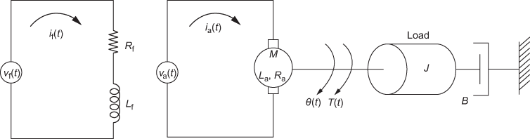
Fig. 13.8 ∣ Field-controlled DC motor

The parameters of DC machine are : is the field resistance in Ω, is the field inductance in H, is the field current in A, is the field voltage in V, is the back emf in V, is the torque developed by motor in N-m, is the angular displacement of shaft in rad, is the angular velocity of the shaft in rad/sec, is the moment of inertia of motor and load in kg-m²/rad and is the frictional ­coefficient of motor and load in N-m/(rad/sec).

An equivalent circuit of field is shown in Fig. 13.9.

Fig. 13.9 ∣ Electrical equivalent circuit of field

Applying Kirchhoff's voltage law to the circuit shown in Fig.13.9, we obtain

(13.18)

The torque output of DC motor is proportional to the product of flux and armature current. Since armature current is constant in the system (by keeping the armature voltage constant), the torque is proportional to flux, which is proportional to field current i.e., Therefore,

Torque, (13.19)

where is the torque constant in N-m/A.

A mechanical system of the DC motor is shown in Fig. 13.10.

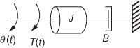
Fig. 13.10 ∣ Mechanical system of DC motor

The differential equation governing a rotational mechanical system of motor is given by

(13.20)

Substituting Eqn. (13.19) in Eqn. (13.20), we obtain

The state variables chosen are , and . The input variable is armature voltage, .

Substituting the state variables and input variable in Eqn. (13.18), we obtain

or

Simplifying, we obtain

(13.21)

Substituting the state variables in Eqn. (13.20), we obtain

Simplifying, we obtain

(13.22)

Also, (13.23)

Representing the Eqs. (13.21), (13.22) and (13.23) in matrix form, we obtain

(13.24)

The output variables are and .

Relating the output variables to state variables, we obtain

;

Representing the above equations in matrix form, we obtain

(13.25)

The state equation given by Eqn. (13.24) and the output equation given by Eqn. (13.25) together constitute the state-space model of the field-controlled DC motor shown in Fig. 13.11.

The block diagram representation obtained by combining the state variables given by Eqs. (13.21), (13.22) and (13.23) and the output variables is shown in Fig. 13.11.

Fig. 13.11 ∣ Block diagram representation of the state-space model field-controlled DC motor

13.9 State-Space Representation of a System Governed by Differential Equations

When a differential equation of a system is provided, the state equation and output equation are obtained by the selection of state variables and output variables which can be clearly understood with the following examples.

Solution: We choose the state variables as

, and .

Representing the given differential equation using the chosen state variables, we obtain

Therefore, the chosen state variables and above equation can be written in matrix form as

which is the state equation for the given system.

The output equation in matrix form is represented as

Solution: We chose the state variables as and

Representing the given differential equation using the chosen state variables, we obtain

Representing the chosen state variables and above equation in matrix form, we obtain

which is the state equation for the given system.

The output equation in matrix form is represented as

13.10 State-Space Representation of Transfer Function in Phase Variable Forms

The phase variables are the state variables which are obtained by assuming one of the system variables as a state variable and other state variables as the derivatives of the selected system variable. In most cases, the output variable which is one of the system variables is considered as the state variable. The state-space model of the system using phase variables can be obtained if and only if the differential equation of the system or the system transfer function is known. The state-space model of the system using phase variables can be obtained using three methods which are discussed below.

13.10.1 Method 1

Consider the order differential equation of a system as

(13.26)

where is the output and is the input.

Expressing the state variables in terms of the output , we obtain

(13.27)

and

Substituting all the equations of Eqn. (13.27) in Eqn. (13.26), we obtain

(13.28)

Simplifying Eqn. (13.28), we obtain

(13.29)

Representing Eqn. (13.27) and Eqn. (13.29) in matrix form, we obtain

(13.30)

Using Eqn. (13.27), we obtain the output equation as

(13.31)

Therefore, if the differential equation of a system is given by Eqn. (13.26), then the state-space model of such a system is given by

and

where , and .

If a matrix is of the form as given by matrix , then it is called the bush or companion form.

13.10.2 Method 2

Consider the order differential equation of a system as

(13.32)

To represent the system given by Eqn. (13.32) by state-space model, we consider

Therefore, Eqn. (13.32) will be simplified as

(13.33)

Taking Laplace transform and simplifying, we obtain

(13.34)

The SFG of Eqn. (13.34) is shown in Fig. 13.12.

Fig. 13.12

Let us consider the output of each integrator as the state variable. The number of state variables of the system is three as there are three integrators in the system as shown in Fig. 13.12.

Considering the state variables as , and , the SFG will be modified as shown in Fig. 13.13.

Fig. 13.13

From Fig. 13.13, we obtain

(13.35)

(13.36)

(13.37)

(13.38)

Representing Eqs. (13.35), (13.36) and (13.37) in matrix form, we obtain the state equation as

(13.39)

Representing Eqn. (13.38) in matrix form, we obtain the output equation as

(13.40)

Therefore, for an order system, the state equation and output equation are given by

13.10.3 Method 3

There exists another method to determine the state-space equations for the system represented by Eqn. (13.32).

To understand this method of state-space representation, we assume . ­Therefore, Eqn. (13.32) will be simplified as

(13.41)

Taking Laplace transform and simplifying, we obtain

(13.42)

Let

where (13.43)

and (13.44)

Simplifying Eqn. (13.43), we obtain

(13.45)

Taking inverse Laplace transform, we obtain

(13.46)

Let the state variables be

, and (13.47)

Substituting the above state variables in Eqn. (13.46), we obtain

or (13.48)

Simplifying Eqn. (13.44), we obtain

(13.49)

Taking inverse Laplace transform, we obtain

(13.50)

Substituting the state variables given by Eqn. (13.47) in the above equation, we obtain

(13.51)

Substituting Eqn. (13.48) in the above equation, we obtain

or (13.52)

Representing Eqs. (13.48) and (13.52) in matrix form, we get the state and output equations as

(13.53)

(13.54)

Therefore, for an order system, the state equation and output equation are given by

(13.55)

(13.56)

13.10.4 Advantages of Phase-Variable Representation

The advantages of phase-variable representation are:

1. The implementation is simple.
2. The state and output equations can be obtained by inspecting the differential ­equations constituting the system.
3. The transfer function design and time-domain design can be related easily by using the phase variables.
4. It is a powerful method for obtaining the mathematical model.
5. It is not necessary to consider the phase variables as the physical variables.

13.10.5 Disadvantages of the Phase-Variable Representation

The disadvantages of phase-variable representation are:

 

1. As the phase variables are not physical variables, the significance in measurement and control is lost for practical considerations.
2. It is difficult to obtain higher order derivatives of output.
3. It does not provide practical mathematical information.

Solution: Given

Taking inverse Laplace transform, we obtain

(1)

Let the chosen state variables be

(2)

and

Substituting Eqn. (2) in Eqn. (1), we obtain

(3)

Representing Eqs. (2) and (3) in matrix form, we obtain the state equation as

The output equation in matrix form is given by

Solution: The transfer function is converted to the form

The SFG of the above equation is shown in Fig. E13.8(a).

Fig. E13.8(a)

Let the output of each integrator be the state variable. The number of state variables of the system is three i.e., there are three integrators in the system as shown in Fig. 13.1(b). Considering the state variables as , and , the SFG will be modified as shown in Fig. E13.8(b).

Fig. E13.8(b)

From Fig. E13.8(b), the state equations are obtained as

Representing the above three equations in matrix form, we get the state equation as

The output equation in matrix form is given by

Solution: We know that

Let

where (1)

and (2)

Simplifying Eqn. (1), we obtain

Taking inverse Laplace transform, we obtain

(3)

Let the state variables for the system be

(4)

and

Substituting Eqn. (4) in Eqn. (3), we obtain

(5)

or (6)

Simplifying Eqn. (2), we obtain

Taking inverse Laplace transform, we obtain

(7)

Substituting Eqn. (4) in the above equation, we obtain

(8)

Substituting Eqn. (6) in Eqn. (8), we obtain

(9)

Representing Eqn. (4) and Eqn. (6) in matrix form, we get the state equations as

(10)

Representing Eqn. (9) in matrix form, the output equation is

13.11 State-Space Representation of Transfer Function in Canonical Forms

Consider a system defined by

where is the input and is the output.

Taking Laplace transform and simplifying, we obtain

13.11.1 Controllable Canonical Form

The transfer function for state-space representation in controllable canonical form is

(13.57)

The state and output equation for the above equation is obtained for (i) and (ii) .

Rewriting Eqn. (13.57), we obtain

(13.58)

where for

Therefore, the state equation is given by

The output equation is given by

Substituting in Eqn. (13.58), the transfer function is given by

Therefore, the state equation is given by

The output equation is given by

The controllable canonical form is important in discussing the pole-placement approach to the control systems design.

13.11.2 Observable Canonical Form

The transfer function for state-space representation in observable canonical form is

Therefore,

Rewriting the above equation, we obtain

where

with

Taking inverse Laplace transform and representing them in matrix form, the state ­equation is

(13.59)

The output equation is given by

(13.60)

Substituting in Eqn. (13.58), the transfer function is

Following similar procedure as done with , the state equation is given by

(13.61)

The output equation is

(13.62)

13.11.3 Diagonal Canonical Form

The transfer function for state-space representation in diagonal canonical form is

(13.63)

where , , … are residues and , , …, are roots of denominator polynomial (or poles of the system).

The Eqn. (13.63) can be rearranged as

(13.64)

(13.65)

Therefore,

(13.66)

The Eqn. (13.66) can be represented by block diagram as shown in Fig . 13.14.

Fig. 13.14

Assuming the output of each block as a state variable, we get the state equations as

(13.67)

The output equation is (13.68)

The state equation is given by

(13.69)

The output equation is given by

(13.70)

13.11.4 Jordan Canonical Form

Consider the case where the denominator polynomial involves multiple roots. Here, the preceding diagonal canonical form must be modified into the Jordan canonical form. Suppose, for example, that the roots of the denominator polynomial are different from one another, except for the first m roots then the transfer function for state-space ­representation in Jordan canonical form is

The partial-fraction expansion of the above equation becomes

To represent the above equation, let us assume that m = 3. Therefore,

Fig. 13.15

The state equations from the block diagram shown in Fig. 13.15 are

The output equation from the block diagram is

The state equation in matrix form is given by

(13.71)

The output equation is given by

(13.72)

Therefore, in general for number of equal roots, the state equation and the output equation in matrix form can be written as

The output equation is given by

Solution: Given

Comparing the above equation with the standard form as given in Eqn. (13.57), we find and the values for the controllable canonical form are

, , , and .

Using these values, the state-space model of the given system can be obtained as

Solution: Given

Comparing the above equation with the standard form as given in Eqn. (13.57), we find and the values for the observable canonical form are

, , , and .

Using these values, the state-space model of the given system can be obtained as

Solution: Given

Using partial-fraction expansion,

Here, (1)

Equating coefficients of on both sides, we obtain

(2)

Equating coefficients of constants on both sides of Eqn. (1), we obtain

(3)

Solving Eqs. (2) and (3), we obtain

and

Therefore,

Comparing the above equation with the standard diagonal canonical form, the coefficient values for the diagonal canonical form are

, , , and .

Using these values, the state-space model of the given system can be obtained as

and

Solution:

Given

Using partial-fraction expansion,

(1)

Equating coefficients of on both sides, we obtain

Equating coefficients of on both sides of the Eqn. (1), we obtain

(2)

Equating coefficients of constants on both sides of the Eqn. (1), we obtain

(3)

Solving Eqs. (1), (2) and (3), we obtain

, and

Comparing the above equation with the standard Jordan canonical form, the coefficient values for the diagonal canonical form are

, , , , and

Using these values, the state-space model of the given system can be obtained as

and

13.12 Transfer Function from State-Space Model

Let the state-space model of the system be

(13.73)

The Laplace transforms of the equations are

(13.74)

(13.75)

Rewriting Eqn. (13.74), we obtain

Therefore, (13.76)

where is an identity matrix.

Substituting Eqn. (13.76) in Eqn. (13.75), we obtain

Therefore, the transfer function

(13.77)

Here must have dimensionality and thus has elements. Therefore, for every input, there are transfer functions with one for each output which is the reason that the state-space representation can easily be the preferred choice for MIMO systems.

When the output and input are not directly connected, the matrix D will be a null matrix.

Therefore, the transfer function (13.78)

Solution: Since two columns exist in the B matrix, given system has two inputs , . Also, as two rows exist in the C matrix, given system has two outputs , . Therefore, four transfer functions exist for the given system which are given by

, , and

From the given state-space model, we obtain

Transfer function,

and

Hence, transfer function

Therefore, , , and

Solution: From the given model,

Transfer function is given by

Therefore, the transfer function is

Solution: The transfer matrix is given by

Therefore,

Transfer function,

Therefore,

13.13 Solution of State Equation for Continuous Time Systems

Consider a system with state equation as given by

(13.79)

The above state equation can be of homogenous or non-homogenous type.

13.13.1 Solution of Homogenous-Type State Equation

State equation is said to be of homogenous type when the system is free running (i.e., with zero input forces). Then the state equation becomes

(13.80)

The procedure for obtaining the solution for the above equation is discussed as follows.

Consider a differential equation as given by

(13.81)

The above equation is a homogeneous equation with zero input vector and with the initial condition .

The solution of Eqn. (13.81) is assumed to be given by

(13.82)

where are constants.

In the above equation, at .

Substituting Eqn. (13.82) in Eqn. (13.81), we obtain

Simplifying, we obtain

(13.83)

Equating the coefficients of constants and time, for in the above equation, we obtain

(13.84)

Therefore,

(13.85)

Substituting Eqn. (13.85) in Eqn. (13.82), we obtain

(13.86)

(13.87)

Substituting in the above equation, we obtain

(13.88)

In the above equation, represents an exponential series which is represented as .

Therefore, Eqn. (13.88) can be written as

The above equation is the solution of the homogenous equation in scalar form.

Therefore, for the state equation given by Eqn. (13.80), we have

The solution for the above equation is

(13.89)

where is not a scalar, but a matrix termed as State Transition Matrix (STM) of order , which will be discussed in the forthcoming sections.

13.13.2 Solution of Non-Homogenous Type State Equation

State equation is said to be of non-homogenous type when the system is with input forces. Then the state equation remains the same as given in Eqn. (13.79) which is given by

or (13.90)

Pre-multiplying both sides by we obtain

The above equation can be written as

(13.91)

Integrating Eqn. (13.91) with respect to time with limits and , we obtain

Therefore,

Pre-multiplying both sides by , we obtain

Therefore,

(13.92)

This is the solution for the state equation given by Eqn. (13.90).

From Eqn. (13.92), it is observed that the solution is divided into two different parts. The first part is the solution of homogenous-type state equation and it is termed as Zero Input Response (ZIR).

The second part is the solution due to the application of input from time 0 to . Therefore, the solution is termed as forced solution or Zero State Response (ZSR).

Thus, Eqn. (13.92) can be represented as

If the initial time is , then the solution is

13.13.3 State Transition Matrix

For obtaining the solution of the homogeneous and non-homogeneous state equations, it is necessary to determine the State Transition Matrix (STM).

The STM represented as will be defined and derived as follows:

For homogenous-type state equation,

Taking Laplace transform, we obtain

or

Therefore, (13.93)

Taking inverse Laplace transform, we obtain

(13.94)

Comparing the above equation with the solution of homogenous-type state equation, we obtain

Therefore,

where is called as the resolvent matrix, for which the inverse Laplace transform yields .

For non-homogenous-type state equation,

Taking Laplace transform, we obtain

or

Multiplying on both sides, we obtain

(13.95)

Taking inverse Laplace transform, we obtain

(13.96)

Comparing the above equation with the solution of non-homogenous-type state equation, we obtain

where is called as the resolvent matrix for which the inverse Laplace transform yields .

To prove that = :

We know that,

Therefore, (13.97)

Taking inverse Laplace transform, we get

(13.98)

Various procedures to determine the STM are discussed below:

Inverse Laplace Transform Method

We know that the resolvent matrix is given by

Taking inverse Laplace transform, we obtain

(13.99)

Series Summation method

We know that,

The series represented by the above equation is used to determine . The series summation method is better suited for digital computation. Assuming, and substituting in the above equation, we obtain

(13.100)

From the above equation, it is observed that each term in the above series contains the preceding term and a multiplier in a regular order. If the terms of the series are denoted as , then each term can be represented as

(13.101)

The series would converge quickly if exponential terms are present in it.

-matrix Method

By -matrix method, a non-singular matrix M, called the modal matrix is to be determined such that the transformation of state variable is given by

(13.102)

Differentiating, we obtain

(13.l02)

Therefore, substituting Eqs. (13.l01) and (13.l02) in state equation of a system, we obtain

(13.l03)

Multiplying Eqn. (13.l03) by on both sides, we obtain

(13.l04)

where

and (13.l05)

The transformation done in the above equations is called similarity transformation.

Proceeding further, it is required that eigen values and eigen vectors for a matrix are defined.

If is a matrix with order , is a non-zero vector and is a scalar such that

(13.l06)

Therefore, is the eigen vector and is an eigen value of , since eigen values and eigen vectors are interdependent (i.e., is the eigen vector corresponding to eigen value and is an eigen value corresponding to the eigen vector ).

By similarity transformation, matrix A is diagonalised with its diagonal elements being the eigen values.

That is, (13.l07)

The modal matrix can be obtained by the eigen vectors of as

where is the eigen vector corresponding to the eigen value .

Therefore, for the eigen vector , Eqn. (13.l06) becomes

(13.l08)

Representing the above equation in matrix form, we obtain

(13.l09)

Extending the above equation from eigenvector to eigenvector , we obtain

(13.l10)

or

(13.l11)

Equation (13.l11) can be represented as

(13.l12)

Multiplying the above equation by on both sides and rearranging the terms, we obtain

Therefore, (13.l13)

From the above equation, it is observed that by similarity transformation, modal matrix formed by the eigen vectors of diagonalises it.

However, if the matrix is of the phase-variable canonical form, the modal matrix may be given by

(13.l14)

where are the eigen values of .

By modal matrix, the STM is obtained from the similarity transformation of from Eqn. (13.l13) as

(13.l15)

From Eqn.(13.113), we have

(13.l16)

Therefore,

(13.l17)

13.13.4 Properties of State Transition Matrix

The properties of STM are

1. (13.118)
2. (13.119)

   Proof: Post multiplying both sides of Eqn. (13.98) by we obtain

   (13.120)

   Then, premultiplying both sides of Eqn. (13.98) by we obtain

   

   Therefore, (13.121)

   Thus, (13.122)

   An interesting result from this property, of Φ(t) is,

   (13.123)

   Which means that the state-transition process can be considered as bilateral in time, i.e., the transition in time can take place in either direction.

3. for any (13.124)

   Proof

   

   (13.125)

   This property of the STM is important since it implies that a state-transition process can be divided into a number of sequential transitions.

4.  for k-positive integer(13.126)

   Proof

   (13.127)

   

   The important properties of the STM are listed in Table 13.2.

   Table 13.2 ∣ Important properties of the STM

   

Solution: (a) To determine the STM

(i) Inverse Laplace Transform Method

Given

Therefore,

Taking inverse Laplace transform of the individual matrix elements,

Hence, (1)

(ii) Series Summation Method

Given

Therefore,

Also,

By series summation method,

Neglecting higher order terms, considering till n = 3 and substituting, and in the above equation, we obtain

(2)

(b) Solution of the System

As the system is given by , the solution of the system has two parts as given by

(3)

Substituting , , and STM in Eqn. (3), we obtain

Therefore, the solution with State Vectors and are

and

Solution: To determine STM :

Given

Therefore,

Solving the equation the eigen values of matrix are and

If is the eigen vector corresponding to the eigen value , then the equation must be satisfied.

Since ,

the equations obtained from the above matrix are

(1)

(2)

Solving Eqs. (1) and (2), we obtain

Assuming , the eigen vector associated with the eigen value is

If is the eigen vector corresponding to the eigen value , then the equation must be satisfied.

i.e.,

The equations obtained from the above matrix are

Solving Eqs. (3) and (4), we obtain .

Assuming and , the eigen vector associated with the eigen value is

Therefore, the modal matrix is

Taking inverse for the above matrix, we obtain

It is noted that if modal matrix is correctly formed, it should diagonalise through similarity transformation with the diagonal elements remaining the same as the determined eigen values. It is observed that,

(3)

The above matrix shows that the determined modal matrix is correct since diagonal elements are same as the determined eigen values.

Since ,

Therefore, STM,

(4)

Solution of the System

As the system is of homogenous type (i.e., ), solution of the system is given by

(5)

Substituting , and STM in Eqn. (5), we obtain

Therefore, the solutions with state vectors and are

and

13.14 Controllability and Observability

A system is said to be controllable, if there exists some finite control vector that will bring the system from any initial state at to any specific desired state in the state-space, within a specified finite time interval given by .

Observability is the dual of controllability, by which it is possible to construct an input vector , which is unconstrained, transferring an initial output to a final output within a specified finite time interval . Thus, the system is said to be observable if the outputs can be measured by identifying every state within a specified finite time interval.

13.14.1 Criteria for Controllability

A system with state equation, and output equation, is said to be controllable if the controllability matrix of order given by

has rank .

13.14.2 Criteria for Observability

A system with state equation, and output equation, is said to be observable, if the observability matrix of order given by

has rank .

Solution: Comparing the standard state-space model of the system with the given state-space model, we obtain

Controllable

To check whether the system is controllable or not, the controllability matrix is to be determined using the state-space model of the system.

Since the order of matrix is 3, the controllability matrix is given by

The controllability matrix for the given state-space model of the system is formed as ­follows:

Step 1:

Step 2:

Step 3:

Step 4: Therefore,

Step 5: Since is not a square matrix, it is necessary to check all the possibility of higher order square matrix that can be obtained from . In this case, the higher order matrix that can be obtained from is . The number of matrix that can be obtained from is 20. Therefore, if the determinant value of any one of 20 matrices is non-zero, then the system is said to be completely controllable. For the obtained , the determinant value of all the matrix is non-zero, therefore the rank of .

Step 6: Since the rank of controllability matrix and order of matrix are same, the given system is completely controllable.

Observable

To check whether the system is observable or not, the observability matrix is to be determined using the state-space model of the system.

Since the order of matrix is 3, the observability matrix is given by

The observability matrix for the given state-space model of the system is formed as:

Step 1:

Step 2:

Step 3:

Step 4: Therefore,

Step 5: . Therefore, rank of .

Step 6: Since the rank of observability matrix and order of matrix are same, the given system is completely observable.

Therefore, the given system is completely controllable and observable.

Fig. E13.21(a)

Solution: The state equations are obtained by considering the blocks shown in Fig. 13.21(a).

Consider the first block as shown in Fig. E13.21(b).

Fig. E13.21(b)

From Fig. 13.21(b), it is observed that

Therefore,

Taking inverse Laplace transform, we obtain

(1)

Consider the second block as shown in Fig. E13.21(c).

Fig. E13.21(c)

From Fig. 13.21(c), it is observed that

Taking inverse Laplace transform, we obtain

(2)

Consider the third block as shown in Fig . E13.21(d).

Fig. E13.21(d)

From Fig. E13.21(d), it is observed that

Simplifying, we obtain

Taking inverse Laplace transform, we obtain

(3)

Differentiating Eqn. (2) with respect to , we obtain

Substituting the above equation and Eqn. (2) in Eqn. (1) and simplifying, we obtain

(4)

Let the output (5)

Using Eqs. (2), (3) , (4) and Eqn. (5), the required state-space model of the system is given by

(state equation)(6)

(output equation)(7)

From Eqs. (6) and (7), we obtain

, and

Controllable

To check whether the system is controllable or not, the controllability matrix is to be determined using the state-space model of the system.

Since the order of matrix is 3, the controllability matrix is given by

The controllability matrix for the given state-space model of the system is formed as g:

Step 1:

Step 2: =

Step 3:

Step 4: Therefore,

Step 5: . Therefore, rank of .

Step 6: Since the rank of controllability matrix and order of matrix are same, the given system is completely controllable.

Observable

To check whether the system is observable or not, the observability matrix is to be determined using the state-space model of the system.

Since the order of matrix A is 3, the observability matrix is given by

The observability matrix for the given state-space model of the system is formed as follows:

Step 1:

Step 2:

Step 3:

Step 4: Therefore,

Step 5: . Therefore, rank of .

Step 6: Since the rank of observability matrix and order of matrix are same, the given system is completely observable.

Therefore, the given system is completely controllable and observable.

13.15 State-Space Representation of Discrete-Time LTI Systems

Consider a SISO discrete-time LTI system which is described by an Nth-order difference equation

(13.128)

Here, if is given for Eqn. (13.128) requires N initial conditions to uniquely determine the complete solution for n > 0. Thus, N values are required to specify the state of the system at any time.

Then, N state variables are defined as

(13.129)

Then from Eqs. (13.128) and (13.129), we have

and

In matrix form, the above equations can be expressed as

(13.130)

(13.131)

Equations (13.130) and (13.131) can be rewritten compactly as

(13.132)

(13.133)

where ; and is the matrix (or N-dimensional vector) state vector which is given by

Equations (13.132) and (13.133) which represent the state equation and output equation are called as N-dimensional state-space representation of the system and the matrix A is called the system matrix.

If a discrete-time LTI system has m inputs and p outputs and N state variables, then a state-space representation of the system can be represented as

where , and

and matrices ,

and

where is a matrix of order , is a matrix of order , is a matrix of order , is a matrix of order , is a matrix of order , is a matrix of order and is a matrix of order .

13.15.1 Block Diagram and SFG of Discrete State-Space Model

The basic block which is to be used in representing the discrete state-space model using block diagram technique is the delay unit (in continuous state-space model it is integrator block). The steps to be followed in representing the discrete state-space model using block diagram is similar to the steps discussed in Section 13.3. The block diagram representation of the discrete state-space model is shown in Fig. 13.16.

Fig. 13.16 ∣ Block diagram of the state-variable model

The SFG representation for the block diagram of the system shown in Fig. 13.16 is shown in Fig. 13.17.

Fig. 13.17 ∣ SFG representation of the state-variable model

13.16 Solutions of State Equations for Discrete-Time LTI Systems

Consider an N-dimensional state representation

(13.134)

(13.135)

where A, B, C and D are and matrices, respectively.

Taking the z-transform of Eqs. (13.134) and (13.135) and using time-shifting property of z-transform, we obtain

(13.136)

(13.137)

where and

where

Rearranging Eqn. (13.136), we have

(13.138)

Premultiplying both sides by , we obtain

(13.139)

Taking inverse z-transform, we obtain

(13.140)

Substituting Eqn. (13.140) in Eqn. (13.135), we obtain

(13.141)

13.16.1 System Function H(z)

The system function H(z) of a discrete-time LTI system is defined by with zero initial conditions. Thus, setting = 0 in Eqn. (13.140), we have

(13.142)

Substituting Eqn. (13.142) in Eqn. (13.137), we obtain

Thus,

13.17 Representation of Discrete LTI System

The methods used for representing continuous linear time-invariant systems which have been discussed in Sections 13.10 and 13.11 are also applicable to the discrete linear time-invariant systems except for the fact that is replaced by .

Solution: Comparing the given system function with Eqn. (13.34), we can get the state and output equations as

Solution: Given

Therefore,

Therefore,

and

Solution: The given equation can be expressed as

Therefore, the block diagram representation for the above equations is shown in Fig. E13.23.

Fig. E13.23

13.18 Sampling

Let be a continuous-time varying signal. The signal which is shown in Fig . 13.18(a) is sampled at regular intervals of time with sampling period T as shown in Fig. 13.18(b). The sample signal is given by

(13.143)

Fig. 13.18 ∣ (a) Continuous-time signal and (b) sampling of a continuous-time signal

A sampling process can be interpreted as a modulation or multiplication process, as shown in Fig. 13.19.

Fig. 13.19 ∣ Periodic sampling of

The continuous-time signal is multiplied by the sampling function which is a series of impulses (periodic impulse train); the resultant signal is a discrete-time signal .

(13.144)

13.18.1 Sampling Theorem

The sampling theorem states that a band-limited signal having finite energy which has no frequency components higher than Hz can be completely reconstructed from its samples taken at the rate of samples per second (i.e., where is the sampling frequency and is the highest signal frequency.

The sampling rate of samples per second is the Nyquist rate and its reciprocal is the Nyquist period. For simplicity, is denoted as .

13.18.2 High Speed Sample-and-Hold Circuit

Figure 13.20(a) shows a sample-and-hold circuit for high speed of operation. The MOS transistor M shown is an analog switch is capable of switching by logic levels, such as that from TTL. It alternately connects and disconnects the capacitor to the output of op-amp . Diodes and are inverse-parallel connected. They prevent op-amp from getting into saturation when the transistor M is OFF. This makes the operation of the circuit faster. Hence, the output of op-amp will be when and when .

When transistor M is ON, the op-amps and act as voltage followers. The waveforms shown in Fig . 13.20(b) illustrate the operation of the circuit. The transistor is alternately switched ON and OFF by the control voltage at its gate terminal. Note that the voltage must be higher than the threshold voltage of the FET. When the transistor switch is ON for a short interval of time, the capacitor quickly charges or discharges to the value of the analog signal at that instant. In other words, when input is larger than capacitor voltage and the transistor is OFF, it rapidly charges to the level of the instant M switches ON. Similarly, if is initially greater than , then rapidly discharges to the level of when becomes ON.

When M is OFF, only the input bias current of op-amp and the gate-source reverse leakage current of FET are effective in discharging the capacitor. Hence, the sampled voltage is held constant by until the next sampling instant or acquisition time. Figure 13.20(c) shows the sampling or acquisition time and holding time . During the sampling time , is charged through the FET channel resistance and the charging time when the capacitor charges to 0.993 of input voltage. During the hold time , the capacitor partially discharges. This is called hold-mode droop. To avoid this, the op-amp must have very low input bias current, the capacitor should have a low leakage dielectric and M must have very low reverse leakage current between its gate and source terminals. The low ­channel resistance is desirable for the FET to achieve faster charging and ­discharging of .

Fig. 13.20(a) ∣ Sample-and-hold circuit

Fig. 13.20(b) ∣ Signal voltage, control voltage and output voltage waveforms

Fig. 13.20(c) ∣ Capacitor voltage waveform

13.18.2.1 Continuous-Data Control Systems

In continuous-data control system, the signals at various parts of the system are l functions of the continuous-time variable t. Examples for continuous-data control system include AC control system and DC control system.

In DC control system, the signals are unmodulated. The schematic diagram of a closed-loop DC control system with waveforms of the signals in response to a step-function input are also shown in Fig. 13.21. Typical components of a DC control system are DC tachometers, potentiometers, DC motors, etc.

Fig. 13.21 ∣ Schematic diagram of a typical DC closed-loop control system

In AC control system, the signals are modulated. The schematic diagram of a typical AC control system is shown in Fig. 13.22. The modulated information signal transmitted by an AC carrier signal is demodulated by the low-pass characteristics of the AC motor. AC control systems are used extensively in aircraft and missile control systems, wherein noise and disturbance often cause problems. By using modulated AC control systems with carrier frequencies of 400 Hz or higher, the system will be less vulnerable to low-frequency noise. Typical components of an AC control system are synchros, AC amplifiers, gyroscopes, accelerometers, AC motors, etc.

Fig. 13.22 ∣ Schematic diagram of a typical AC closed-loop control system

13.18.2.2 Discrete-Data Control Systems

In discrete-date control systems, the signals provided to the system are in the form of either train of pulses or a digital code. Discrete-data control systems are divided into sampled-data and digital control systems. In sampled-data control systems the signals are in the form of pulse data. In digital-data control system digital computer or controller is used in the system so that the signals are digitally coded.

In general, a sampled-data system receives data or information intermittently at specific instants of time. For example, the error signal in the sampled-data control system can be supplied only in the form of pulses, which has information about the error signal during the periods between two consecutive pulses.

Figure 13.23 shows the block diagram of sampled-data control system. A continuous-data input signal , applied to the system is compared with the output signal and the error signal is sent to the sampler, from which a sequence of pulses are obtained as output. The sampling rate of the sampler can be uniform or non-uniform. The advantages of the sampling operation is that expensive equipment used in the system may be utilized effectively as it would be time-shared among several other control equipments and noise cancellation is effectively achieved.

Fig. 13.23 ∣ Block diagram of sampled-data control system

Digital computers provide many advantages such as reduced size and increased flexibility. Hence, computer control is a popular technique employed in recent times. Figure 13.24 shows the block diagram of a digital-data control system which is used as autopilot for guided missile control.

Fig. 13.24 ∣ Example for digital-data control system (a guided missile)

Review Questions

1. Explain the concept of state.
2. Define a) state variables b) state vector and c) state-space.
3. What are the advantages of state-space analysis?
4. What do you mean by homogenous and non-homogenous state equations?
5. Define state transition matrix.
6. What are the properties of state transition matrix?
7. What are the advantages and disadvantages of representing the system using phase ­variables?
8. What are the advantages and disadvantages of representing the system using canonical variables?
9. What are the different methods available in representing the system using state-space model?
10. Define controllability and observability.
11. What is the difference between continuous-time signal and discrete-time signal?
12. What is a sampler?
13. Explain the sampling process.
14. Check the following systems for controllability and observability:
    1. , ,
    2. , ,
    3. , ,
15. The state equation for a system is . Determine the unit step response of the system when .
16. The state equation for a homogenous system is . Determine the solution of the system when .
17. Determine the system matrix for a certain system when , we have and when , we have .
18. The state-space model of a system is given by and . Determine the transfer function of the system.
19. The state-space model of a system is given by and . Determine the transfer function of the system.
20. Obtain the state-space model of the system whose transfer function is given by in Jordan cananonical form.
21. The transfer function of the system is given by . Determine the state-space model of the system using phase variables.
22. The differential equation of a system is given by Determine the state-space model of the system.
23. Determine the STM for a system whose matrix is given by .
24. The difference equation of a system is given by Determine the state-space model of the system.