9.1 Introduction to Polar Plot

The presence of magnitude plot and phase plot for showing the variation of gain and phase angle of a system with respect to the change in frequency is the major disadvantage of the Bode plot. The plot that combines both the plots to a single plot without losing any information is called polar plot. The polar plot can be plotted either on a polar graph or on an ordinary graph. Hence, polar plot for a particular system can be defined in two ways based on the graph used for plotting. The two different definitions for polar plot are given below:

The polar plot of a loop transfer function is defined as a plot of versus on the polar coordinates as the frequency varies from zero to infinity when it is plotted on a polar graph. Also, it is defined as a plot of real part of versus imaginary part of as the frequency varies from zero to infinity when it is plotted on an ordinary graph. The real and imaginary parts of the transfer function can be denoted as and respectively.

The concentric circles present in the polar graph represent the magnitude of the transfer function and the radial lines crossing the circles represent the phase angle of the transfer function. The phase angle of the transfer function can either be positive or negative. Hence, it can be noted that on a polar graph, positive phase angle is measured in counterclockwise direction and negative phase angle is measured in clockwise direction. A simple example of polar plot of a transfer function on an ordinary graph and on a polar graph is shown in Figs. 9.1(a) and (b) respectively.

Fig. 9.1 ∣ Polar plot on a graph

9.2 Starting and Ending of Polar Plot

The polar plot of any system starts from one quadrant on an ordinary graph and ends at the other quadrant. The starting and ending point of the polar plot depends on the type and order of the loop transfer function.

The starting point of the polar plot depends on the type of the loop transfer function of a given system as shown in Fig. 9.2(a). If the type of the loop transfer function of a given system is greater than 3, then the starting point of such system follows the system with type .

Fig. 9.2 ∣ Starting and ending points of polar plot

The ending point of the polar plot depends on the order of the loop transfer function as shown in Fig. 9.2(b). Similar to the starting point of the polar plot, if the order of the loop transfer function of the given system m > 4, then the ending point of such system follows the system with order .

It can be noted that this method of determining the starting and ending points of the polar plot is applicable to the system whose loop transfer function has only poles. In addition, it is applicable only if the plot is plotted on an ordinary graph sheet.

9.3 Construction of Polar Plot

The construction of polar plot can be illustrated by considering the generalized form of loop transfer function as

where are real constants,

is the number of zeros at the origin,

is the number of poles at the origin or the type of the system,

is the number of simple poles existing in the system,

is the number of simple zeros existing in the system,

is the number of complex poles existing in the system,

is the number of complex zeros existing in the system and

is the time delay in seconds.

Substituting in the above equation and simplifying, we obtain

(9.1)

Its magnitude is

(9.2)

and the phase angle is

(9.3)

where the magnitude of the term is 1 and phase angle of the term is .

From Eqn. (9.1), it is clear that the open-loop transfer function may contain the combination of any of the following five factors:

1. Constant K
2. Zeros at the origin and poles at the origin
3. Simple zero and simple pole
4. Complex zero and complex pole
5. Transportation lag

Hence, it is necessary to have a complete study of magnitude and phase angle of these factors that can be utilized in constructing the polar plot of a composite loop transfer function . The polar plot for the loop transfer function is constructed by determining its magnitude and phase angle. The magnitude and phase angle of the loop transfer function can be obtained by the multiplication of magnitudes and addition of the phase angles of individual factors present in the function.

Also, if the polar plot of is to be plotted on an ordinary graph, the magnitude and phase angle of obtained at different frequencies are converted to the real and imaginary parts of . Hence, it becomes necessary to determine the magnitude and phase angle of each factor which can be possibly present in a system.

Factor 1: Constant

The constant is independent of frequency and hence the magnitude and phase angle of the factor are:

Magnitude :

Phase angle :

In addition, the real and imaginary parts of constant K are K and 0 respectively.

Since the magnitude, real part and imaginary part of constant K are independent of frequency, the polar plot of constant is a point on both polar graph and ordinary graph. The polar plot for constant on polar graph and on an ordinary graph is shown in Figs. 9.3(a) and (b) respectively.

Fig. 9.3 ∣ Polar plot for constant K

Factor 2: Zeros at the origin and poles at the origin

The zeros at the origin and poles at the origin are dependent on frequency . Hence, the magnitude and phase angle when one pole or zero exists at the origin are given in Table 9.1(a).

Since the magnitude and phase angle of the factors are dependent on frequency , the polar plot for the factor on polar graph can be drawn with the help of Table 9.1(a).

Table 9.1(a) ∣ Magnitude and Phase angle for jω and (jω)⁻¹ for different values of frequency ω

The polar plot for and on polar graph is shown in Figs. 9.4(a) and (b) respectively.

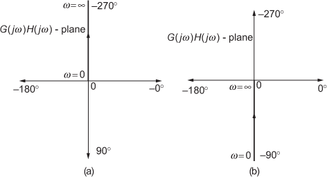
Fig. 9.4 ∣ Polar plot for and on polar graph

When more than one pole or zero exist at the origin, the changes to be done in plotting the polar plot on polar graph is given in Table 9.1(b).

Table 9.1(b) ∣ Magnitude and phase angle of and

When more than one pole or zero exist at the origin, the changes to be done in plotting the polar plot on an ordinary graph are not as easy as they are on polar graph. The reason is that depending on and , the real and imaginary parts vary. For example, if the real part is zero, whereas if the imaginary part is zero.

Therefore, the polar plot for different values of and rotates by either in the clockwise direction or in the anticlockwise direction on an ordinary graph. The polar plots of for different values of on an ordinary graph are shown in Figs. 9.4(c) through (f).

Similarly, the polar plot of ( jω)^-N for different values of N can be drawn on an ordinary graph. In addition, the polar plots of ( jω)^Z and ( jω)^-N for different values of Z and N can be drawn on polar graph.

Fig. 9.4 ∣ Polar plot for different values of

It can be noted that if the polar plot of is drawn on an ordinary graph and it is rotated by in the clockwise or anticlockwise direction, the polar plot of can be obtained, provided .

Factor 3: Simple zero (1 + jωT) and simple pole (1 + jωT)⁻¹

The simple zero and simple pole are dependent on frequency . Hence, the magnitude and phase angle of simple zero and simple pole are given in Table 9.2.

Since the magnitude and phase angle are dependent on frequency , the polar plot for a simple zero and simple pole on polar graph can be drawn using Table 9.2.

Table 9.2 ∣ Magnitude and Phase angle for and for different values of frequency ω

The polar plots for and on the polar graph are shown in Figs. 9.5(a) and (b) respectively.

Fig. 9.5 ∣ Polar plot for and on polar graph

Factor 4: Complex zero (1 + j2ξu_n − u_n²) and complex pole (1 + j2ξu_n − u_n²)⁻¹

The complex zero and complex pole are dependent on frequency . Hence, the magnitude and phase angle of the factors are given in Table 9.3(a).

Table 9.3(a) ∣ Magnitude and phase angle of and

In Table 9.3(a), is the damping ratio and .

Since the magnitude and phase angle of the factors are dependent on frequency , the polar plot for the factor on the polar graph can be drawn using Table 9.3(b).

Table 9.3(b) ∣ Magnitude and Phase angle for and for different values of frequency ω

The polar plots for and on the polar graphs for different values of are shown in Figs. 9.6(a) and (b) respectively.

Fig. 9.6 ∣ Polar plots for and on the polar graph

Factor 5: Transportation lag

The factor can be rewritten as . The magnitude and phase angle of the factor are

Magnitude of

and Phase angle =

But the phase angle obtained is in the unit of radians. Therefore, the phase angle in degrees is obtained as

Fig. 9.7 ∣ Polar plot of transportation lag

Since the magnitude of the factor is independent of frequency , the polar plot for the factor on polar graph and on an ordinary graph is a unit circle, which are shown in Figs. 9.7(a) and (b) respectively.

9.4 Determination of Frequency Domain Specification from Polar Plot

The different frequency domain specifications such as gain margin, phase margin, phase crossover frequency and gain crossover frequency can be determined by using polar plot. As the polar plots can be plotted both on polar graph and ordinary graph, the determination of frequency domain specification also differs.

9.4.1 Gain Crossover Frequency ω_gc

It is the frequency at which the magnitude of the loop transfer function is unity. This frequency can be obtained by substituting random frequencies in Eqn. (9.2). But by this process, we can obtain only an approximate value of frequency and also this process is time-consuming. Hence, there exist two alternate methods for determining which are discussed below:

Method 1: It is known that = 1 at . Also, Eqn. (9.2) is a function of frequency. Therefore, by solving the equation, we obtain . This method consumes more time.

Method 2: From the polar plot drawn on the polar graph, it is easy to determine the when . Substituting the obtained angle in Eqn. (9.3) and using , it is easy to determine .

Hence, method 2 is used in this chapter for determining the gain crossover frequency when a polar plot for a loop transfer function is drawn.

9.4.2 Phase Crossover Frequency ω_pc

It is the frequency at which the phase angle of the loop transfer function is or . This frequency can be obtained by substituting random frequencies in Eqn. (9.3). But by this process, we can obtain only an approximate value of frequency and also this process is a time-consuming one. Hence, an alternate method exists for determining as discussed below:

Alternate method

It is known that at . Hence, using , the value of can be determined.

9.4.3 Gain Margin g_m

The gain margin of the system obtained by taking the inverse of the magnitude of at phase crossover frequency .

9.4.4 Phase Margin p_m

The phase margin of the system is obtained by

9.5 Procedure for Constructing Polar Plot

The flow chart for constructing the polar plot of a system on a polar graph is shown in Fig. 9.8(a).

Fig. 9.8(a) ∣ Flow chart for constructing the polar plot on polar graph

The flowchart for constructing the polar plot of a system on an ordinary graph is shown in Fig. 9.8(b).

Fig. 9.8(b) ∣ Flow chart for constructing the polar plot on an ordinary graph

Intersection of polar plot for a system

If the polar plot intersects line on a polar graph, it implies that the polar plot intersects the positive real axis line on an ordinary graph. Therefore, there exists a relation between the intersection points on an ordinary graph and on a polar graph which is listed in Table 9.4.

Table 9.4 ∣ Relation between intersection points

In addition, it is to be noted that if number of intersection points exists in plotting the polar plot on a polar graph, same number of intersection points exists in plotting the polar plot on an ordinary graph.

9.6 Typical Sketches of Polar Plot on an Ordinary Graph and Polar Graph

The typical sketches of polar plot on an ordinary and polar graph based on the type and order of a system are given below.

Type 0 Order 2 System

Let the loop transfer function of Type 0 Order 2 system be

Substituting , we obtain

The magnitude and phase angle of the system are given by

and

The magnitude and phase angle at and are given in Table 9.5.

Table 9.5 ∣ Magnitude and phase angle of the system

To determine the intersection point on real and imaginary axis

The real and imaginary part of loop transfer function can be determined as

Therefore, real part of loop transfer function

and imaginary part of loop transfer function

Intersection point on imaginary axis

Step 1: Equating the real part of loop transfer function to zero and determining the frequency i.e., .

Therefore,

Upon solving, we obtain

Step 2: Substituting in the imaginary part of loop transfer function, we obtain the intersection of the polar plot on imaginary axis.

Intersection point on imaginary axis =

Substituting in , we obtain

Step 3: Therefore, magnitude and phase angle of loop transfer function at is

Magnitude

and Phase angle

Using the magnitude and phase angle at different frequencies, we can determine the real and imaginary parts of the loop transfer function as given in Table 9.6.

Table 9.6 ∣ Real and imaginary parts of the system

Using Table 9.6, the polar plot of TYPE 0 ORDER 2 system on an ordinary graph is shown in Fig. 9.9(a).

Fig. 9.9(a) ∣ Polar plot of the system

The magnitude and phase angle at different frequencies are given in Table 9.7.

Table 9.7 ∣ Magnitude and phase angle

Using Table 9.7, the polar plot of TYPE 0 ORDER 2 system on polar graph is shown in Fig. 9.9(b).

Fig. 9.9(b) ∣ Polar plot of the system

Similarly, the polar plot on a polar graph and intersection points on the different axes for different systems can be determined.

9.7 Stability Analysis using Polar Plot

The stability of a system can be examined from the polar plot once the frequency domain specifications are obtained. The stability of the system can be analyzed by using the crossover frequencies ( and ) or the gain and phase margins.

9.7.1 Based on Crossover Frequencies

A system can either be a stable system or marginally stable system or unstable system. The stability of the system based on the relation between crossover frequencies is given in Table 9.8.

Table 9.8 ∣ Stability of the system based on crossover frequencies

9.7.2 Based on Gain Margin and Phase Margin

The stability of a system based on the gain margin and phase margin is given in Table 9.9.

Table 9.9 ∣ Stability of the system based on and

But the problem that exists in examining the stability of the system from polar plot is the determination of and which is a tedious process. Hence, an alternate way of examining the stability of the system using polar plot exists, which does not require the determination of and is discussed in the following section.

9.7.3 Based on the Location of Phase Crossover Point

Consider the polar plot of a loop transfer function drawn on an ordinary graph as shown in Fig. 9.10.

Let and be the points on the polar plot when the plot crosses the real axis and unit circle as shown in Fig. 9.10. Using Table 9.5, the points and are called phase crossover and gain crossover points respectively. Let the frequency at the point is the phase crossover frequency and magnitude of the loop transfer function at the point be

Fig. 9.10 ∣ Polar plot of a loop transfer function in an ordinary graph

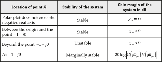
Now, based on the location of point , the stability of the system can be examined. The stability of the system based on the location of point is listed in Table 9.10.

Table 9.10 ∣ Stability of the system based on phase crossover point,

9.8 Determining the Gain K from the Desired Frequency Domain Specifications

The frequency domain specifications for which the gain can be determined are gain margin and phase margin. The procedure for determining the gain for the desired and using polar plot is not so tedious as it was using Bode plot. The following sections describe how the gain can be determined for desired and using polar plot.

9.8.1 When the Desired Gain Margin of the System is Specified

The step-by-step procedure to determine the gain for a specified gain margin is explained below:

Step 1: Assume for the given loop transfer function and construct the polar plot of the system either on the polar graph or on the ordinary graph.

Step 2: Determine the phase crossover point, from the polar plot. If the polar plot is plotted on the polar graph, the point refers to the point at which the polar plot crosses line and if the polar plot is plotted on the ordinary graph, the point refers to the point at which the polar plot crosses negative real axis.

Step 3: Determine the magnitude of the loop transfer function at from the polar plot. Let it be .

Step 4: Let the desired gain margin of the system be dB. Let be the phase crossover point on the polar plot corresponding to . The magnitude of the loop transfer function at can be determined by using

Step 5: Now, the gain for the desired gain margin can be determined as

Step 6: With the gain , the new polar plot can be drawn. The polar plot for different values of is shown in Fig. 9.11(a).

Fig. 9.11(a) ∣ Polar plot for different values of

9.8.2 When the Desired Phase Margin of the System is Specified

The step-by-step procedure to determine the gain for a specified phase margin is explained below:

Step 1: Assume for the given loop transfer function and construct the polar plot of the system either on the polar graph or on the ordinary graph.

Step 2: Determine the gain crossover point, from the polar plot. If the polar plot is plotted on the polar graph or on the ordinary graph, the point refers to the point at which the polar plot crosses unity circle.

Step 3: Determine the magnitude of the loop transfer function at from the polar plot. Let it be .

Step 4: Let the desired phase margin of the system be dB. Let be the gain crossover point on the polar plot corresponding to .

Step 5: Determine the phase angle of the system corresponding to . Let it be deg. The value of is determined by using, .

Step 6: Draw a radial line using deg from origin that cuts the polar plot of the loop transfer function with at . The magnitude of the loop transfer function at can be determined from the polar plot and let it be .

Step 7: Now, the gain for the desired gain margin can be determined as

Step 8: With the gain , the new polar plot can be drawn. The polar plot for different values of is shown in Fig. 9.11(b).

Fig. 9.11(b) ∣ Polar plot for different values of

Solution:

1. The loop transfer function of the system .
   

   Fig. E9.1

2. Substituting in the loop transfer function, we obtain

   

3. The only one corner frequency existing in the system is rad/sec.
4. The magnitude and phase angle of the system are

   and

5. For different values of frequency , the magnitude and phase angle of the system are calculated and tabulated in Table E9.1.

Table E9.1 ∣ Magnitude and phase angle of the system

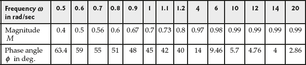
The polar plot of the given system using Table E9.1 is shown in Fig. E9.1.

Solution:

1. The loop transfer function of the system .
2. Substituting and in the loop transfer function, we obtain

   

3. The three corner frequencies existing in the system are

   rad/sec, rad/sec and rad/sec

   

   Fig. E9.2 ∣ Polar plot for

4. The magnitude and phase angle of the system are

   

   and

5. For different values of frequency , the magnitude and phase angle of the system are calculated and tabulated in Table E9.2.

Table E9.2 ∣ Magnitude and phase angle of the system

The polar plot of the given system using Table E9.2 is shown in Fig. E9.2.

Solution:

1. The loop transfer function of a system is .
2. Substituting , we obtain

   

3. The three corner frequencies existing in the system are rad/sec, rad/sec and rad/sec.
4. The magnitude and phase angle of the system are

   

   and

   

   Fig. E9.3 ∣ Polar plot for

5. For different values of frequency , the magnitude and phase angle of the system are calculated and tabulated in Table E9.3.

Table E9.3 ∣ Magnitude and phase angle of the system

The polar plot of the given system using the data in Table E9.3 is shown in Fig. E9.3.

Solution:

1. The loop transfer function of a system is .
2. Substituting , we obtain

   

3. The corner frequency of the given system is rad/sec.
4. The magnitude and phase angle of the system are

   

   and

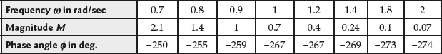
5. For different values of frequency , the magnitude and phase angle of the system are calculated and tabulated in Table E9.4.

Table E9.4 ∣ Magnitude and phase angle of the system

The polar plot of the given system using Table E9.4 is shown in Fig. E9.4.

Fig. E9.4

Determination of Gain Margin and Phase Margin

The gain margin and phase margin of the system are calculated at phase crossover frequency and gain crossover frequency respectively. The phase crossover frequency is the frequency at which the phase angle of the system is or . Also, the gain crossover frequency is the frequency at which the magnitude of the system is 1.

Using the above definition and Table E9.4, we obtain

Gain crossover frequency rad/sec and Phase crossover frequency rad/sec.

Hence, gain margin and phase margin of the system are given by

Gain margin,

and Phase margin,

Solution:

1. The loop transfer function of a system is
2. Substituting , we obtain

   

3. The two corner frequencies existing in the given system are

   rad/sec and rad/sec respectively.

4. The magnitude and phase angle of the system are

   

   and

   

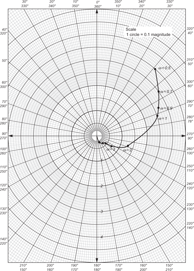
   Fig. E9.5

5. For different values of frequency , the magnitude and phase angle of the system are calculated and tabulated in Table E9.5.

Table E9.5 ∣ Magnitude and phase angle of the system

The polar plot of the given system using the data in Table E9.5 is shown in Fig. E9.5.

9.9 Introduction to Nyquist Stability Criterion

The Routh–Hurwitz criterion and root locus methods are used to determine the stability of the linear single-input single-output (SISO) system by finding the location of the roots of the characteristic equation in s-plane. The Nyquist stability criterion derived by H. Nyquist is a semi-graphical method that helps in determining the absolute stability of the closed-loop system graphically from frequency response of loop transfer function (Nyquist plot) without determining the closed-loop poles. The Nyquist plot of a loop transfer function is a graphical representation of the frequency response analysis when the frequency is varied from to . Since most of the linear control systems are analyzed by using their frequency responses, Nyquist plot will be convenient in determining the stability of the system.

9.10 Advantages of Nyquist Plot

The advantages of Nyquist plot are:

1. Nyquist plot helps in determining the relative stability of the system in addition to the absolute stability of the system.
2. It determines the stability of the closed-loop system from open-loop transfer function without calculating the roots of characteristic equation.
3. It gives the degree of instability of an unstable system and indicates the ways in which the stability of the system can be improved.
4. It gives information related to frequency domain characteristics such as , BW etc..
5. It can easily be applied to systems with pure time delay that cannot be analyzed using root locus method or Routh–Hurwitz criterion.

9.11 Basic Requirements for Nyquist Stability Criterion

The Nyquist stability criterion will be useful in analyzing the stability of both the open-loop and closed-loop systems. The concepts such as encirclement, enclosement, number of encirclements around a point, mapping from one plane to another plane and principle of argument are important to study the Nyquist stability criterion of a system.

9.12 Encircled and Enclosed

The concept of encircled and enclosed will be helpful to interpret the Nyquist plot for analyzing the stability of the system.

9.12.1 Encircled

A point or region in a complex function plane is said to be encircled by a closed path if the particular point or region is found inside the closed path irrespective of the direction of closed path. All other points existing outside the closed path is not encircled. The concept of encirclement with two different points and different directions of closed path is shown in Figs. 9.12(a) and (b).

Fig. 9.12 ∣ Encirclement concept

Irrespective of the direction of closed path, the point A shown in Figs. 9.12(a) and (b) is encircled and it is found inside the path. Since the point B shown in Figs. 9.12(a) and (b) lies outside the closed path, the point B is not encircled.

9.12.2 Enclosed

A point or region in a complex function plane is said to be enclosed by a closed path if the point or region is encircled by the closed path or if the point or region lies to the left of the closed path when the path is traversed in the counter clockwise (CCW) direction.

In addition, a point or region in a complex function plane is said to be enclosed by a closed path if the point or region is not encircled by the closed path or it lies to the left of the closed path when the path is traversed in the clockwise (CW) direction. The concept of enclosement with two different points and different directions of closed path is shown in Figs. 9.13(a) and (b) respectively.

Fig. 9.13 ∣ Enclosement concept

The point A in Fig.9.13(a) and point B in Fig. 9.13(b) is enclosed by the closed path.

9.13 Number of Encirclements or Enclosures

Let be the number of encirclements or enclosures for a point, when the point is encircled or enclosed by the closed path. The sign of depends on the direction of closed path. If the closed path is in the clockwise direction, it is ; and if the closed path is in the counter clockwise direction, it is . The magnitude of is determined as follows:

1. Consider an arbitrary point on the closed path.
2. Let the point follow the closed path in the direction of closed path until it reaches the starting point.

Now, is the net number of revolutions traversed by the arbitrary point or the number of encirclements/enclosures for a point. For example, consider two points and as shown in Figs. 9.14(a) and (b) in -plane.

Fig. 9.14 ∣ Number of encirclement concept

From Fig. 9.14(a), it is clear that the point A and B are encircled by the closed path and from Fig. 9.14(b), it is clear that the point A and B are enclosed by the closed path. Therefore, the net number of revolutions traversed by around the point A in Figs. 9.14(a) and (b) is and respectively. Similarly, the net number of revolutions traversed by around the point B in Figs. 9.14(a) and (b) is and respectively.

9.14 Mapping of s-Plane into Characteristic Equation Plane

The mapping of -plane into characteristic equation plane will be helpful in mapping -plane into -plane which is the basic Nyquist stability criterion for analyzing the stability of the open-loop and closed-loop systems.

Consider a simple closed-loop system as shown in Fig. 9.15.

Fig. 9.15 ∣ A simple closed-loop system

The closed-loop transfer function of the system is (9.5)

and the characteristic equation of the system is (9.6)

where is the forward path transfer function, is the feedback path transfer function and is the loop transfer function of the system.

The general form of the loop transfer function is given by

(9.7)

and is the time delay in seconds.

Substituting Eqn. (9.7) in Eqn. (9.6), we obtain

(9.8)

Since is a complex quantity, the function is also a complex quantity that can be defined as and represented on the complex -plane with and as the co-ordinates. Equations (9.7) and (9.8) indicate that for every point in -plane at which exists, we can determine a point in the -plane. Therefore, if a contour exists in the -plane and does not go through any pole or zero of , a corresponding contour will exist in the -plane. These contours will be helpful in determining the stability of the system using Nyquist stability criterion.

Consider a characteristic equation of a system as (only one pole) and a contour in -plane as shown in Fig. 9.16(a). From Fig. 9.16(a), it is clear that, as the contour in -plane encloses (a singular point), a contour which encloses the origin will exist in -plane.

Fig. 9.16(a) ∣ A contour in -plane

Table 9.11 is used for transforming the contour in -plane to a contour in -plane.

Table 9.11 ∣ Transforming the contour from s-plane into F(s)-plane

The contour in -plane that is obtained using -plane is shown in Fig. 9.16(b).

Fig. 9.16(b) ∣ Contour in F(s)-plane

The conclusion obtained from Figs. 9.16(a) and (b) is that if the contour in -plane encloses a single pole and moves in the clockwise direction, then the contour in -plane will encircle the origin once in the counter clockwise direction.

Similarly, if the contour in -plane encloses a poles and moves in the clockwise direction, then the contour in -plane will encircle the origin m-times in the counter clockwise direction. Table 9.11 shows the mapping of different -plane contour to the -plane contour.

9.15 Principle of Argument

The principle of arguments will be useful in examining the stability of the system based on the Nyquist stability criterion. Its value is based on the mapping of contour from -plane to the -plane. The principle of argument can be stated as follows:

Let be the number of zeros and be the number of poles of the characteristic equation encircled by the -plane contour, then the number of encirclements made by the -plane contour around the origin can be obtained as the difference between and

The principle of argument in equation form can be obtained as

(9.9)

where

is the number of encirclements made by the -plane contour around the origin,

is the number of zeros of characteristic equation encircled by -plane contour and

is the number of poles of characteristic equation encircled by -plane contour.

The principle of argument can be graphically proved when of the system is represented in terms of polar co-ordinates (in terms of magnitude and phase angle) as explained below.

Consider , where is a zero of and is a pole of and a contour with an arbitrary point as shown in Fig. 9.17.

Fig. 9.17 ∣ Contour in -plane with poles and zeros

Then, in polar co-ordinates can be obtained as

(9.10)

The function at is given by

(9.11)

Each factor present in Eqn. (9.11) can be represented graphically by the vector drawn from poles or zeros to the arbitrary point as shown in Fig. 9.18(a) which in turn represents as shown in Fig. 9.18(b).

Fig. 9.18 ∣ Relation between -plane and -plane

If the arbitrary point moves in the contour in the specified direction, then the angles generated by the vectors drawn from poles and zeros at can be determined till the arbitrary point reaches the initial position. The resultant angle generated by the poles and zeros that are not encircled by the contour and zero which is encircled by the contour will be radians if we calculate it manually. Therefore, if number of zeros are encircled by the contour, then the angle generated by the poles and zeros when the point completes one full rotation in the contour will be radians.

If the contour in -plane encloses number of poles and number of zeros, then the net angle generated by the poles and zeros when the point completes one full rotation in the contour will be

or (9.12)

where is the angle made by the contour in -plane which is shown in Fig. 9.13(b).

is the net number of encirclements of the origin made by the contour in -plane.

Hence, the net number of encirclements from Eqn. (9.12) will be , which is the same as Eqn. (9.9). Table 9.12 shows the number of encirclements made by the -plane contour around the origin for different-plane contours.

Table 9.12 ∣ Mapping of -plane contour to the -plane contour alongwith the principle of arguments

The conclusion obtained using Eqn. (9.9) and Table 9.12 is listed in Table 9.13.

Table 9.13 ∣ Possible outcomes of principle of arguments

9.16 Nyquist Stability Criterion

The closed-loop system is said to be a stable system if all the roots of the characteristic equation lie in the left half of the -plane. The system is stable if all the closed-loop poles of the system or the roots of the characteristic equation lie in the left half of the -plane even though the poles and zeros of the loop transfer function lie in the right half of the -plane. The relationship between the zeros of , poles of , characteristic equation and loop transfer function can be obtained using Eqs. (9.7) and (9.8) as follows:

1. Zeros of = closed-loop poles of the system

   = roots of characteristic equation

2. Poles of = poles of loop transfer function

   The two types of stability are defined as

1. Open-loop stability: If all the poles of the loop transfer function or poles of lie in the left half of the -plane and the value is less than zero, then the system is said to an open-loop stable system.
2. Closed-loop stability: If all the closed-loop poles of the system or the roots of characteristic equation or zeros of lie in the left half of the -plane and their values are less than zero, then the system is said to be a closed-loop stable system.

If the loop transfer function of a system is given by Eqn. (9.7), just by inspection or by using Routh's criterion, it is possible to determine the number of poles which does not lie in the left half of the -plane. But determining the zeros of or the roots of the characteristic equation of the system given by Eqn. (9.8) is difficult, if the order of the polynomial is greater than 3. Hence, to overcome these difficulties, the Nyquist stability criterion relates the frequency response of the loop transfer function to the number of poles and zeros of which will be helpful in determining the absolute stability of the system.

9.17 Nyquist Path

The semi-circular contour path of infinite radius in the right half of the -plane with the entire axis from to in the clockwise direction is called as Nyquist path. This Nyquist path will be helpful in analyzing the stability of the linear control system and it encloses the entire right half of -plane and also encloses the zeros and poles of that has positive real parts. The Nyquist path for a particular system is shown in Fig. 9.19(a). It is necessary that the Nyquist path should not pass through any poles and zeros of .

Fig. 9.19(a) ∣ Nyquist path

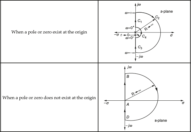
If the loop transfer function has a pole or poles at the origin in the -plane, mapping of this point will become indeterminate. Hence, a contour is taken around the origin to avoid such situations, which is shown in Fig. 9.19(b) and the zoomed view of the contour is shown in Fig. 9.19(c).

Fig. 9.19 ∣ Nyquist contour for a system with a pole and/or zero at the origin

If the mapping theorem is applied to the system, then the following conclusion is made:

If the Nyquist path for a system is chosen as shown in Fig. 9.19(a), then the number of zeros of which lies in the right half of -plane is equal to the summation of the number of poles of which lies in the right half of -plane and number of clockwise encirclements of the origin made by the contour in -plane.

9.18 Relation Between G(s) H(s)-Plane and F(s)-Plane

We know that , which is the vector sum of the unit vector and the vector . Hence, is identical to the vector drawn from the point to the point in the vector as shown in Fig. 9.20.

Therefore, encirclement of the origin by the contour in -plane is similar to the encirclement of the point by the contour in -plane. Hence, the stability of the closed-loop system can be examined by determining the number of encirclements of in -plane.

Fig. 9.20 ∣ Relationship between -plane and -plane

9.19 Nyquist Stability Criterion Based on the Encirclements of −1+ j 0

The Nyquist stability criterion based on the number of encirclements of is analyzed for two cases as below:

Case 1: When the loop transfer function has no poles or zeros on the imaginary axis

If the loop transfer function of the system has number of poles in the right half of the -plane, then for the system to be stable, the number of encirclements in the counterclockwise direction made by the locus in plane around the point must be equal to

The above criterion can be expressed as

where is the number of zeros of present in the right half of -plane, is the number of clockwise encirclements made by the locus of around the point and is the number of poles of present in the right half of -plane.

Case 2: When the loop transfer function has poles and/or zeros on the imaginary axis

If the loop transfer function has poles and/or zeros on the imaginary axis, the Nyquist path is modified by drawing a small semicircle with very small radius as shown in Fig. 9.19(c).

If the loop transfer function of the system has number of poles in the right half of the -plane, then for the system to be stable, the number of encirclements in the counterclockwise direction made by the modified locus in -plane around the point must be equal to

9.20 Stability Analysis of the System

Let be the number of zeros and be the number of poles of the characteristic equation encircled by the -plane contour (Nyquist path), then the number of encirclements, made by the -plane contour around the point in the clockwise direction can be obtained as the difference between and

i.e.,

If is negative, it implies that the encirclement is in the counterclockwise direction. The different conditions for the system to be stable are discussed in Table 9.14.

Table 9.14 ∣ Conditions for the system to be stable

In general, the condition for the closed-loop stability is that must be equal to zero and the condition for the open-loop stability is that must be equal to zero.

9.21 Procedure for Determining the Number of Encirclements

The procedure for determining the number of encirclements made by the contour in -plane around the point is given below:

Step 1: Construct the contour in -plane based on the Nyquist path in the -plane.

Step 2: Draw a dotted line from the point which is directed in the third quadrant of the -plane.

Step 3: Chose any arbitrary point in the contour in the -plane.

Step 4: Starting from the point traverse the contour in the -plane.

Step 5: If the dotted line is cut by the contour in the clockwise direction, the number of encirclements is increased by one and if the dotted line is cut by the contour in the counterclockwise direction, the number of encirclements is decreased by one.

Step 6: Repeat the above step until the arbitrary point reaches the initial position.

Step 7: The value of present at the end of one complete rotation gives the number of encirclements made by the contour in -plane around the point .

The number of encirclements made by the different contours in -plane is listed in Table 9.15.

Table 9.15 ∣ Number of encirclements for different contour in -plane

9.21.1 Flow chart for Determining the Number of Encirclements Made by the Contour in G(s)H(s)-Plane

The flow chart for determining the number of encirclements made by the contour in -plane is shown in Fig. 9.21.

Fig. 9.21 ∣ Flow chart for number of encirclements

9.22 General Procedures for Determining the Stability of the System Based on Nyquist Stability Criterion

Step 1: Construct the Nyquist path that covers the whole right-hand side of the -plane based on the loop transfer function. The different Nyquist paths for different loop transfer functions are shown below:

Step 2: Divide the Nyquist path into different sections with the value of and radius of the semi-circular path.

Step 3: For each section present in the Nyquist path, determine the contour in the -plane.

Step 4: The intersection point of the contour on the real axis is determined by substituting at which the imaginary part of the transfer function is zero.

Step 5: Complete the contour in the -plane for the given system by joining the individual contours determined in the previous step.

Step 6: Determine the number of encirclements made by the contour in -plane around the point .

Step 7: For the given loop transfer function, determine the number of poles existing in the right half of the -plane.

Step 8: Determine the number of zeros, existing in the right half of the -plane by using .

Step 9: Using Table 9.15, examine the closed-loop stability of the system.

9.22.1 Flow chart for Determining the Stability of the System Based on Nyquist Stability Criterion

The flow chart for determining the stability of the system based on Nyquist stability criterion is shown in Fig. 9.22.

Fig. 9.22 ∣ Flow chart for examining the stability of the system

Solution:

1. In general, the Nyquist path for a system is considered to have a complete right-hand side of the -plane covering the entire imaginary axis including the origin. In addition, the Nyquist path should not pass through any poles and/or zeros on the imaginary axis.

   As the pole at the origin for the given system exists, a small semicircle with infinitesimal radius is drawn around the origin of the Nyquist path. The modified Nyquist path for the system is shown in Fig. E9.6(a).

   

   Fig. E9.6(a)

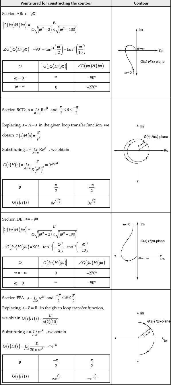
2. The different sections present in Fig. E9.6(a) alongwith its parameters are listed in Table E9.6(a).

   Table E9.6(a) ∣ Sections present in the Nyquist path

   
3. Construct a contour in -plane for each section given in Table E9.6(a) and the individual contours are listed in Table E9.6(b).

   Table E9.6(b) ∣ Contours for different sections

   
4. To determine the intersection point of the contour in the real axis:

   The loop transfer function of the given system is

   Therefore,

   

   

   Hence, the real part of the transfer function =

   and the imaginary part of the transfer function =

   Equating the imaginary part of the above transfer function to zero, we obtain

   

   or

   Substituting in the real part of the transfer function, we obtain the intersection point as .

5. The individual contours obtained in step (iii) are combined together to construct the complete contour in -plane alongwith the intersection point as shown in Fig. E9.6(b).
   

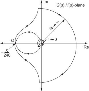
   Fig. E9.6(b)

6. The number of encirclements made by the contour in -plane around the point for the given system cannot be determined as the intersection point depends on the gain .
7. For the given system, the number of poles which lies in the right half of the -plane is zero, i.e., .
8. The number of zeros which lies in the right half of the -plane cannot be determined for the given system.
9. Hence, the stability of the system depends on the gain .
10. To determine the range of gain for the system to be stable:

    For the system to be stable, should be less than −1

    i.e., or

    Therefore, for the system to be stable, the range of gain is .

Solution:

1. As there exists no pole on the imaginary axis for the given system, the Nyquist path for the original system is shown in Fig. E9.7(a).
   

   Fig. E9.7(a)

2. The different sections present in Fig. E9.7(a) alongwith parameters are listed in Table E9.7(a).

   Table E9.7(a) ∣ Sections present in the Nyquist path

   
3. Construct a contour in -plane for each section given in Table E9.7(a) and the individual contours are listed in Table E9.7(b).

   Table E9.7(b) ∣ Contours for different sections

   
4. To determine the intersection point of the complete contour in the real axis:

   The loop transfer function of the given system is

   

   Therefore,

   =

   

   

   Hence, the real part of the transfer function =

   and the imaginary part of the transfer function =

   Equating the imaginary part of the transfer function to zero, we obtain

   

   or .

   Substituting in the real part of the transfer function, we obtain the intersection point as

   

5. The individual contours obtained in step (iii) are combined together to construct the complete contour in -plane alongwith the intersection point as shown in Fig. E9.7(b).
   

   Fig. E9.7(b)

6. The number of encirclements made by the contour in -plane around the point for the given system is 0, i.e., .
7. For the given system, the number of poles which lies in the right half of the -plane is zero, i.e., .
8. The number of zeros which lies in the right half of the -plane is determined by using .
9. Using Table 9.15 and the value of obtained in the previous step, we may conclude that the system is stable.

Solution:

1. As two poles exist at the origin for the given system, the Nyquist path for the system is shown in Fig. E9.8(a).
   

   Fig. E9.8(a)

2. The different sections present in Fig. E9.8(a) alongwith its parameters are listed in Table E9.8(a).

   Table E9.8(a) ∣ Sections present in the Nyquist path

   
3. Construct a contour in -plane for each section given in Table E9.8(a) and the individual contours are listed in Table E9.8(b).

   Table E9.8(b) ∣ Contours for different sections

   
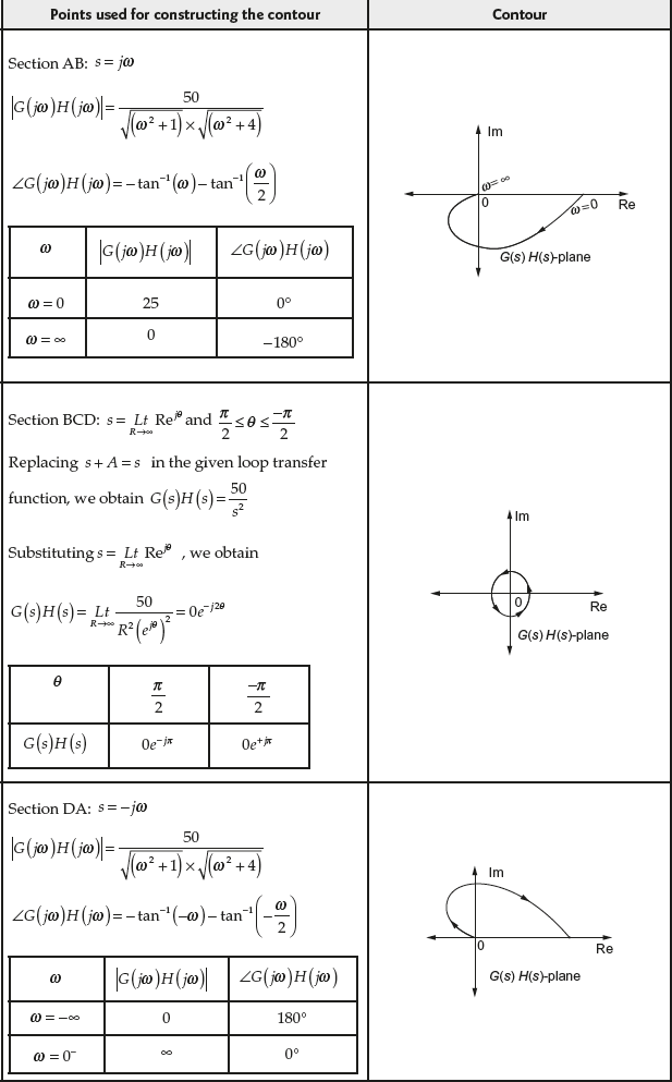
4. To determine the intersection point of the complete contour in the real axis:

   The loop transfer function of the given system is

   Therefore,

   =

   

   

   Hence, the real part of the transfer function =

   and the imaginary part of the transfer function =

   Equating the imaginary part of the transfer function to zero, we obtain .

   Substituting in the real part of the transfer function, we obtain the intersection point . Hence, there is no valid intersection point of contour on the imaginary axis.

5. The individual contours obtained in step (iii) are combined together to construct the complete contour in -plane as shown in Fig. E9.8(b).
   

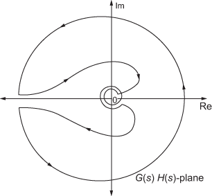
   Fig. E9.8(b)

6. The number of encirclements made by the contour in -plane around the point for the given system is 2, i.e., .
7. For the given system, the number of poles which lies in the right half of the -plane is 0, i.e., .
8. The number of zeros which lies in the right half of the -plane is determined by using .
9. Using the Table 9.15 and the value of obtained in the previous step, we may conclude that the system is unstable.

Solution:

1. As no pole exists at the origin for the given system, the Nyquist path for the system is shown in Fig. E9.9(a).
   

   Fig. E9.9(a)

2. The different sections present in Fig. E9.9(a) alongwith its parameters are listed in Table E9.9(a).

   Table E9.9(a) ∣ Sections present in the Nyquist path

   
3. Construct a contour in -plane for each section given in Table E9.9(a) and the individual contours are listed in Table E9.9(b).

   Table E9.9(b) ∣ Contours for different sections

   
4. To determine the intersection point of the contour in the real axis:

   The loop transfer function of the given system is

   Therefore,

   

   

   Hence, the real part of the transfer function =

   and the imaginary part of the transfer function =

   Equating the imaginary part of the above transfer function to zero, we obtain

   

   Substituting in the real part of the transfer function, we obtain the intersection point as . Hence, other than the point , we have no intersection of the contour in the -plane.

5. The individual contours obtained in step (iii) are combined together to construct the complete contour in -plane alongwith the intersection point as shown in Fig. E9.9(b).
   

   Fig. E9.9(b)

6. The number of encirclements made by the contour in -plane around the point for the given system is zero, i.e.,
7. For the given system, the number of poles which lies in the right half of the -plane is zero, i.e., .
8. The number of zeros which lies in the right half of the -plane is .
9. As the value of zero which lies in the right half of the -plane is zero, the system is stable.

Solution:

1. As no pole exists at the origin for the given system, the Nyquist path for the system is shown in Fig. E9.10(a).
   

   Fig. E9.10(a)

2. The different sections present in Fig. E9.10(a) alongwith its parameters are listed in Table E9.10(a).

   Table E9.10(a) Sections present in the Nyquist path

   
3. Construct a contour in -plane for each section given in Table E9.10(a) and the individual contours are listed in Table E9.10(b).

   Table E9.10(b) Contours for different sections

   
4. To determine the intersection point of the contour in the real axis:

   The loop transfer function of the given system is

   Therefore,

   

   Hence, the real part of the transfer function =

   and the imaginary part of the transfer function =

   Equating the imaginary part of the above transfer function to zero, we obtain .

   Substituting in the real part of the transfer function, we obtain the intersection point as . Therefore, the contour crosses the real axis only at .

5. The individual contours obtained in step (iii) are combined together to construct the complete contour in -plane alongwith the intersection point as shown in Fig. E9.10(b).
6. The number of encirclements made by the contour in -plane around the point for the given system is zero, i.e., .
7. For the given system, the number of poles which lies in the right half of the -plane is zero, i.e., .
8. The number of zeros which lies in the right half of the -plane is .
9. As the value of zero which lies in the right half of the -plane is zero, the system is stable.
   

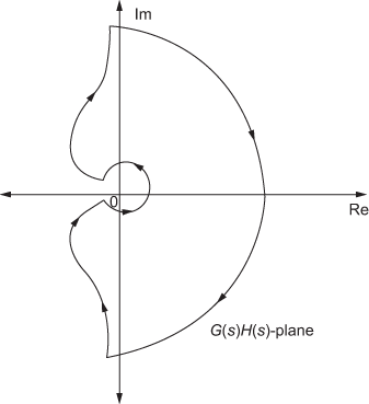
   Fig. E9.10(b)

Solution:

1. As two poles exist at the origin for the given system, the Nyquist path for the system is shown in Fig. E9.11(a).
   

   Fig. E9.11(a)

2. The different sections present in Fig. E9.11(a) alongwith its parameters are listed in Table E9.11(a).

   Table E9.11(a) ∣ Sections present in the Nyquist path

   
3. Construct a contour in -plane for each section given in Table E9.11(a) and the individual contours are listed in Table E9.11(b).

   Table E9.11(b) ∣ Contours for different sections

   
4. To determine the intersection point of the contour in the real axis:

   The loop transfer function of the given system is

   We know that when the contour crosses the real axis, the phase angle of the system will be .

   Hence,

   

   

   Taking on both sides of the equation, we obtain

   

   We know that,

   Using the above equation, we obtain

   Upon solving, we obtain

   rad/sec

   Substituting in the magnitude of the transfer function, we obtain

   

   Therefore, the contour intersects the real axis at

5. The individual contours obtained in step (iii) are combined together to construct the complete contour in -plane alongwith the intersection point as shown in Fig. E9.11(b).
   

   Fig. E9.11(b)

6. The number of encirclements made by the contour in -plane around the point for the given system is zero, i.e., .
7. For the given system, the number of poles which lies in the right half of the -plane is zero, i.e., .
8. The number of zeros which lies in the right half of the -plane is .
9. As the value of zero which lies in the right half of the -plane is zero, the system is unstable.

Solution:

1. As three poles exist at the origin for the given system, the Nyquist path for the system is shown in Fig. E9.12(a).
   

   Fig. E9.12(a)

2. The different sections present in Fig. E9.12(a) alongwith its parameters are listed in Table E9.12(a).

   Table E9.12(a) ∣ Sections present in the Nyquist path

   
3. Construct a contour in -plane for each section given in Table E9.12(a) and the individual contours are listed in Table E9.12(b).

   Table E9.12(b) ∣ Contours for different sections

   
4. To determine the intersection point of the contour in the real axis:

   The loop transfer function of the given system is

   Therefore,

   

   

   Hence, the real part of the transfer function =

   and the imaginary part of the transfer function = .

   Equating the imaginary part of the transfer function, we obtain

   

   Substituting in the real part of the transfer function, we obtain the intersection point Q as .

5. The individual contours obtained in step (iii) are combined together to construct the complete contour in -plane alongwith the intersection point as shown in Fig. E9.12(b).
   

   Fig. E9.12(b)

6. The number of encirclements made by the contour in -plane around the point for the given system cannot be determined as the intersection point depends on the gain .
7. For the given system, the number of poles which lies in the right half of the -plane is zero, i.e., .
8. The number of zeros which lies in the right half of the -plane cannot be determined for the given system.
9. As the value of zero which lies in the right half of the -plane is not determined, the stability of the system cannot be analyzed. The stability of the system depends on the .
10. To determine the range of gain for the system to be stable:

    For the system to be stable, should be less than −1.

    i.e., or

    Therefore, for the system to be stable, the range of gain is .

Solution:

1. As no poles exist at the origin for the given system, the Nyquist path for the system is shown in Fig. E9.13(a).
   

   Fig. E9.13(a)

2. The different sections present in Fig. E9.13(a) alongwith parameters are listed in Table E9.13(a).

   Table E9.13(a) ∣ Sections present in the Nyquist path

   
3. Construct a contour in -plane for each section given in Table E9.13(a) and the individual contour is listed in Table E9.13(b).

   Table E9.13(b) ∣ Contour for different sections

   
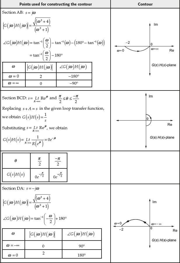
4. To determine the intersection point of the contour in the real axis:

   The loop transfer function of the given system is

   Therefore,

   Hence, the real part of the transfer function =

   and the imaginary part of the transfer function = .

   Equating the imaginary part of the transfer function, we obtain .

   As the real part of the transfer function is independent of , there is no intersection point on the real axis other than −2.

5. (v) The individual contours obtained in step (iii) are combined together to construct the complete contour in -plane alongwith the intersection point as shown in Fig. E9.13(b).
6. The number of encirclements made by the contour in -plane around the point for the given system is .
7. For the given system, the number of poles which lies in the right half of the -plane is zero, i.e., .
8. The number of zeros which lies in the right half of the -plane for the given system is .
9. As the value of zero which lies in the right half of the -plane is zero the given system is stable.

Fig. E9.13(b)

Review Questions

1. A feedback control system is characterized by the open-loop transfer function
   1. Draw the polar plot of the open-loop system. Calculate the magnitude and phase at 10 equi-spaced frequency points, including the point where the plot intersects the imaginary axis and use them to construct the plot.
   2. From the polar plot, how will you determine the gain margin, phase margin, gain crossover frequency and phase crossover frequency? Comment on the system stability.
2. Draw the polar plot of each of the following complex functions:
   1. 
   2. 
   3. 
   4. 
3. Sketch the polar plot for , .
4. Determine: (a) the phase crossover frequency, (b) the gain crossover frequency, (c) the gain margin and (d) phase margin for the system of with and
5. Sketch the polar plot for
   1. 
   2. 
   3. 
   4. 
   5. 
   6. 
   7. 
   8. 
   9. 
   10. 
   11. 
   12. 
   13. 
   14. 
   15. 
6. Sketch the polar plot for the following loop transfer function (a) and (b) .
7. Draw the polar plot for the unity feedback system given by and determine the range of for the stability of the system.
8. Sketch the polar plot for the unity feedback system given by and find the phase margin.
9. Draw the polar plot for the transfer function of a system .
10. Consider the transfer function Draw the polar plot for
11. Consider the non-minimum phase transfer function Sketch the polar plot.
12. Draw the polar plot for the transfer function
13. Consider the following transfer function Show that the polar plot of in the plane is a circle and diameter as varies from to .
14. Determine graphically the gain margin and phase margin and gain and phase crossover frequencies for the system whose open-loop transfer function is given as.
15. The open-loop transfer function of a unity feedback control system is given by . Sketch the polar plot and determine the gain margin and phase margin.
16. Determine the phase margin ad gain margin for the system whose transfer function is . Use polar plot.
17. The open-loop transfer function of a unity feedback control system is given by Derive an expression for the gain in terms of and and specify the gain margin
18. Draw the polar plot for the following transfer functions (a) and (b) .
19. For the following transfer function draw the actual polar plot by calculating the magnitude and phase for
20. Determine analytically phase margin, gain margin, phase crossover frequency and gain-crossover frequency for the transfer function given below. Draw the polar plot.

    

21. Sketch the polar plot for the following transfer function:

    

22. For an RLC series network, the output is taken across the capacitor. The transfer function is where the undamped natural frequency and damping coefficient . Draw the polar plot.
23. Obtain the polar plot for the unity feedback control system having open-loop transfer function as , assume .
24. State and explain the Nyquist criterion for stability.
25. State the Nyquist stability criterion for the stability of a closed-loop system and compare it with Routh's criterion.
26. Given the open-loop transfer function , determine the condition of stability from the polar plot. Verify this condition using Routh–Hurwitz criterion.
27. Write a note on Nyquist path.
28. Define gain margin and phase margin with reference to Nyquist plot.
29. Explain clearly with the necessary mathematical preliminaries the Nyquist criterion for stability.
30. Explain the conditionally stable system. With the help of a Nyquist plot, show the behaviour of such systems.
31. What are the effects of additional poles and zeros on the shape of the Nyquist loci? Explain using appropriate diagrams.
32. Define principle of arguments.
33. Using Nyquist criterion, investigate the stability of the system
34. If a position control system has the forward loop transfer function , determine the gain margin and phase margin the system using Nyquist plot.
35. Given , determine the stability range of K using Nyquist's stability criterion.
36. The loop transfer function of a unity feedback system is given by . Sketch the polar plot for the system and determine the gain and phase margin of the system.
37. The loop transfer function of a unity feedback system is given by . Sketch the polar plot for the system and determine the gain and phase margin of the system.
38. The loop transfer function of a unity feedback system is given by . Sketch the polar plot for the system.
39. The open-loop transfer function of a feedback system is , determine its stability using Nyquist criterion.
40. Sketch the Nyquist plot for and determine whether the closed-loop system is stable or not.
41. The loop transfer function is Determine, using Nyquist stability criterion, the critical value of K for stability of closed-loop system.
42. A position control system has the forward loop transfer function . Draw the Nyquist plot and determine the stability of the closed-loop system.
43. Sketch the Nyquist plot for the system whose open-loop transfer function is given by and using Nyquist stability criterion, check whether system is stable.
44. The open-loop transfer function of a unity feedback control system is given by . Draw the Nyquist plot and calculate the gain margin.
45. The loop transfer function of a feedback system is given by . Sketch the Nyquist plot and determine the stability and hence the gain and phase margins.
46. Sketch the Nyquist plot for the following open-loop transfer function and comment on the stability . Determine the gain and phase margins.
47. A control system has the loop transfer function . Sketch the Nyquist diagram and determine its stability.
48. The loop transfer function of a feedback system is . Using Nyquist method, determine the stability of the system.