2

PHYSICAL SYSTEMS AND COMPONENTS

2.1 Introduction

Modeling is the process of obtaining a desired mathematical description of a physical ­system. The basic differential equations that may be linear or non-linear for any physical system are obtained by using appropriate laws. The differential equations thus obtained can make the analysis of the system easier. Laplace transformation tool is applied to these ­differential ­equations to get the transfer function of the physical system. In this chapter, the ­differential equations and the transfer functions for physical systems such as ­electromechanical, ­hydraulic, pneumatic, liquid level and thermal systems are obtained. The control system components such as controllers, potentiometers, synchros, servomotors, tachogenerators, stepper motor and gear trains are also discussed.

2.2 Electromechanical System

Systems that carry out electrical operations with the help of mechanical elements are known as electromechanical systems. Devices based on electromechanical systems are developed for making the energy conversion easier between electrical and mechanical systems. The subsystems present in the electromechanical systems are shown in Fig. 2.1.

Fig. 2.1 ∣ Subsystems in electromechanical systems

For an electromechanical system, voltages and currents are used to describe the state of its electrical subsystem based on Kirchhoff's laws. Position, velocity and ­accelerations are used to describe the state of its mechanical subsystems based on Newton's law. The magnetic subsystem or magnetic field acts as a boat in transferring and converting energy between electrical and mechanical subsystems. Magnetic flux, flux density and field strength governed by Maxwell's equations are used to describe the conversion and ­transformation processes.

Magnetic flux interacting with the electrical subsystem will produce a force or a torque on the mechanical subsystem. In addition, the movement in the mechanical subsystem will produce an induced electromotive force (emf) in the electrical subsystem. Electromotive force is developed due to the variation of the magnetic flux linked with the electrical subsystem. Therefore, the electrical energy and the mechanical energy conversions occur with the help of the magnetic subsystem.

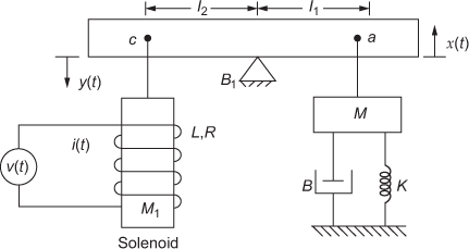
Fig. E2.1

Solution: The exciting current of solenoid is given by

This produces a force, in the solenoid where = soleniod constant in N/A.

This force,

(1)

where is the reaction force at point c.

The force acting at point a is

Equating momentum at the centre,

This gives

(2)

The fulcrum will give displacement as

Taking Laplace transform, we obtain

(3)

Substituting Eqn. (3) and Eqn. (2) in Eqn. (1), we obtain

Hence, the transfer function is given by

Solution:

Fig. E2.2

Applying Kirchhoff's voltage law, loop equations are obtained as follows:

(1)

(2)

where K₁ is a constant.

Taking Laplace transform, we obtain

(3)

(4)

Substituting Eqn. (4) in Eqn. (3), we have

From Eqn. (4), we have

(5)

Substituting Eqn. (5) in Eqn. (3), we obtain

(6)

Also, we have

Taking Laplace transform, we obtain

(7)

Substituting Eqn. (7) in Eqn. (6), we obtain

Thus, the transfer function of the given system is

2.3 Hydraulic System

Hydraulics is the study of incompressible liquids and hydraulic devices are the devices that use oil as their working medium. Since the density of the oil does not vary with pressure, it is used as a working medium in the hydraulic systems. Liquid-level systems are a class of hydraulic system. The factors such as positiveness, accuracy, flexibility, high horse power-to-weight ratio, fast starting and stopping, precision, simplicity of operation and smooth ­reversal of operation make the hydraulic system find wide applications. Hydraulic system that is non-linear in nature is stable and satisfactory under all the ­operating conditions.

The operating pressure of hydraulic systems is between 1 and 35 MPa. It varies based on the application. The weight and size of the hydraulic system vary inversely with respect to the supply pressure for the same power requirement. A very high driving force for an application can be obtained by using high-pressure hydraulic systems. Due to the advantages of electronic control and hydraulic power, the electronic system in combination with the hydraulic system is widely used.

2.3.1 Advantages of Hydraulic System

The advantages of hydraulic system are:

1. The fluid (oil) used in the hydraulic system acts as a lubricant.
2. Fluid in the system is used to carry the heat generated conveniently to the heat exchanger.
3. Hydraulic devices have higher speed of response.
4. Hydraulic actuators can be operated at different conditions without damage (continuous, intermittent, reversing and stalled condition).
5. Flexibility exists in the design, due to the availability of linear and rotary actuators.
6. When loads are applied, the speed drop is small due to the presence of low leakage in the actuators.

2.3.2 Disadvantages of Hydraulic System

The disadvantages of hydraulic system are:

1. Cost of a hydraulic system is higher when compared to an electrical system.
2. Occurrence of fire and explosion due to the usage of non-fire-resistant liquids.
3. Difficult to maintain the system due to the presence of leakage.
4. Failure occurs in the system due to the presence of contaminated oil.
5. Availability of hydraulic power is less when compared to electrical power.
6. Difficult to design the sophisticated hydraulic system due to the involvement of non-linear and complex characteristics.
7. Has poor damping characteristics.

2.3.3 Applications of Hydraulic System

Hydraulic system is widely used in the control applications such as power steering and brakes in automobiles, steering mechanisms of large ships, control of large machine tools, etc.

2.3.4 Devices Used in Hydraulic System

Devices such as dashpots, pumps and motors, valves, linear actuator, servo systems, feedback systems and controllers are used in hydraulic systems.

Fig. E2.3

Solution: Let the pressure existing on the left and right sides of the piston be and respectively. If the inertia force is taken as a negligible quantity, then the force existing on the piston should balance the spring force. Then,

where A is the piston area in m² and k is the spring constant in kg/m.

The flow rate of oil through the resistance R is given by

where is the flow rate of oil though resistance in kg/sec and R is the resistance to the flow of oil in .

The flow of oil through the resistance during dt seconds must be equal to the change in mass of oil to the right of the piston during the same dt seconds. Therefore,

where is the density of oil.

Therefore,

Substituting the value of q(t) in the above equation and solving, we get

Taking Laplace transform, we obtain

Thus, the transfer function of the system is given by

where with the dimension of time.

2.4 Pneumatic Systems

In pneumatic systems, the compressible fluid that is used as a working medium is air or gas. The pneumatic system is most frequently used in industrial control system due to the fact that it provides a greater force than the force obtained from electrical devices. In ­addition, it provides more safety against fire accidents. The dynamic equations for modeling of ­pneumatic systems are obtained using conservation of mass. The devices in the pneumatic systems involve with the flow of air or gas through connected pipe lines and pressure vessels. The variables involved in the pneumatic systems are mass flow rate and pressure P. The electrical analogous variables to the mass flow rate and pressure are current and ­voltage respectively.

2.4.1 Gas Flow Resistance and Pneumatic Capacitance

The basic elements of the pneumatic systems are resistance and capacitance. The resistance to gas flow is due to the restrictions present in the pipes and valves. Hence, the gas flow resistance R is defined as the ratio of rate of change in gas pressure to the change in the gas flow rate.

The pneumatic capacitance C of a pressure vessel depends on the type of expansion involved. The pneumatic capacitance of a pressure vessel is defined as the ratio of change in gas stored to the change in gas pressure.

2.4.2 Advantages of Pneumatic System

The advantages of pneumatic system are:

1. The working medium used in the pneumatic systems is non-inflammable and offers safety from fire hazards.
2. Viscosity of gas or air is negligible.
3. Return pipelines are not necessary since the air or gas can be exhausted once the working cycle of device comes to an end.

2.4.3 Disadvantages of Pneumatic System

The disadvantages of pneumatic system are:

1. Response of the pneumatic system is slower since the working medium is ­compressible.
2. Power output of the pneumatic system is less.
3. Accuracy of the actuator in the system is less.

2.4.4 Applications of Pneumatic System

Pneumatic system is used in guided missiles, air craft systems, automation of production machinery and automatic controllers in many fields.

2.4.5 Devices Used in Pneumatic System

Devices such as bellows, flapper valve, relay, actuator, position control system and controllers are used in pneumatic systems.

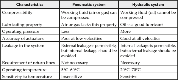
2.4.6 Comparison between Hydraulic and Pneumatic Systems

The comparison of hydraulic and pneumatic systems based on the common characteristics between the systems is given in Table 2.1.

Table 2.1 ∣ Pneumatic system vs hydraulic system

Fig. E2.4

Solution: Consider that is the steady-state value of pressure in the system, is the small deviation in the input pressure and is the small deviation in the output pressure.

For small deviation in the input and output pressures, the gas flow resistance R can be obtained as

and the pneumatic capacitance C can be obtained as

where m is the mass of gas in the device and q is the gas flow rate.

Since the product of pressure change and the capacitance C is equal to the gas added to the vessel during dt seconds, we obtain

Therefore,

Taking Laplace transform, we obtain

Hence, the transfer function of the system relating the change in input pressure and output pressure is given by

Fig. E2.5

Solution: Let be the steady-state value of input pressure,

be the small increment in the input pressure,

be the small increment in the air flow,

be the small increment in the pressure existing inside the bellow and

be the displacement of the movable surface due to increase in pressure.

The force on the movable surface is proportional to the pressure inside the bellow and is given by

where A is the area of the bellow.

Also, the force opposing the movement of the flat surface of bellow walls is proportional to the displacement and is given by

where K is the stiffness of the bellow.

At steady state, the above-said forces are in a balanced condition

Therefore, (1)

The gas flow resistance R is given by

(2)

The pneumatic capacitance C is given by

Therefore, (3)

Using Eqs. (2) and (3), we obtain

Therefore, (4)

Using Eqn. (1) and Eqn. (4), we obtain

Taking Laplace transform, we obtain

Hence, the transfer function of the system is given by

where is the time constant of the system.

2.5 Thermal Systems

Systems involving the transfer of heat from one substance to another are known as thermal systems. Thermal systems can be modeled by knowing the basic elements involved in the systems. The basic elements in a thermal system are thermal resistance and thermal capacitance that are distributed in nature. But, for the analysis of thermal systems, the nature of the basic elements is assumed to be lumped. The assumption made in the lumped parameter model is that, the substances that are characterized by resistance to heat flow have negligible capacitance and vice versa.

The different ways by which the heat flows from one substance to another substance are conduction, convection and radiation. The heat flow rate for different ways is:

For conduction or convection,

Heat flow rate

where is the heat flow rate in kcal/sec, is the coefficient in kcal/sec ^oC and is the temperature difference in degree Celsius.

The coefficient is given by

where is the thermal conductivity in kcal/m sec ^oC, is the area normal to heat flow in m²_, is the thickness of conductor in m and is the convection coefficient in kcal/m² sec ^oC.

For radiation,

Heat flow rate,

If , then

where is the radiation coefficient in kcal/sec ^oC.

Effective temperature difference =

In this section, we consider that the heat flow is through conduction and convection.

2.5.1 Thermal Resistance and Thermal Capacitance

Thermal resistance for heat transfer between two substances is given by the ratio of change in temperature to the change in heat flow rate.

For conduction and convection,

Since thermal coefficient for conduction and convection is almost constant, thermal resistance is also constant for conduction and convection.

Thermal capacitance is given by the ratio of change in heat stored to change in ­temperature.

or

where is the mass of substance considered in kilogram and is the specific heat of substance in kcal/kg °C.

Fig. E2.6

Solution: Let be the steady-state temperature of input liquid in °C,

be steady-state temperature of output liquid in °C,

be liquid flow rate in steady state in kg/sec,

M be the mass of liquid in kg,

c be the specific heat of liquid in kcal/kg °C,

R be the thermal resistance in °C − sec/kcal and

C be the thermal capacitance in kcal/°C.

be the input heat rate in steady state in kcal/sec.

If the change in input heat rate is , there will be change in the output heat rate and is given by . In addition, the temperature of the out-flowing liquid will also be changed and is given by .

The equation for the system shown in Fig. E2.6 is obtained as

= Rate of flow of liquid specific heat of liquid c change in temperature

i.e., (1)

Thermal capacitance C = mass M specific heat of liquid c

i.e., C = Mc(2)

Thermal resistance

i.e., (3)

Substituting Eqn. (1) in Eqn. (3), we obtain

(4)

For the given system, the rate of change of temperature is directly proportional to change in input heat rate.

Therefore,

(5)

Substituting Eqn. (3) in the above equation, we obtain

Taking Laplace transform, we obtain

Hence, the transfer function of the given system is

Fig. E2.7

Solution: Assume that, the small change in liquid temperature and change in temperature as indicated by thermometer are and respectively.

Hence, the heat stored in thermometer is given by

and heat transmitted is given by

Since the net heat equals to zero, the system equation can be written as

Taking Laplace transform, we obtain

Rearranging the above equation, we obtain the transfer function of the system as

Taking inverse Laplace transform, we obtain

The above equation shows the variation in thermometer as a time function.

2.6 Liquid-Level System

Liquid-level system in any industrial process involves the flow of liquid through connecting pipes and storage tanks. The flow of liquid can be generally classified as laminar and turbulent flow depending on the magnitude of Reynolds number. If the Reynolds number is less than 2,000, then the flow is laminar; else if the Reynolds number is greater than 3,000 and less than 4,000, the flow is turbulent. But, in any industrial process involving the flow of liquid, the flow is often turbulent and not laminar.

In liquid-level control system, the height of the liquid in tanks and the flow rate of the liquid in pipes are the variables that ought to be controlled. Liquid-level system can be represented either by linear or non-linear differential equations depending on the type of flow of liquid. If the flow of liquid is laminar, the system will be represented by linear differential equations and if the flow is turbulent, the system is represented by non-linear differential equations.

2.6.1 Elements of Liquid-Level System

Resistance and capacitance of liquid-level systems describe the dynamic characteristic of the system. The resistance of the liquid is defined by assuming that the flow of liquid is through a short pipe connecting two tanks. The resistance R is defined as the change in liquid-level between two tanks necessary to cause a unit change in flow rate.

The relationship between the flow rate and the level difference differs for the laminar and turbulent flow and hence the resistance value also differs between the two.

Resistance for laminar flow

Resistance for turbulent flow

where H is the steady-state head in m and Q is the steady-state liquid flow rate in m³/sec.

Capacitance C of a tank is defined to be the change in quantity of stored liquid that is necessary to cause a unit change in potential (head).

The analogous quantities for different physical system to electrical system are given in Table 2.2.

Table 2.2 ∣ Analogous quantities of different physical system to electrical systems

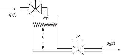
Fig. E2.8

Solution: The variables indicated in the system shown in Fig. E2.8 are defined by

inflow rate of liquid in

outflow rate of liquid in

height of liquid in m

Under steady-state conditions, we obtain

steady-state flow rate

steady-state liquid level in tank

If there is a small increase in the inflow rate, there will be two changes occurring in the liquid-level system as follows:

1. Increase in the liquid level of the tank.
2. Increase in the outflow of the liquid.

From the definition of resistance,

(1)

Using liquid flow rate balance equation, we obtain

Liquid inflow − liquid outflow = rate of liquid storage in the tank

(2)

Substituting Eqn. (1) in Eqn. (2), we obtain

Therefore, (3)

where C is the capacitance of tank and R is the resistance of the outlet pipe.

Therefore,

Taking Laplace transform, we obtain

Therefore,

If is taken as the input and the output, the transfer function of the system is given by

But, if is taken as the output, the transfer function is obtained as follows:

Differentiating Eqn. (1), we obtain

(4)

Substituting Eqn. (4) in Eqn. (2), we obtain

Taking Laplace transform, we obtain

Thus, the transfer function of the system is given by

2.7 Introduction to Control System Components

The basic components present in a typical closed-loop control system are shown in Fig. 2.2.

Fig. 2.2 ∣ Block diagram of a typical control system

The basic components present in the control system are the error detector, amplifier, controller, actuator, plant and sensor or feedback system. Controller is the block that combines the error detector, amplifier and controller. The control system shown in Fig. 2.2 will become an open-loop system in the absence of automatic controller unit.

Error detector produces an error signal that is the difference between the reference input and the feedback signal . The devices that can be used as error-detecting units are potentiometer, linear variable differential transformer (LVDT), synchros, etc.

Amplifier amplifies the error signal so that the controller can modify the error signal to have better control action over the plant or system. In general, in many control systems, controller itself amplifies the error signal.

Controller amplifies the signal produced by the amplifier unit to produce a control ­signal to stabilize the system. Depending on the nature of error signal/signal from amplifier, the controller used in the control system may be electrical, electronic, hydraulic or pneumatic controllers. The controller may be either proportional (P) controller, proportional integral (PI) controller, proportional derivative (PD) controller and proportional integral ­derivative (PID) controller. Electrical/electronic controllers are used when the error signal/amplifier output is electrical and the controllers are designed using RC circuit/operational amplifiers. Similarly hydraulic/pneumatic controllers are used when the error signal/amplifier output is mechanical and the controllers are designed using hydraulic servomotors/pneumatic flapper valves.

Actuator is an amplifier that amplifies the controller output and converts the signal into the form that is acceptable by the plant. The devices that can be used in an actuator are pneumatic motor/valve, hydraulic motor/electric motors (DC servomotor and stepper motor)

Feedback system generates a feedback signal proportional to the present output and converts it to an appropriate signal that can be used by the error detector. The devices that can be used for generating the appropriate signal from the present output are transducers, tachogenerators, etc.

2.8 Controllers

A controller is an important component in the control system that produces the control ­signal by modifying the error signal. In addition, the controller modifies the transient response of the system. The action taken up by the controller in the control system is known as control action.

2.8.1 Controller Output as a Percentage Value

In a closed-loop control system, as a particular controller model can be used for many ­processes, the measurement variable cannot be anticipated in advance to have controller action. For example, a particular model can be used in temperature-control application as well as in the motor control. Hence, the input and output values of a particular system can be expressed in percentage rather than in its actual unit to determine percentage of ­controller output to have the desired value as output from the system. The controller output in ­percentage can be expressed as

where 0% is the minimum controller output and 100% is the maximum controller output.

2.8.2 Measured Value as a Percentage Value

In a closed-loop control system, as the unit of measured value and reference input are ­different, it is convenient to express the measured value and set point as a percentage value to make the error calculation easier. The measured value in percentage can be expressed as follows:

2.8.3 Set Point as a Percentage Value

In a closed-loop control system, the set point can be expressed as a percentage value to make the error calculation easier. The set point in percentage can be expressed as

2.8.4 Error as a Percentage Value

In a closed-loop system, the error in percentage can be expressed if the set point (SP) and measured value (MV) are expressed as percentage values. Therefore,

Solution: The operating range of the speed control for a motor = (1,600−150) rpm = 1,450 rpm.

1. 

   = = 51.72%.

2. 

   = = 50%

   Error for the given speed control of a motor = SP − MV = 900 − 875 = 25 rpm

1. = 51.72%−50% = 1.72%

   Also,

   = = 1.72%

2.8.5 Types of Controllers

In general, controllers are classified as (i) analog controllers, (ii) digital controllers and (iii) fuzzy controllers.

1. Analog controllers are further classified as follows:
   1. ON–OFF controller
   2. Proportional controller
   3. Integral controller
   4. Derivative controller
   5. Proportional Derivative controller
   6. Proportional Integral controller
   7. Proportional Integral Derivative controller
2. (ii) Digital Controller

   Initially, digital controller was implemented to perform analog controllers operation by using computers. But nowadays, due to the advancement of digital controller over ­analog ­controllers, they have been widely used to control the system. The simple block diagram of a digital controller is shown in Fig. 2.3.

   

   Fig. 2.3 ∣ Block diagram of digital controller

   Here, an analog error signal is converted into digital signal using analog-to-digital (A/D) conversion. The converted error signal is processed by a digital algorithm to give a manipulated variable in digital form. The manipulated variable in digital form will be converted to the required form using digital-to-analog (D/A) conversion.

   Advantages of digital controller are:

   1. inexpensive
   2. easy to configure and reconfigure through software
   3. scalable
   4. adaptable
   5. less prone to environmental conditions
3. (iii) Fuzzy Controller

   Fuzzy controller is the advanced form of digital controller where the control algorithms are implemented using fuzzy sets. The block diagram of a fuzzy controller is shown in Fig. 2.4.

   

   Fig. 2.4 ∣ Block diagram of fuzzy controller

It consists of an input filter, fuzzy system and an output filter. The input filter maps the sensor or error signals to the appropriate signal to be used by the fuzzy system. The fuzzy system contains the control strategy to be implemented to the output of the input filter to produce the manipulated variable. Fuzzy system executes the appropriate rule and generates a result for each. Finally, the output filter converts the fuzzy system output to a specific control output value. Power sources used in the controllers are electricity, compressed air or oil. Hence, the controller used in the control system may be classified as electrical, electronic, hydraulic or pneumatic controllers.

The controller for a particular system is decided based on the type of plant and operating conditions such as cost, availability, reliability, accuracy, weight, size and safety.

2.9 Electronic Controllers

The controllers using electrical signals and digital algorithms which perform the ­control action are known as electronic controllers. These types of controllers are used where large load changes are encountered and fast response is required. Electronic controllers are ­classified based on the control action performed by the controllers. The classification of ­controllers based on the control action is listed in Table 2.3.

Table 2.3 ∣ Control action and its respective controller

2.9.1 ON–OFF Controller

ON–OFF control is the simplest form and it drives the manipulated variable from fully closed to fully open or vice versa depending on the error signal. Due to the simplicity of the controller, it is very widely used in both industrial and domestic control system. A common example of ON–OFF control is the temperature control in a domestic heating system. When the temperature is below the thermostat set point, the heating system is switched on and when the temperature is above the set point, the heating system is switched off.

Types of ON–OFF Controller: The different ways in which the ON–OFF controller operated are

1. Two position ON–OFF controller
2. Multi-position control (floating control)

(i) Two Position ON–OFF Controller

In the two position ON–OFF controller, the output of the controller changes when the error value changes from positive to negative or vice versa. The simple electronic device that provides the ON–OFF control action is an electromagnetic relay. It has two contacts: normally open (NO) and normally closed (NC) contacts. The opening of the contact is controlled by the relay coil, which when excited changes the contact from one position to another (i.e., NONC or NCNO).

The output signal from the controller , based on the actuating error signal , may be either at a maximum or minimum value.

for

for

The block diagram of a two position ON–OFF controller is shown in Fig. 2.5.

Fig. 2.5 ∣ Block diagram of two position ON–OFF controller

Fig. 2.5 ∣ (a) Input

Fig. 2.5 ∣ (b) Relay

Fig. 2.5 ∣ (c) Output

Example of Electronic Two Position ON–OFF Controller The two-position ON–OFF ­controller implemented electronically using a comparator circuit is shown in Fig. 2.5(d).

Fig. 2.5 ∣ (d) Electronic ON–OFF controller

Neutral Zone: In practical, a differential gap exists when the controller output changes from one position to another in the two-position ON–OFF control mode of operation. The differential gap existing is known as neutral zone. Since in two-position ON–OFF controller, the controller output often switches between two positions, there exists a chattering effect that results in the premature wearing of the component. Hence, the neutral zone in the two position ON–OFF controller is used to prevent this chattering effect. In the neutral zone, the controller output will remain in its previous value. The two position ON–OFF controller with neutral zone is shown in Fig. 2.6.

Fig. 2.6 ∣ Two position ON–OFF controller with neutral zone

Application of Two-Position ON–OFF Controller The two position ON–OFF controller is used in

1. air conditioning/room heating system
2. refrigerator temperature control system
3. liquid bath temperature control
4. (d) liquid-level control in tanks

(ii) Multi-Position Control (Floating Control)

The multi-position/floating control is an extension of two-position ON–OFF control. In this control, the output from the controller can have more than two values. The ­multi-position controller reduces the controller cycling rate when compared to the two position ON–OFF controller. The most common example of multi-position control is the three position control in which the controller output can have three (0%, 50% and 100%) outputs. The ­mathematical description of three position controller is as follows:

Fig. 2.7 shows the schematic diagram of the three position controller.

Fig. 2.7 ∣ Three-position controller

The multi-position control is difficult to implement with op-amps, mechanical, ­pneumatic and hydraulic control elements as it is not as popular as two-position ON–OFF controls. Hence, the multi-position control can be implemented using microprocessor.

2.9.2 Proportional Controller

The proportional (P) controller is simple and the most widely used method of control. The proportional control is more complex than the ON–OFF control system but simpler than the conventional PID-controller. Implementation of proportional controller is simple. In proportional controller, the error signal is amplified to generate the control (output) signal. The output signal of the proportional controller , is proportional to the error signal .

In P-controller,

where is the proportional gain or constant.

Taking Laplace transform, we obtain

Therefore, the transfer function of the P-controller is given by

The block diagram of the P-controller is shown in Fig. 2.8.

Fig. 2.8 ∣ Block diagram of proportional controller

Proportional Band: The gain in the proportional controller can be referred to the proportional band. The relationship existing between the proportional band and the proportional gain is given below:

In transfer characteristics, the proportional band is used to represent the maximum ­percentage of error that will change the controller output from minimum to maximum.

When the controller output is expressed in per cent, the actual controller output can be found using

where is the actual controller output, is the transfer gain, is the controller output in per cent and is the actual output for 0% controller output.

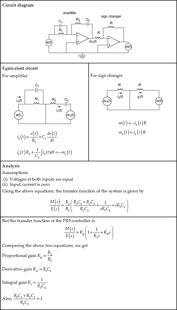
Example of Electronic P-Controller: The proportional controller can be realized either by an inverting amplifier followed by a sign changer or by a non-inverting amplifier with adjustable gain. The analysis of proportional controller using non-inverting amplifier and by using inverting amplifier is given in Table 2.4 and Table 2.5 respectively.

Table 2.4 ∣ P − Controller using non−inverting amplifier

Table 2.5 ∣ P − Controller using inverting amplifier

Advantages of P-controller

The advantages of P-controller are:

1. It amplifies the error signal by the gain value .
2. It increases the loop gain by .
3. It improves the steady-state accuracy, disturbance signal rejection and relative ­stability.
4. The use of controller makes the system less sensitive to parameter variations.

Disadvantages of P-controller

The disadvantages of P-controller are:

1. System becomes unstable if the gain of the controller increases by large value.
2. P-controller leads to a constant steady-state error.

2.9.3 Integral Controller

The integral (I) controller relates the present error value and the past error value to determine the controller output. The output signal of the integral controller is proportional to integral of the input error signal .

In I-controller,

where is the integral gain or constant.

Taking Laplace transform, we obtain

Therefore, the transfer function of the I-controller is given by

The block diagram of the I-controller is shown in Fig. 2.9.

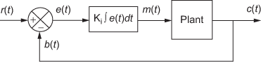
Fig. 2.9 ∣ Block diagram of an integral controller

The integral controller is used alongwith the proportional controller to form the ­PI-controller or alongwith proportional derivative controller to form the PID controller.

Example of Electronic I-Controller: The integral controller can be realized by an integrator using op-amp followed by a sign changer. The analysis of such an electronic I-controller is given in Table 2.6.

Table 2.6 ∣ I-Controller using op-amp

Advantages of I-controller

The advantages of I-controller are:

1. It reduces the steady-state error without the help of manual reset. Hence, the controller is also called as automatic reset.
2. It eliminates the error value.
3. It eliminates the steady-state error.

Disadvantages of I-controller

The disadvantages of I-controller are:

1. Action of this controller leads to oscillatory response with increased or decreased amplitude, which is undesirable and the system becomes unstable.
2. It involves integral saturation or wind-up effect.
3. There is poor transient response.

2.9.4 Derivative Controller

The derivative controller (D-controller) is also known as a rate or anticipatory controller. The controller output of the derivative controller is dependent and is proportional to the differentiation of the error with respect to time. The output signal of the integral controller is proportional to integral of the input error signal .

In D-controller,

where is the derivative gain or constant.

Taking Laplace transform, we obtain

Therefore, the transfer function of the D-controller is given by

The block diagram of the D-controller is shown in Fig. 2.10.

Fig. 2.10 ∣ Block diagram of Derivative controller

Example of Electronic D-Controller: The derivative controller can be realized by a differentiator using op-amp followed by a sign changer. The analysis of such an electronic ­D-controller is given in Table 2.7.

Table 2.7 ∣ D-controller using op-amp

Advantages of D-controller

The advantages of D-controller are:

1. Feed forward control
2. Resists the change in the system
3. Has faster response
4. Anticipates the error and initiates an early corrective action that increases the ­stability of the system
5. Effective during transient period

Disadvantages of D-controller

The disadvantages of D-Controller are:

1. Steady-state error is not recognized by the controller even when the error is too large.
2. This controller cannot be used separately in the system.
3. It is mathematically more complex than P-control.

2.9.5 Proportional Integral Controller

The individual advantages of proportional and integral controller can be used by combining the both in parallel, which results in the PI-controller. The output of the proportional integral controller (PI-controller) consists of two terms: one proportional to error signal and the other proportional to the integral of error signal.

In PI-controller,

where is the proportional gain and is the integral gain.

Taking Laplace transform, we obtain

The transfer function of the PI-controller is given by

The block diagram of PI-controller is shown in Fig. 2.11.

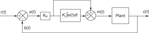
Fig. 2.11 ∣ Block diagram of PI-controller

The equivalent block diagram of the PI controller is shown in Fig. 2.12.

Fig. 2.12 ∣ Equivalent block diagram of PI-controller

Example of Electronic PI-Controller: The PI-controller can be realized by an op-amp integrator with the gain followed by a sign changer. The analysis of such an electronic PI-controller is given in Table 2.8.

Table 2.8 ∣ PI − controller using op-amp

Advantages of PI-controller

The advantages of PI-Controller are:

1. Eliminates the offset present in the proportional controller
2. Provides faster response than the integral controller due to the presence of proportional controller also.
3. Fluctuation of the system around the set point is minimum
4. Has zero steady state error
5. Form of a feedback control
6. Increases the loop gain

Disadvantages of PI-controller

The disadvantages of PI-controller are:

1. It has maximum overshoot.
2. Settling time is more.

2.9.6 Proportional Derivative Controller

The proportional derivative (PD) controller is used in the system to have faster response from the controller. It combines the proportional and derivative controller in parallel. The output of the proportional derivative controller consists of two terms: one proportional to error signal and the other proportional to the derivative of error signal.

In PD controller,

Therefore,

where is the proportional gain and is the derivative gain.

Taking Laplace transform, we obtain

Therefore, the transfer function of the PD-controller becomes

The block diagram of PD-controller is shown in Fig. 2.13.

Fig. 2.13 ∣ Block diagram of PD-controller

The equivalent block diagram of PD controller is shown in Fig. 2.14.

Fig. 2.14 ∣ Equivalent block diagram of PD-controller

Example of Electronic PD-Controller The PD-controller can be realized by an op-amp differentiator with the gain followed by a sign changer. The analysis of such an electronic PD-controller is given in Table 2.9.

Table 2.9 ∣ PD − controller using op-amp

Advantages of PD-controller

The advantages of PD-controller are:

1. It has smaller maximum overshoot due to the faster derivative action.
2. It eliminates excessive oscillations.
3. Damping is increased.
4. Rise time in the transient response of the system is lower

Disadvantages of PD-controller

The disadvantages of PD-Controller are:

1. It does not eliminate the offset.
2. It is used in slow systems

2.9.7 Proportional Integral Derivative Controller

The universally used controller in the control system is the proportional integral derivative (PID) controller. The PID controller combines the advantages of PI- and PD-controllers. It is the parallel combination of P I and D-controllers. By tuning the parameters in the ­PID-controller, the control action for specific process could be obtained. The output of the PID-controller consists of three terms: first one proportional to error signal, second one proportional to the integral of error signal and the third one proportional to the derivative of error signal.

In PID-controller,

Therefore,

where is the proportional gain, is the integral gain and is the derivative gain.

Taking Laplace transform, we obtain

Therefore, the transfer function of the PID-controller is given by

The block diagram of PID-controller is shown in Fig. 2.15.

Fig. 2.15 ∣ Block diagram of PID-controller

The equivalent block diagram of PID-controller is shown in Fig. 2.16.

Fig. 2.16 ∣ Equivalent block diagram of PID and controller

Example of Electronic PID-Controller: The analysis of electronic PID controller is given in Table 2.10.

Table 2.10 ∣ PID controller using op − amp

Advantages of PID-controller

The advantages of PID-controller are:

1. It reduces maximum overshoot
2. Steady-state error is zero.
3. It increases the stability of the system.
4. It improves the transient response of the system.
5. It is possible to tune the parameters in the controllers.

Disadvantages of PID-controller

The disadvantages of PID-controller are:

1. It is difficult to use in non-linear systems.
2. It is difficult to implement in large industries where complex calculations are required.

2.10 Potentiometers

A potentiometer is a variable resistor that is used to convert a linear or angular ­displacement into voltage. Since the resistance varies according to the linear/angular displacement of ­sliding/wiper contact, it is used to measure the mechanical displacement. There are two types of potentiometers: DC potentiometer and AC potentiometer. Three terminals are ­provided: two of them are connected to the ends of the variable resistance track and the third one is connected to the sliding contact. When an input voltage is applied across the fixed end terminals, the output voltage at the sliding terminal is proportional to the displacement. The schematic arrangement of the rotary DC potentiometer is shown in Fig. 2.17. If the ­sliding contact is connected to a shaft, the output gives the measure of the shaft position. Hence, a potentiometer will be useful in comparing the position of two shafts.

Fig. 2.17 ∣ DC potentiometer

A variable reference voltage is obtained by using two potentiometers. Here, one potentiometer will produce an output voltage corresponding to reference shaft position and the other will produce an output voltage corresponding to the shaft that has to be controlled. The arrangement using two rotary potentiometers is shown in Fig. 2.18. When a constant voltage (AC/DC) is applied to the fixed end terminals of potentiometer, the output voltage will be directly proportional to the difference between the positions of the two shafts.

Fig. 2.18 ∣ Error sensor having variable reference voltage

If DC voltage is applied to the potentiometers, the polarity of the error determines the relative position of the two shafts. If AC voltage is applied, then their phase determines the relative position of two shafts. But the error signal is the difference between the reference signal and the controlled signal . Thus, the error signal is given by

where K is the sensitivity of error detector in volts/radian. The value of K depends on the voltage and displacement of the potentiometer and is given by

volts/radian

where is the supply voltage of the potentiometer and n is the number of revolutions made by the shaft (i.e., displacement). If the applied voltage is 100 volts and the potentiometer makes 10 revolutions, then the value of K is given by

volts/radian

2.10.1 Characteristics of Potentiometers

1. Linearity: It produces the output voltage that is proportional to the displacement or change in the shaft position. The deviation in the linearity occurs due to inequality in the turns (size, space) and the diameter of the resistance wire may not be uniform along its length.
2. Normal Linearity: It is the deviation in percentage of total measured resistance of the actual resistance value at any point from the best straight line drawn to the ­resistance versus shaft position curve.
3. Resolution: It is the smallest incremental change in resistance that can be measured between the slider and one end of fixed end of potentiometer.
4. Loading Error: There is a variation in resistance of the potentiometer due to non-linearity when load resistance is connected across it. It may be minimized by adding a non-linear resistance in the potentiometer or by using a very large load resistance.
5. Zero-Based Linearity: It is the voltage between the brush and the bottom point that is zero. The linearity curve passes through zero.

2.10.2 Power-Handling Capacity

The potentiometer can dissipate the power (P) in watts continuously. Hence, the maximum voltage that can be applied across the potentiometer is , where is the total resistance of the potentiometer.

2.10.3 Applications of Potentiometer

The potentiometer is used to measure the mechanical displacement and to determine an error signal by using two identical potentiometers. In addition, it is used for position feedback in position control systems such as robots. It is also used for volume control in radio and brightness control in television.

2.11 Synchros

The practical problem in the potentiometer is that a physical contact exists between the wiper and the variable resistance in order to produce an output. This problem could be overcome by the usage of a synchro. A synchro is an electromagnetic rotary transducer that converts an angular shaft position into an electric signal (AC voltage) or vice versa. In ­control systems, the synchros are widely used as error detectors and encoders due to their rugged construction and good reliability. The trade names for the synchros are Selsyn, ­Autosyn, Telesyn, Dichloyn, Teletorque, etc. The elements in the synchros are synchro transmitter and synchro control transformer. Interconnection of synchro transmitter and synchro control transformer forms the synchro pair.

Reason for Trade Name Selsyn

In wound rotor induction motor, the starting resistance is placed in series with the rotor windings to limit the starting current. In addition, the starting resistance is used for printing and draw bridges where two motors are to be synchronized. Synchronizing torque during the starting process is proportional to the value of the resistance during the start. Once the motors are started using starting resistance, the rotors are short circuited and no synchronizing torque will be available. But a substantial synchronizing torque will be present in the motor even after the removal of starting resistance. This is the reason why synchros are called “Selsyn” that is known as “self-synchronous”.

2.11.1 Synchro Transmitter

Synchro transmitter is the basic element of the synchro system or synchro pair. The construction of the synchro transmitter and three phase alternator are very similar. It has a stationary stator and rotor. The stationary stator is made up of laminated silicon steel and is slotted on the inner periphery to accommodate a balanced, concentric, identical three-phase star connected winding with their axis 120^o apart. The rotor is made up of dumbbell construction wound with a concentric coil. An AC voltage is applied to the rotor winding through slip rings. The synchro transmitter resembles a single-phase transformer in which the rotor coil acts as the primary and the stator coils form the three secondary coils.

The constructional features and schematic diagram of a synchro transmitter are shown in Fig. 2.19 and Fig. 2.20 respectively.

Fig. 2.19 ∣ Constructional Features of Synchro Transmitter

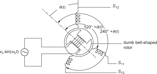
Fig. 2.20 ∣ Schematic Diagram of Synchro Transmitter

Working of Synchro Transmitter: The schematic diagram of synchro transmitter is shown in Fig. 2.20. When an AC voltage , is applied to the rotor of the synchro transmitter via slip rings as shown in Fig. 2.19 and Fig. 2.20, a magnetizing current that is induced in the rotor coil produces a sinusoidally time varying flux that is distributed in the air gap along the stator periphery that induces the voltage in each of the stator coils. The flux linking any stator coil and the induced voltage in the stator coil is proportional to the cosine of the angle between the rotor and stator coil axes as the flux in the air gap is sinusoidally distributed.

Let , and be the voltages induced in the stator coils and , and with respect to the neutral respectively. Then, when the angle between the rotor axis and stator coil S₂ is as shown in Fig. 2.20, the voltage induced in the stator coils are given by:

(2.1)

(2.2)

(2.3)

Also, the terminal voltages of the stator are given by:

(2.4)

(2.5)

(2.6)

The terminal voltages of the stator that are given in Eqs. (2.4) through (2.6) can be plotted as shown in Fig. 2.21.

Fig. 2.21 ∣ Waveform for the terminal voltages of the stator

Electrical Zero Position of Transmitter: When the rotor axis and stator coil are in parallel, i.e., when = 0, a maximum voltage will be induced in the corresponding stator coil while the terminal voltage across the other two terminals is zero. That corresponding position of the rotor is defined as the “electrical zero” position of the transmitter. For the shown rotor position in Fig. 2.19, if the angle = 0, then from Eqs. (2.1) through (2.3), it is clear that the maximum voltage is induced in the stator coil and also, the terminal voltage across the other two terminals, i.e., is zero. This electrical zero position is used as reference to specify the angular position of the rotor.

2.11.2 Synchro Control Transformer

The synchro control transformer is similar to the synchro transmitter with the exception in the shape of the rotor. The shape of the rotor in the synchro control transformer is made cylindrical to have uniform air gap. The generated emf of the synchro transmitter is applied as an input to the stator coils of the synchro control transformer. The load whose position is to be maintained at a desired value is connected with the rotor shaft. The constructional features and schematic diagram of a synchro transmitter are shown in Fig. 2.22(a) and Fig. 2.22(b) respectively.

Fig. 2.22 ∣ (a) Constructional features of Synchro control transformer

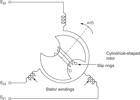
Fig. 2.22 ∣ (b) Schematic diagram of Synchro control transformer

Working of Synchro Control Transformer: The terminal voltages obtained across the stator windings of transmitter is applied across the stator windings of control transformer. Due to the presence of uniform air gap and the position of rotor, a voltage will be induced in the rotor winding. This voltage is known as error voltage that is proportional to the difference in the rotor positions of transmitter and control transformer. In addition, this induced voltage in the rotor is used to drive the motor for correcting the position of load.

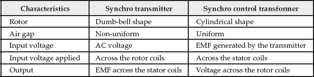
The constructional details of the synchro transmitter and the synchro control transformer are given in Table. 2.11.

Table 2.11 ∣ Synchro transmitter and synchro control transformer

2.11.3 Synchro Error Detector

The system (synchro transmitter−synchro control transformer pair) acts as an error detector. The schematic diagram of the synchro error detector is shown in Fig. 2.23.

Fig. 2.23 ∣ Synchro error detector

Let and be the angles through which the rotor of synchro transmitter and synchro control transformer rotates in the same direction. When an AC supply is applied to the rotor of the synchro transmitter an induced voltage produced in the stator will be applied to the stator of the synchro control transformer. Due to the voltage induced in the stator of control transformer, an induced voltage will be produced in the rotor of control ­transformer, which is proportional to cosine of the angle difference between the rotor positions, i.e., . The voltage induced in the rotor of the control transformer is known as error voltage and is given by

(2.7)

where the constant of proportionality K_s is called gain of the error detector.

When the error voltage is modulated and amplified, it can be used to drive the servomotor that is connected to load.

Electrical Zero Position of Synchro Control Transformer: When the two rotors are at right angles, the voltage induced in the rotor of the control transformer is zero. This position is known as the “electrical zero” position of the control transformer.

2.12 Servomotors

The servomotors are used to convert an electrical signal (control voltage) applied to them into an angular displacement of the shaft. They are normally coupled to the controlled device by a gear train or some mechanical linkage. Their ratings vary from a fractional kilowatt to few kilowatts. The main objective of the servomotor system is to control the position of an object and hence the system is known as servomechanism.

2.12.1 Classification of Servomotor

The general classification of servomotors is shown in Fig. 2.24.

Fig. 2.24 ∣ Classification of servomotor

2.12.2 Features of Servomotor

The maximum acceleration is the most important characteristics of servo motor. For control system application, there exists a variety of servomotors. But selection of a servomotor for a particular application depends on system characteristics and its operating conditions. In general, there are some features that a servomotor should have to suit for any application.

1. Relationship between the control signal and speed should be linear.
2. Speed control should have a wider range.
3. Response should be faster.
4. There should be steady-state stability.
5. Mechanical and electrical inertia should be low.
6. Mechanical characteristics should be linear throughout the speed range.

2.12.3 DC Servomotor

DC servomotor is used in applications such as machine tools and robotics, where there is an appreciable amount of shaft power is required. DC servomotors are expensive and more efficient than AC servomotors. While deriving transfer functions, the system is approximated by a linearly lumped constant parameters model by making suitable assumptions. The modes in which it could be operated are (a) field control mode and (b) armature control mode.

Transfer Function of a Field-Controlled DC Motor: In the case of field-controlled DC motor, the armature voltage and current are kept constant. The torque developed and hence the speed of the motor will be directly proportional to the field flux, generated by the field current flowing in the field winding. When the error signal is zero, there will be no field current and hence no torque is developed. The direction of rotation of the motor depends on the polarity of the field and hence on the nature of the error signal. If the field polarity is reserved, the motor will develop torque in the opposite direction. A field-controlled DC motor is shown in Fig. 2.25

Fig. 2.25 ∣ Field controlled DC motor

Let and be the resistance and inductance of the field circuit in and respectively,

be the excitation voltage/control input of the field circuit in ,

be the current flowing through the field circuit in ,

be the torque developed by the motor in N-m,

be the moment of inertia in kg-m²,

be the coefficient of friction in N-m/(rad/sec) and

be the angular displacement of motor shaft in radians.

Here, the armature current is maintained constant by applying a constant voltage source to the armature and having a very large resistance in series with armature. Although the efficiency of the field-controlled DC motor is low, it is used for speed control.

The equivalent electrical field circuit and equivalent mechanical circuit of the load are shown in Fig. 2.26 and Fig. 2.27 respectively.

Fig. 2.26 ∣ Equivalent electrical field circuit

Fig. 2.27 ∣ Equivalent mechanical circuit of load

Applying Kirchhoff's voltage law to the equivalent electrical field circuit shown in Fig. 2.26, we obtain

(2.8)

Taking Laplace transform, we obtain

(2.9)

The torque developed is proportional to the field current since the armature current is constant.

where is a constant.

Taking Laplace transform of the above equation, we obtain

(2.10)

The torque equation for the load from its equivalent mechanical circuit shown in Fig. 2.27 is given by

(2.11)

Taking Laplace transform of the above equation, we obtain

(2.12)

Comparing Eqn. (2.10) and Eqn. (2.12), we obtain

Substituting Eqn. (2.9) in the above equation, we obtain

Hence, the transfer function is given by

where , mechanical time constant and field time constant .

The resultant transfer function of field-controlled DC motor is of higher order (third order) due to the field inductance that is not negligible. Hence, the stability of the system is poor when compared to the armature-controlled DC motor.

Transfer Function of an Armature-Controlled DC Servo Motor: A DC armature controlled motor is shown in Fig. 2.28.

Fig. 2.28 ∣ Armature controlled DC motor

Let and be the resistance and inductance of the armature circuit in and respectively,

be the applied voltage in the armature circuit in ,

be the current flowing through the armature circuit in ,

be the back emf in the armature circuit in V,

be the constant field current flowing through the field windings in A,

be the torque developed in the motor in N-m,

be the moment of inertia in kg-m²,

be the coefficient of friction in N-m/(rad/sec) and

be the angular displacement of motor shaft in radians.

Control signals are applied to the armature current and the field current is maintained at a constant value. Maintaining a constant field current is easier than maintaining a constant armature current due to the presence of back emf in the armature circuit.

The equivalent electrical armature circuit and equivalent mechanical circuit of the load are shown in Fig. 2.29 and Fig. 2.30 respectively.

Fig. 2.29 ∣ Equivalent electrical armature circuit

Fig. 2.30 ∣ Equivalent mechanical circuit of load

Applying Kirchhoff's voltage law to the armature circuit shown in Fig. 2.29, we obtain

(2.13)

Taking Laplace transform of the above equation, we have

(2.14)

Since the field current is kept constant, the torque developed is proportional to the armature current. Therefore,

(2.15)

Taking Laplace transform of the above equation, we have

(2.16)

The torque equation for the load from its equivalent mechanical circuit shown in Fig. 2.30 is given by

(2.17)

Taking Laplace transform of the above equation, we have

(2.18)

Substituting Eqn. (2.16) in Eqn. (2.18), we have

Substituting Eqn. (2.14) in the above equation, we obtain

(2.19)

Motor back emf is proportional to speed and therefore,

where is the back emf constant.

Taking Laplace transform of the above equation, we have

(2.20)

Substituting Eqn. (2.20) in Eqn. (2.19), we have

Therefore, the transfer function is given by

where is the Mechanical time constant and = is the armature time constant.

Generally, for an armature controlled machine, τ_a = 0. Hence,

Advantages of DC Servomotor

The advantages of DC servomotor are:

1. It has a higher power output than a 50Hz motor of the same size and weight.
2. Linear characteristics can easily be achieved.
3. Speed control can be easily achieved (from zero speed to full speed).
4. Quick acceleration of loads is possible due to high torque to inertia ratio.
5. Time constants in the transfer function have low values.
6. It involves less acoustic noise.
7. Encoder sets resolution and accuracy.
8. It has higher efficiency since it can reach up to 90% of light loads.
9. It is free from vibration and resonance.

Disadvantages of DC Servomotor

The disadvantages of DC servomotor are:

1. It involves higher cost due to its complex architecture (encoders, servo drives).
2. It requires larger motor or gear box.
3. There is necessity of safety circuits.
4. It needs to be tuned so as to get steady feedback loop.
5. Motor generates peak power only at higher speeds and requires frequent gearing.
6. Inefficient cooling mechanism. If motors are ventilated, they get easily contaminated.

2.12.4 AC Servomotor

The AC servomotor is a two-phase induction motor with some special design features. The simple constructional feature of AC servomotor is shown in Fig. 2.31. It comprises of a stator winding and a rotor, which may take one of several forms: (i) squirrel cage, (ii) drag cup and (iii) solid iron.

Fig. 2.31 ∣ AC servomotor

The stator consists of two pole-pairs mounted on the inner periphery of the stator, such that their axes are at an angle of in space. The rotor bars are placed on the slots and short-circuited at both ends by end rings. The diameter of the rotor is kept small in order to reduce inertia and to obtain good accelerating characteristics.

Each pole-pair carries a winding. The exciting current in the windings should have a phase displacement of as shown in Fig. 2.32. The voltages applied to these windings are not balanced.

Fig. 2.32 ∣ Exciting currents in the winding

Under normal operating conditions, a fixed voltage form a constant voltage source is applied to one phase, which is called the reference phase. The other phase called the control phase is energized by a voltage of variable magnitude and polarity, which is at out of phase with respect to the fixed phase. The control phase is usually applied from a servo amplifier. The direction of rotation reverses if the phase sequence is reversed.

In feedback control system, the AC servomotor resembles two-phase induction motor. The differences that exist between normal induction motor and servomotor are:

1. To achieve linear speed torque characteristics, the rotor resistance of the servomotor is made high so that the ratio X/R is made small.
2. Phase difference between the excitation voltages applied to two stator windings is 90°.

The torque-speed characteristics for the induction motor and servomotor are shown in Fig. 2.33.

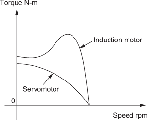
Fig. 2.33 ∣ Torque-speed characteristics

In the two-phase servomotor, the polarity of the control voltage determines the direction of rotation. Then the instantaneous control voltage is of the form

sin  for

sin  for

Since the reference voltage is constant, the torque and the angular speed are also functions of the control voltage . If variations in are also compared with the ac supply frequency, the torque developed by the motor is proportional to . Figure 2.34 shows the curves versus t, versus t and torque versus t. The angular speed at steady state is proportional to the control voltage .

Transfer Function of AC Servomotor: For higher values of rotor resistance, the torque−speed characteristics are linear. For servo application, the motor characteristics should be linear with negative slope. Therefore, ordinary two-phase induction motor with low rotor resistance is not suitable for servo applications. Figure 2.35 shows the speed−torque characteristics of servomotor for different values of control voltage.

Fig. 2.34 ∣ , and θ versus time

Fig. 2.35 ∣ Torque − speed characteristics

The following assumptions are to be made to derive the transfer function of the motor:

1. Linear portion of the torque−speed curve is extended up to the high-speed region since the servomotor operates normally at high speed.
2. Speed−torque characteristics for different voltages are assumed as straight line parallel to the characteristics at rated control voltage.

The blocked rotor torque at rated voltage per unit control voltage is represented as follows:

The slope of the linearized torque−speed curve is given by

Then for any torque , the family of straight line torque−speed curve is represented as follows:

If we consider that the moment of inertia of the motor and shaft is and the viscous friction is , we have

Taking the Laplace transform, we obtain

Therefore, the transfer function of the two-phase motor is obtained as

or

where is the motor gain constant and is the motor time constant.

Advantages of AC Servomotors

1. AC servomotors involve low cost and low maintenance since there is no commutator and brushes.
2. These are of high efficiency.

Applications of AC Servomotors

1. These are used in X−Y recorders.
2. These are also used in disk drives, tape drives printers, etc.

2.12.5 Comparison between AC Servomotor and DC Servomotor

The comparison between the AC servomotor and DC servomotor based on different characteristics is given in Table 2.12.

Table 2.12 ∣ Comparison between AC and DC servomotors

2.13 Tachogenerators

Tachogenerator is an electromechanical device that converts mechanical energy (shaft speed) to a proportional electrical energy (voltage). It is an ordinary generator that generates a voltage proportional to the magnitude of the angular velocity of the shaft. It is used as speed indicator, velocity feedback device and signal integrator. Tachogenerators are classified as AC tachogenerator and DC tachogenerator.

2.13.1 DC Tachogenerator

The schematic representation of a DC tachogenerator is shown in Fig. 2.36. The iron core rotor is the most common part in all DC tachogenerator. A DC tachogenerator is an ordinary DC generator with linear characteristics. The parts of the DC tachogenerator are stator with a permanent magnet to produce necessary magnetic field, rotating armature circuit connected to the commutator and brush assembly. The output voltage is measured across the pair of brushes that are connected with commutators. If required, modulated output of DC tachogenerator can be used in controlling the AC system components.

The output voltage of the tachogenerator is proportional to the angular velocity of the shaft. The polarity of the output voltage depends on the direction of rotation of the shaft.

Fig. 2.36 ∣ Schematic diagram of DC Tachogenerator

Let be the output voltage of tachogenerator in volts,

be the angular displacements in rad,

be the angular velocity in rad/sec and

be the sensitivity of tachogenerator in volts−sec/rad.

The output voltage of tachogenerator,

or,

Taking Laplace transform of the above equation, we obtain

Hence, the transfer function of DC tachogenerator is

Advantages of DC Tachogenerator

The advantages of DC tachogenerator are:

1. It is used alongwith high pass output filters to reduce the servo velocity lags.
2. It generates very high-voltage gradients in small sizes.
3. There is no presence of residual voltage at zero speed.

Disadvantages of DC Tachogenerator

The disadvantages of DC tachogenerator are:

1. inherent ripples in the output waveform
2. poor commutation
3. requirement of additional filter to avoid the interference

2.13.2 AC Tachogenerator

The AC tachogenerator and a two-phase induction motor resemble each other. The parts of the AC tachogenerator are two-stator windings (reference and quadrature windings) with the angle between their axes as 90° are fixed on the inner periphery of stator arranged in space quadrature and the squirrel cage rotor. Stator windings are referred to as reference winding and output winding. The reference winding is excited by a sinusoidal voltage with frequency, . When the rotor rotates, a voltage will be induced in the quadrature winding. The schematic diagram of AC tachogenerator is shown in Fig. 2.37. An AC tachogenerator alongwith a phase-sensitive demodulator circuit can be used in control system to convert an AC output to a DC output.

If the reference winding is excited by the voltage , a reference flux will be produced in the reference winding due to the presence of negligible resistance and reactance in the reference coil. The rotor speed equation is given by

Fig. 2.37 ∣ Schematic diagram of AC Tachogenerator

The induced voltage produced in the quadrature winding, which is in phase with the voltage applied in the reference coil, is directly proportional to the rotor speed. The modulated signal available at the output terminal is given by

Taking Laplace transform, we obtain

The above equation gives the transfer function of the AC tachogenerator, which is same as the transfer function of DC tachogenerator.

2.14 Stepper Motor

A special type of synchronous motor designed to rotate through a specific angle for each electrical pulse applied is known as stepper motor. The specific angle through which the stepper motor rotates is called step. Electrical pulses are received from the control unit of stepper motor. Stepper motor is used alongwith electronic switching devices whose function is to switch the control windings of stepper motor according to the command received.

The stepper motor has gained importance in recent years because of the ease with which it can be interfaced with digital circuits. The stepper motor completes a full rotation by sequencing through a series of discrete rotational steps (stepwise rotation). Each step position is an equilibrium position, so that without further excitation the rotor position stays at the latest step. Thus, continuous rotation is achieved by a train of input pulses, each of which causes an advance of one step. The stepper motor can be variable reluctance, permanent magnet or hybrid stepper motor depending on the type of rotor. The stepper motor can also be classified into two-phase, three-phase or four-phase stepper motor depending on the number of windings on the stator.

2.14.1 Permanent Magnet Stepper Motor

In this type of stepper motor, the stator has salient poles that carry control windings. A phase is created when the two control windings are connected in series. The rotor of this type of stepper motor is made in the form of a spider cast integral permanent magnet or assembled permanent magnets. The schematic diagram showing the different types of rotor structure is shown in Fig. 2.38.

Fig. 2.38 ∣ Rotor structure types

The permanent magnet stepper motor operates at a larger steps upto 90° at a maximum response rate of 300 pps.

2.14.2 Variable Reluctance Stepper Motor

In this type of stepper motor, it has a single or several stacks of stator and rotor. The stator has a common frame, whereas the rotor has a common shaft. The stator and rotor of this type of stepper motor has toothed structure. The longitudinal cross sectional view of three-stack variable reluctance stepper motor is shown in Fig. 2.39.

Fig. 2.39 ∣ 3 Stack variable reluctance motor

The difference in angular displacement of stator and rotor when the teeth of the rotors are perfectly aligned is given by

where n is the number of stacks and T is the number of rotor teeth.

The schematic diagram explaining the concept of the separation between the stator and rotor is shown in Fig. 2.40.

Fig. 2.40 ∣ Separation between stator and rotor

2.14.3 Hybrid Stepper Motor

This is similar to the permanent magnet stepper motor with the constructional features rotor adopted from variable reluctance stepper motor. The polarities of the teeth on the stack of the rotor at both the ends are of different polarities. Thus, the two sets of teeth in the rotor are displaced from each other by one-half of the tooth pitch (pole pitch). The constructional features of this type of stepper motor are shown in Fig. 2.41(a) and (b).

Fig. 2.41 ∣ Constructional features of hybrid stepper motor

2.14.4 Operation of Stepper Motor

Depending on the step angle by which the stepper motor rotates, the operation of stepper motor can be classified as

1. full-step operation
2. half-step operation
3. micro-step operation

Full-Step Operation: In this type of operation, the stepper motor moves one full step for each of the input pulse applied.

Full step =

where is the number of rotor poles and the number of stator pole pairs.

Half Step Operation: In this type of operation, the stepper motor moves one-half of the full step for each of the input pulse applied. If in the full-step operation of stepper motor, for each input pulse the motor rotates at , then in the half-step operation of stepper motor, the motor will rotate at for each input pulse.

Micro Step Operation: In this type of operation, the stepper motor moves through an angle of 1/10, 1/16, 1/32 and 1/125 of a full step. The major advantage of this type of operation is that it provides much finer resolution.

2.14.5 Advantages of Stepper Motor

The advantages of stepper motor are:

1. It is compatible with digital systems.
2. No sensors are required to sense the speed and position.
3. Motors are available in larger power ratings with reduced cost.
4. Motors are available with the torque range of 0.5 micro N-m to 100 N-m.
5. It is used to upgrade mechanical systems to give greater precision and production rate.

2.14.6 Applications of Stepper Motor

The applications of stepper motor are:

1. It is used in computer peripherals (printers, disk drives, etc.), X–Y plotters, scientific instruments and machine tools.
2. It is used in quartz crystal watches.
3. Many supporting roles in the manufacture of packaged foodstuffs, commercial end products and even in the production of science fiction movies.

2.15 Gear Trains

The conventional servomotor usually operates at high speeds with low torque. Gear trains are used in servo positioning applications to operate the servomotor at low speed with low torque. In addition, to alter the speed-to-torque ratio of the rotational power transmitted from motor-to-load gear trains are used. Gear trains are necessary to match the torque requirement of the load to that of the motor. Hence, the knowledge of the actions of a gear train is important to the control systems designer. The analogous component of gear train in mechanical rotational system is the transformer in electrical system that is shown in Fig. 2.42 and Fig. 2.43.

Fig. 2.42 ∣ Schematic diagram of gear trains

Fig. 2.43 ∣ Equivalent circuit of gear trains

2.15.1 Single Gear Train

The schematic diagram representing the gear train driving the load is shown in Fig. 2.44. The gear train shown in Fig. 2.44 consists of two gears with teeth N_M and N_L.The gear 1 (primary gear) is connected to motor shaft and gear 2 (secondary gear) is connected to load shaft. The subscript in the following section denotes the gear 1 (primary gear) and subscript in the following section denotes the gear 2 (secondary gear).

Let and be the number of teeth's in gears,

and be the radius of gears,

and be the angular displacement of shafts,

and be the moment of inertia,

and be the viscous friction coefficient,

be the load torque developed by motor,

be the torque developed by motor,

be the torque transmitted to gear 2 from gear 1 and

be the load torque.

Fig. 2.44 ∣ Schematic diagram for gear trains

The torque developed by motor is balanced by the sum of load torque requirement on gear 1 and opposing torque due to and . Hence, the torque balance equation for motor shaft is given by

(2.21)

The torque transmitted to gear 2 is balanced by the sum of load torque and opposing torque balance equation for load shaft is given by

(2.22)

When the motor drives the load, the linear distance travelled by each gear is same. The linear distance travelled by a gear is given by the product of the radius and angular displacement.

Linear distance travelled by the gear

Therefore, (2.23)

The number of teeth in each gear is proportional to its radius.

Therefore, and

Hence, (2.24)

From Eqn. (2.23) and Eqn. (2.24), we obtain

(2.25)

In ideal gear train system, there is no power loss in transmission. Hence, the work done by both gears are equal. The work done by a gear is given by the product of torque acting on it and its angular displacement.

Work done by the gear (2.26)

Therefore,

(2.27)

Cross-multiplying and differentiating the above equation, we obtain

(2.28)

Therefore,

and

(2.29)

When and are angular speeds of motor shaft and load shaft respectively. ­Differentiating Eqn. (2.28) again, we obtain

Therefore,

and

(2.30)

where and are angular acceleration of motor shaft and load shaft respectively.

From Eqs. (2.23), (2.24), (2.27), (2.29) and (2.30), we obtain

(2.31)

Using the above equation, it can be said that

When the gear train increases the speed and reduces the torque.

When there is no change in speed and torque.

When the gear train decrease the speed and increase the torque.

Torque Equation Referred to Motor Shaft: In systems with gear trains, it will be easier for analysis if the torques acting on the system is transferred to one of the sides.

Equation (2.31) can be rewritten as follows:

  (2.32)

  (2.33)

(2.34)

Substituting the values for from the above equations in Eqn. (2.22), we obtain

Multiplying the above equation by , we obtain

(2.35)

Substituting the value for from Eqn. (2.35) in Eqn. (2.21), we obtain

(2.36)

where total equivalent moment of inertia referred to motor shaft

and total equivalent viscous friction coefficient referred to motor shaft.

Equation (2.36) is the torque equation of the gear train system referred to motor shaft.

Torque Equation Referred to Load Shaft:

From Eqn. (2.31), we can write

  (2.37)

  (2.38)

(2.39)

Substituting the values of from the above equations in Eqn. (2.21), we obtain

(2.40)

Substituting the value of from Eqn. (2.22) in Eqn. (2.40), we obtain

Multiplying the above equation by , we obtain

(2.41)

where total equivalent moment of inertia referred to load shaft and Total equivalent viscous friction coefficient referred to load shaft.

Equation (2.41) is the torque equation of gear train systems referred to load shaft.

2.15.2 Multiple Gear Trains

The concept of equivalent inertia, friction and torque just described can also be extended to a multiple gear train system as shown in Fig. 2.45.

Fig. 2.45 ∣ Multiple gear train system

The inertia and at the load shaft are referred to shaft 2 and the equivalent quantities are as follows:

The equivalent inertia and friction at shaft 2 are now referred to shaft 1 resulting

Similarly, the inertia and friction at shaft 1 can be referred to the load shaft. Therefore, we have

It is noted that direction of each gear is opposite to the direction of previous gear in the given gear train system.

Fig. E2.10 ∣ A simple gear system

Solution: Using Eqn. 2.31, we obtain the gear ratio as

For the given gear system, the subscripts M and L in the above equation can be changed into 1 and 2 respectively. Hence, the above equation can be modified as

where and are number of turns in the gear 1and gear 2 respectively.

and are the radius of gear 1 and gear 2 respectively in .

and are the torques of gear 1 and gear 2 respectively in .

and are the angular displacements of gear 1 and gear 2 respectively in .

and are the angular velocities of gear 1 and gear 2 respectively in .

and are the angular accelerations of gear 1 and gear 2 respectively in .

From the given data, we have

1. Ratio of diameters of gears

   Using the above equation, we obtain

   

   

2. Angular displacement of gear 2

   Using the above equation, we obtain

   

   

3. Angular velocity of gear 2

   Using the above equation, we obtain

   

   

4. Angular acceleration of gear 1

   Using the above equation, we obtain

   

   

5. Torque of gear 2

   Using the above equation, we obtain

   

   

Review Questions

1. What do you mean by an electromechanical system and why is it required?
2. What are the subsystems available under electromechanical systems?
3. What are the different laws used for governing an electromechanical system?
4. Explain hydraulic systems.
5. What are the advantages and disadvantages of hydraulic systems?
6. What are devices used in the hydraulic system?
7. Name some of the applications of hydraulic systems.
8. Explain pneumatic systems.
9. What are the basic elements of the pneumatic systems? Explain.
10. What are the advantages and disadvantages of pneumatic systems?
11. What are devices used in the pneumatic system?
12. Compare pneumatic systems with hydraulic systems.
13. Explain thermal systems.
14. What are the different ways by which a heat flows from one substance to another ­substance? Explain.
15. Explain the basic elements of thermal systems.
16. What do you mean by liquid-level system?
17. What are the basic elements of liquid-level system. Explain.
18. Tabulate the analogous quantities of different physical systems (hydraulic, thermal, ­pneumatic and liquid-level systems) with electrical systems.
19. With a neat block diagram, explain the control system components.
20. Explain the following terms:
    1. Controller output as a percentage value
    2. Measured value as a percentage value
    3. Set point as a percentage value
    4. Error as a percentage value
21. What are the general classifications of a controller?
22. List the types of analog controllers.
23. Explain the digital controller with a neat block diagram.
24. With a neat block diagram, explain the fuzzy controller.
25. What are the advantages of digital controller?
26. Define electronic controllers.
27. How is the controller classified based on the control action performed by it?
28. Define ON–OFF controller.
29. Explain the different types of ON–OFF controller.
30. What do you mean by neutral zone in the ON–OFF controller?
31. Draw the electronic version of two position ON–OFF controller.
32. What are the applications of two position ON–OFF controller?
33. Draw the electronic version of three position ON–OFF controller.
34. With a neat block diagram, explain the proportional controller or P-controller.
35. Define proportional band of P-controller.
36. Explain the electronic P-controller using inverting and non-inverting amplifier.
37. What are the advantages and disadvantages of P-controller?
38. With a neat block diagram, explain the following controllers:
    1. Integral controller or I-controller
    2. Derivative controller or D-controller
    3. Proportional−integral controller or PI-controller
    4. Proportional−derivative controller or PD-controller
    5. Proportional−integral−derivative controller or PID-controller.
39. Explain the following electronic controllers:
    1. I-controller using inverting amplifier
    2. D-controller using inverting amplifier
    3. PI-controller using inverting amplifier
    4. PD-controller using inverting amplifier
    5. PID controller using inverting amplifier
40. What are the advantages and disadvantages of the following controllers?
    1. I-controller
    2. D-controller
    3. PI-controller
    4. PD-controller
    5. PID-controller
41. With a neat diagram, explain DC and AC potentiometer.
42. What are the characteristics of potentiometers?
43. Define power-handling capacity in potentiometer.
44. What are the applications of potentiometers?
45. Explain the concept of synchro.
46. Differentiate the characteristics of synchro transmitter and synchro control transformer.
47. With a neat diagram, explain synchro transmitter.
48. Explain synchro control transformer with a neat diagram.
49. Define electrical zero position of synchro control transformer and synchro transmitter.
50. Explain the application of synchro as synchro error detector.
51. Explain the concept, classification and features of servomotor.
52. Derive the transfer function of field- and armature-controlled DC motor.
53. What are the advantages and disadvantages of DC servomotor?
54. Explain the concept of AC servomotor and derive its transfer function.
55. Compare different characteristics of AC servomotor and DC servomotor.
56. Define tachogenerator. What are the different types of tachogenerator?
57. Derive the transfer function of DC tachogenerator. Also, mention its advantages and ­disadvantages.
58. Explain the concept of AC tachogenerator.
59. Explain the concept of stepper motor. Also, explain briefly about the different types of stepper motor.
60. Explain the different concepts of stepper motor operation.
61. What are the advantages and applications of stepper motor.
62. Explain gear train.
63. With a neat schematic diagram, explain the concept of single gear train and derive all the possible relations.
64. With a neat schematic diagram, explain the concept of multiple gear trains.
65. Consider two identical dashpots connected in series as shown in Fig. Q2.65. Obtain the transfer functions of the system.
    

    Fig. Q2.65

66. The pneumatic system in Fig. Q2.66 has two identical bellows. The outputs of the bellows (mechanical ends) are connected by a link from which the mechanical linear movement is taken. The linear movement is proportional to the differential force of the bellows. The linear movement is zero if there exists a steady input pressure. Determine (i) the transfer function of the given system relating the input pressure to linear displacement output if the bellows stiffness is and (ii) determine the steady-state value of for a unit step change in input pressure.
    

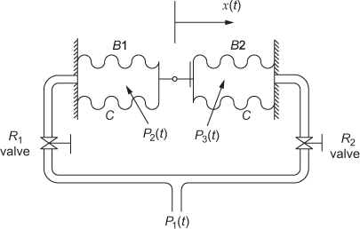
    Fig. Q2.66

67. For the non-interacting liquid-level system shown in Fig. Q2.67, determine the transfer function of the system relating the inflow rate into the tank 1 and the liquid level in the tank 2.
    

    Fig. Q2.67

68. For the interacting liquid-level system shown in Fig. Q2.68(a), determine the transfer function of the system relating (i) the inflow rate and the height of liquid in tank 2 , (ii) the inflow rate and the outflow rate and (iii) the inflow rate and the height of liquid in tank 1 when the inflow of liquid is at (a) first tank and (b) second tank.
    

    Fig. Q2.68

69. The composite gear system that consists of many gears is shown in Fig. Q2.69. Obtain the (i) angular displacement of gear 4 and gear 6 if the angular displacement of gear 2 is 10 , (ii) angular velocity of gear 1 and gear 2 if the angular velocity of gear 6 is 15 and (iii) torque of gear 3 and gear 7 if the torque of gear 1 is 20 N-m
    

    Fig. Q2.69