12

PHYSIOLOGICAL CONTROL SYSTEMS

12.1 Introduction

Physiological and Engineering control system look similar to each other. A physiological control system explores some control problem related to biological ­environment and provides solution to the control researchers. The involvement of control theory makes the biomedical application more efficient and natural. The control mechanism in the biomedical application that comprises components that are necessary for maintenance of homeostasis at all levels of living systems is discussed in this chapter. The positive and negative feedback control mechanisms for maintaining homeostasis are also discussed.

12.2 Physiological Control Systems

The collection of trillions of cells composes the human body functions in a pattern that is essential for continuation of life process. In physiological control system the human body is considered as a system and the internal environment of the human body refers to each and everything present within the body where the cells live and work together. A specific ­optimum condition should be maintained within the body for proper functioning of cells which in turn makes the tissues, organs and the total system work properly. It is also necessary that the composition and fluid temperature around the cells must be constant for the cells to survive and function properly.

Homeostasis is the property of a system that helps in maintaining the consistency of the internal environment of the system. In addition, homeostasis can be defined as the property in which the variables of the system are regulated for maintaining a stable and relatively constant environment in the internal ­environment of the system despite the changes in the external environment. At the optimal temperature, when the internal environment of a system has optimal concentration of gases, nutrients, ions and water, the system is in homeostasis condition. The relationship between the human body and homeostasis is shown in Fig. 12.1. The human body will be operated in such a way that the homeostasis is maintained and it is essential for the survival.

Fig. 12.1 ∣ Relationship between human body and homeostasis

12.3 Properties of Physiological Control Systems

The properties of physiological control systems are:

1. Physiological control system is corrected in such a way that the stability of the system is maintained.
2. Delay exists in correction of error sensed by a system.
3. The correction made by a system is proportional to the error.
4. Residual error exists even after the correction.
5. The gain of a system is used for assessing the effectiveness of that system.

The characteristic curve of a physiological control system that depicts the properties of the system is shown in Fig. 12.2.

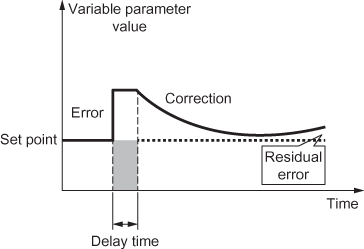
Fig. 12.2 ∣ Characteristic curve of a control system

The special properties of a physiological control system are:

1. A system has a variable gain that is used to control the oscillatory changes.
2. A system has a variable set point as the optimal value of a parameter varies for ­different conditions.
3. In certain conditions, a system anticipates the error and takes necessary action.
4. In a system, two or more control mechanisms are linked together for controlling a variable.

12.3.1 Target of the Homeostasis

The different systems in the human body—digestive system, circulatory system, respiratory system, excretory system, nervous system, endocrine system, immune system, musculo­skeletal system and integumentary system—help in their own way for maintaining the homeostasis in the internal environment. Therefore, the following points are the collective target of the human body or homeostasis:

1. Maintaining adequate concentration of energy sources
2. Having adequate and continuous supply of oxidants
3. Limiting the concentration of waste materials
4. Sustaining optimum value of pH for proper functioning
5. Maintaining concentration of water, salt and electrolytes in the system
6. Regulation of volume, pressure and temperature of the body within the sustainable range

12.3.2 Imbalance in the Homeostasis

All the organs present within a body act together through a combination of hormonal and nervous mechanisms for maintaining the homeostasis in the internal environment of the body. In day-to-day activities, the functions such as regulation of respiratory gases, ­protection against disease agents (pathogens), fluid and salt balance maintenance, regulation of energy and nutrient supply and maintenance of constant body temperature are regulated by the human body. In addition, when the human body gets injured, it must have the capability to repair itself. The following reasons cause an imbalance in the homeostasis:

1. Due to external disturbance, the property of homeostasis gets disturbed and may cause diseases in the body.
2. Due to reduction in the efficiency of the system as the organism ages.
3. Resultant of unstable internal environment in the system due to reduction of efficiency which increases the risk of illness.
4. Physical changes associated with aging.

Some examples of homeostatic imbalances are high core temperature, increase in concentration of salt in the blood or decrease in concentration of oxygen which generate sensations such as warmth, thirst or breathlessness.

12.3.3 Homeostasis Control Mechanisms

The control mechanism used for maintaining the consistency of the internal environment is called homeostasis control mechanism. The homeostasis control mechanism is designed to re-establish homeostasis when there is an imbalance in the internal environment due to improper functioning of cells or due to ­external environment disturbances. The behaviour such as removal of sweater, drinking of water or slowing down the biological process will result in restoration of homeostatic imbalances that are listed in the previous section.

The homeostatic control mechanism should have at least three parts for restoring the homeostasis imbalances. The simple homeostatic control mechanism is shown in Fig. 12.3.

Fig. 12.3 ∣ Homeostatic control mechanism

The three major parts that are available in the control mechanism as shown in Fig. 12.3 alongwith the functions are listed below:

1. Receptor: It is a sensing component that monitors and responds to changes in the environment and sends a stimulus to the control centre.
2. Control centre: It receives the information from receptor and sets the range at which a variable is maintained and sends an appropriate response for the stimulus to the effector.
3. Effector: It receives the signal from the control centre and corrects the homeostasis imbalances.

The homeostatic control mechanism can be clearly understood with the help of an ­example. If the human body (system) senses hyperglycaemia, i.e., high blood sugar level, it is a homeostasis imbalance and the control mechanism must take necessary actions to balance the blood sugar level. The three major parts required for correcting this imbalance are listed below alongwith their functions.

1. Pancreas and beta cells—Sensor and control centre: It determines the sugar level and secretes insulin, i.e., stimulus to the blood.
2. Liver and Muscle cells—Effector: Liver takes glucose from the blood, converts to ­glycogen and stores it. Muscle cells use this glycogen for contraction. Hence, the blood glucose level gets reduced.

For the above example, sensor and control centre are the same. Hence, only two parts exist in the control mechanism for maintaining the blood sugar level, i.e., homeostasis imbalance.

12.4 Block Diagram of the Physiological Control System

The block diagram representing a typical physiological control system is shown in Fig. 12.4.

Fig. 12.4 ∣ Block diagram of physiological control system

The set point is the pre-defined and pre-set value and the optimum value of a ­parameter. The sensor continuously monitors the value of the parameter and sends the real-time value to the control centre. The control centre compares the real time and pre-defined value of the parameter and generates an error signal and in turn generates a response signal, i.e., ­stimulus. Finally, the effector takes the signal generated from the control centre and makes the parameter value to be maintained at a pre-defined value. The example discussed in Section 12.3.3 can be represented in the form of a block diagram as shown in Fig. 12.5.

Fig. 12.5 ∣ Physiological control system for maintaining blood sugar level

Any physical system has the natural tendency towards disorderliness and the control mechanism should work in such a way that the orderliness is maintained. Although the physio­logical control system performs to maintain the constancy of the homeostasis, the main objective is to achieve the steady-state value. The three methods by which the steady state can be achieved are feedback, hierarchical communication and adaptation.

If the external disturbances exist in the physiological control system, then it is called ­extrinsic; otherwise, it is called intrinsic. If the homeostatic control mechanism fails to restore the homeostasis imbalance in the internal environment when the external ­disturbance is high, then the living organism will engage in a behaviour such that the homeostasis ­imbalance is rectified.

12.4.1 Types of Control Mechanism

The control mechanism can be classified into different types based on the feedback ­mechanism. The two different types of feedback mechanism are positive feedback ­mechanism and ­negative feedback mechanism. The detailed description of these two types of ­mechanism alongwith their advantages and disadvantages is discussed here. In a ­positive feedback ­control mechanism, the set point and output values are added. In a negative ­feedback ­control mechanism, the set point and output values are subtracted.

Positive feedback mechanism

The positive feedback control mechanism is used by a very few organs in the system. Mostly, this is used for intensifying a change instead of correcting it. In positive feedback ­mechanism, the system acts in such a way that the imbalance or the perturbation increases. In addition, the positive feedback mechanism leads to a vicious cycle, i.e., when A produces more of B, B produces more of A. Further, the positive feedback mechanism acts in such a way that the stimulus gets intensified. In some cases, it is necessary to increase the stimulus. The ­general block diagram of positive feedback control mechanism is shown in Fig. 12.6.

Fig. 12.6 ∣ Positive feedback control system

The example of positive feedback mechanism is shown in Fig. 12.7, which regulates the child birth.

Fig. 12.7 ∣ Positive feedback mechanism

Also, examples for the positive feedback mechanism that leads to harmful effects are shown below:

1. When the homeostasis imbalance causes fever, a positive feedback in the control mechanism may increase the body temperature continuously. The continuous increase in temperature increases cellular proteins that cause metabolism to stop and results in death.
2. When the homeostasis imbalance called chronic hypertension exists in the system, it can favour the atherosclerosis process that causes the lumen of blood vessels to ­narrow. Then, it intensifies the hypertension and brings on more damage to the walls of blood vessels.

Negative feedback mechanism

The negative feedback mechanism is used in the system for reducing the homeostatic imbalance. Mostly, this is used for making the system self-regulatory so that the stability of the system can be achieved by reducing the effect of fluctuations. In negative feedback mechanism, right amount of corrective measure is applied in the most timely manner, which can make the system very stable, accurate and responsive. The general block diagram of negative feedback control mechanism is shown in Fig. 12.8.

Fig. 12.8 ∣ Negative feedback control system

The simplest and most fundamental of the physiological control system is the muscle stretch reflex. The knee jerk reflex, an example of muscle stretch reflex is used as a routine medical examination in assessing the state of the nervous system. When a sharp tap is given to the patellar tendon in the knee, it leads to an abrupt stretching of the thigh muscle to which patellar tendon is attached. The muscle spindles called stretch receptors get activated due to the stretch in the thigh muscle. The information about the magnitude of the stretch gets encoded by the neural impulses and is sent to the spinal cord of the system through the ­afferent nerve fibers. The different motor neurons connected to different afferent nerves get activated. This sends the efferent neural impulses back to the same thigh ­muscle that ­produces a contraction of the muscle and hence results in extension of knee joint. This ­concept of reflex is shown in Fig. 12.9.

Fig. 12.9 ∣ Concept of reflex

The block diagram representing this type of reflex is shown in Fig. 12.10. In this example, the thigh muscle corresponds to the plant or controlled system. The initial stretch produced by taping the knee is known as disturbance . The input of the feedback sensor will be the amount of stretch , which is produced in proportion to the . The feedback sensor, i.e., muscle spindle, translates into an increase in afferent neural signal sent to the reflex centre or the controller. The reflex centre in this system will be the spinal cord. The output of the controller will increase the efferent neural signal , which is directed back to the thigh muscle. This is an example of negative feedback system, since the initial ­tap-induced disturbance leads to a controller action that reduces the effect of the disturbance.

Fig. 12.10 ∣ Block diagram representation of the muscle stretch reflex

Some more examples of negative feedback mechanism are:

1. When the body senses increased temperature in the surrounding, the thermoregulatory centre in the brain situated in hypothalamus makes the sweat glands on the skin to secrete sweat. This causes the body to lose heat and maintain homeostasis. On the other hand, if the body senses cold temperature; then the thermoregulatory centre causes the body to shiver and thus increases the body temperature. This causes the body to ­generate more heat and maintain homeostasis by negative feedback ­mechanism.
2. When there is increase in blood pressure, there are certain sensors called baro-­receptors in the carotid arteries which sense this increase. This information is ­carried to the centres in medulla oblongata of brain stem. The response is in the form of ­vasodilatation in the peripheral blood vessels which reduces the ­peripheral ­resistance. The result is that the blood pressure is reduced and homeostasis is ­maintained.

Advantages

The advantages of negative feedback mechanism are:

1. The negative feedback mechanism is more stable than positive feedback mechanism.
2. Most useful control type since it helps in reaching the equilibrium state, whereas positive feedback can lead a system away from an equilibrium, which makes the system unstable.

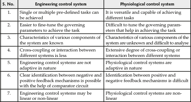
12.5 Differences Between Engineering and Physiological Control Systems

The differences between engineering and physiological control systems are given in Table 12.1.

Table 12.1 ∣ Comparison of engineering control system with physiological control system

12.6 System Elements

The different system elements are resistance capacitance and inductance. The definitions of these elements are obtained with the help of electrical circuits and then analogous to ­different systems are discussed.

12.6.1 Resistance

The Ohm's law used for determining the electrical resistance R is given by

(12.1)

where V is the voltage or driving potential across the resistor and I represents the current flowing through it. In physiological control system, V is taken as the “through” variable, called a measure of “effort” and denoted by and I is taken as the “through” variable, called a measure of “flow” and denoted by .

Therefore, in physiological control system, resistance is obtained as:

(12.2)

12.6.2 Capacitance

In electrical system, the generalized system property for storage is taken in the form of capacitance, which is defined as the amount of electrical charge (q) stored in the capacitor per unit voltage (V). Here, the relation between voltage and current is given by

(12.3)

Thus, in physiological control system, we obtain

(12.4)

12.6.3 Inductance

The final property of electrical system that stores kinetic energy is inductance. The relation between the voltage and current relating the inductance is given by

(12.5)

Thus, in physiological control system, we obtain

(12.6)

The analogous of physiological system with other systems such as electrical, mechanical, fluid, thermal and chemical are shown in Table 12.2.

Table 12.2 ∣ Analogy of variables in physiological system with other systems

12.7 Properties Related to Elements

The Kirchoff's voltage law and current law govern the electrical system. Therefore, by applying Kirchoff's voltage law for physiological system shown in Fig. 12.11, we obtain

() + () + () = 0(12.8)

Similarly, applying Kirchoff's current law for physiological system shown in Fig. 12.11, we obtain

(12.9)

Fig. 12.11 ∣ Generalized system elements network model

The elements connected in series: The resultant or equivalent value of the elements connected in series is calculated similar to the calculation used in electrical system.

Resistors in series: When the resistors are connected in series as shown in Fig. 12.12(a), the equivalent resistance is the summation of individual resistance values, i.e.,

Capacitors in series: When the capacitors are connected in series as shown in Fig. 12.12(b), the equivalent capacitance is calculated as:

The elements connected in parallel: The equivalent value of the elements connected in parallel are calculated similar to the calculation used in electrical system.

Resistors in parallel: When the resistors are connected in parallel as shown in Fig. 12.12(c), the equivalent resistance is calculated as:

Capacitors in parallel: When the capacitors are connected in parallel as shown in Fig. 12.12(d), the equivalent capacitance is determined as the summation of individual capacitance values, i.e.,

Fig. 12.12 ∣ Model properties of system elements in physiological system: (a) resistors connected in series, (b) capacitors connected in series, (c) resistors connected in parallel and (d) capacitors ­connected in parallel

12.8 Linear Models of Physiological Systems: Two ­Examples

The mathematical models are derived in this section, which characterize the input–output properties of two simple physiological models: lung mechanism and skeletal muscle.

12.8.1 Lung Mechanism

The working of lung mechanism should be studied before deriving the mathematical model of the system. The process of modelling the lung mechanism is explained below.

Airways are divided into two categories: the larger or central airways and the smaller or peripheral airways. The fluid mechanical resistances of the two categories of airways are and respectively. The chest wall cavity gets expanded by the volume of air entering the alveoli. The chest wall gets expanded by the same amount of air entering the lungs. This relation is given by the series connection of lung and chest wall compliances represented by and respectively. However, due to the presence of compliance of central airways and gas compressibility, a small fraction of volume of air is shunted away from the alveoli ­represented by shunt compliance, . In normal circumstances, this shunted volume is very small and if is increased or if or is decreased, it may lead to disease. This effect is taken into consideration by placing in parallel with and . The lung model developed with the help of these variables is shown in Fig. 12.13.

Let the pressures developed at different points of lung model shown in Fig. 12.13 be at the airway opening, at the central airways, in the alveoli and in the pleural space. The reference pressure or the ambient pressure is taken as which can be set to zero. If the flow rate of air entering the respiratory system is Q, the flow delivered to alveoli is , then the flow shunted away from alveoli be and also a mathematical relationship between and Q can be derived by as follows:

Using Kirchhoff's law to the circuit shown in Fig. 12.13,

(12.10)

and

(12.11)

Fig. 12.13 ∣ Linear model of respiratory mechanics

Differentiating Eqn. (12.10) with respect to , we obtain

Rearranging the above equation, we obtain

Substituting in the above equation, we obtain

(12.12)

Differentiating Eqn. (12.11) with respect to , we obtain

(12.13)

Differentiating Eqn. (12.13) with respect to , we obtain

(12.14)

Using Eqn. (12.12), we get

(12.15)

Substituting Eqn. (12.15) in Eqn. (12.14), we obtain

(12.16)

Using Eqn. (12.13), we obtain

(12.17)

Substituting Eqn. (12.17) in Eqn. (12.16), we obtain

Solving the above equation, we obtain

(12.18)

where

The model of the lung mechanism is represented by Eqn. (12.18).

12.8.2 Skeletal Muscle

The linearized physiological model of skeletal muscle in the human body is shown in Fig. 12.14.

Fig. 12.14 ∣ Model of a skeletal muscle

Let and represent the force developed by the active contractile element of the muscle and actual force developed due to mechanical properties of muscle respectively. The ­viscous damping inherent in the tissue is represented by and the elastic storage properties of ­sarcolemma and muscle tendons are represented as and respectively. The different mechanical constraints that exist in the system shown in Fig. 12.14 are:

1. The entire series combination of and gets stretched by a displacement if the element is also stretched with the same displacement.
2. The sum of total force applied to both the branches of the configuration is .
3. The individual length extension of elements and will not be equal, but the ­summation of the extension will be equal to .

Thus, by assuming the above constraints, if is stretched to a length , the extension in the parallel combination of and will be . The velocity with which the dashpot extended is given by . Also, the force transmitted through the element and through the parallel combination of and will be equal. Using this principle, we obtain

(12.19)

As the summation of total force from both limbs of the parallel combination must be equal to F, we have

(12.20)

Differentiating Eqn. (12.20), we obtain

(12.21)

Using Eqn. (12.19), we obtain

(12.22)

Substituting Eqn. (12.22) in Eqn. (12.21), we obtain

Simplifying the above equation, we obtain

(12.23)

Using Eqn. (12.20), we obtain

(12.24)

Substituting Eqn. (12.24) in Eqn. (12.23), we obtain

(12.25)

Simplifying the above equation, we obtain

(12.26)

The above equation represents the mathematical model of the skeletal muscle.

12.9 Simulation—MATLAB and SIMULINK Examples

In order to simplify the mathematical characterization of linear systems, models that ­provide adequate representations of realistic dynamical behaviour are too complicated to deal with analytically. In such complex situations, the logical approach is to translate the system block representation into a computer model and to solve the corresponding problem numerically. A variety of software tools are available that further simplify the task of model simulation and analysis. SIMULINK is currently used by a large segment of the scientific and engineering community. SIMULINK provides a graphical environment allowing the user to easily ­convert a block diagram into a network of blocks of mathematical functions. It runs within the ­interactive, command-based environment called MATLAB, wherein MATLAB and SIMULINK are products of The MathWorks, Inc.

To find out how much tidal volume is delivered to a patient in the intensive care unit when the peak pressure of a ventilator is set at a prescribed level, knowledge of the patient's lung mechanics is needed. Assuming the patient to have a normal mechanics, the values of the various pulmonary parameters are (refer to Fig. 12.13) as follows:

, ,

, and

The first method to solve this problem is to derive the transfer function for the overall ­system and use it as a single “block” in the SIMULINK program. The differential equation relating total airflow Q to the applied pressure at the airway opening has been derived using Kirchhoff's laws and presented in Eqn. (12.12). Substituting the above parameter values into this differential equation and taking Laplace transform and rearranging, we obtain

(12.27)

To implement the above mode, run SIMULINK from within the MATLAB command ­ window (i.e., type simulink at the MATLAB prompt). The SIMULINK main block library will be displayed in a new window.

Steps to follow:

1. Click the File menu and select New. This will open another window named Untitled. This is the working window in which we will build our model. The main SIMULINK menu displays several libraries of standard functions selected for model development. In this case, a block representing the transfer function shown in Eqn. (12.27) is chosen.
2. Open the Linear Library (by double clicking this block): this will open a new window containing a number of block functions in this library.
3. Select Transfer Fun and drag this block into the working window.
4. Double click this block to input the parameters of the transfer function.
5. Enter the coefficients of the polynomials in s in the numerator and denominator of the transfer function in the form of a row vector in each case. Thus, the coefficients for the numerator will be [1 420 0]. These coefficients are ordered in descending powers of s. Since, the constant term does not appear in the numerator of Eqn. (12.27), it is still necessary to include explicitly as zero the “coefficient” corresponding to this term.
6. Once the transfer function block has been set up, the next step is to include a ­generating source for . This can be found in the Sources library.
7. Select and drag the sine wave function generator into the working window.
8. Double click this icon in order to modify the amplitude and frequency of the sine wave:
9. Set the amplitude to 2.5 cm H₂O (i.e., peak-to-peak swings in will be 5 cmH₂O), and the frequency to 1.57 radian/s, which corresponds to or 15 breaths per min.
10. Connect the output port of the sine wave block to the input port of the transfer ­function block with a line.
11. To view the resulting output Q, open the Sinks library and drag a Scope block into the working window.
12. Double click the Scope block and enter the ranges of the horizontal (time) and ­vertical axes. It is always useful to view the input simultaneously.
13. Drag another Scope block into the working window and connect the input of this block to the line that “transmits” . The model is now complete and one can ­proceed to run the simulation. However, it is useful to add a couple of features. The results in terms of volume delivered to the patient can be viewed. This is achieved by integrating Q.
14. From the Linear library, select the integrator block. Send Q into the input of this block and direct the output (Vol) of the block to a third Scope. Save the results of each simulation run into a data file that can be examined later.
15. From the Sinks library, select and drag the To File block into the working window. This output file will contain a matrix of numbers. Assign a name to this output file as well as the matrix variable. Name the file as respm1.mat and the matrix variable as respm1. Note that mat files are the standard (binary) format in which MATLAB ­variables and results are saved. The first row of matrix respm1 will contain the times that correspond to each iteration step of the simulation procedure. Save the time histories of and Vol.
16. Thus, the To File block will have to be adjusted to accommodate three inputs. Since this block expects the input to be in the form of a vector, the three scalar variables will have to be transformed into a three-element vector prior to being sent to the To File block.
17. This is achieved with the use of the Mux block, found in the connections library. After dragging it into the working window, double click the Mux block and enter 3 for the number of inputs. Upon exiting the Mux dialog block, note that there are now three input ports on the Mux block.
18. Connect the Mux output with the input of the To File block.
19. Connect the input ports of the Mux block to and Vol. The block diagram of the completed SIMULINK model is shown in Fig. 12.15.
    

    Fig. 12.15 ∣ SIMULINK model of lung mechanics

20. The final step is to run the simulation. Go to the Simulation menu and select Parameters. This allows the user to specify the duration over which the simulation will be conducted, as well as the minimum and maximum step sizes for each computational step. The latter will depend on the dynamics of the system in question. In this case, choose both time steps as 0.01 s. The user can also select the algorithm for performing integration. Again, the particular choice depends on the problem. The user is encouraged to experiment with different algorithms for a given problem. Some algorithms may produce numerically unstable solutions, while others may not.
21. Finally, double click Start in the Simulation menu to proceed with the simulation.

Figure 12.16 shows sample simulation results produced by the model implementations. The ventilator generates a sinusoidal waveform of amplitude 2.5 cmH₂O.

Fig. 12.16 ∣ Simulation results from SIMULINK implementation of lung mechanics model: (a) Predicted dynamics of airflow Q and volume at 15 breaths per min and (b) predicted dynamics of airflow Q and volume at 60 breaths per min.

The ventilator frequency is initially set at 15 breaths per min (Fig. 12.16(a)), which is ­approximately the normal frequency of breathing at rest. At this relatively low frequency, the volume waveform is more in phase with The airflow shows a substantial phase lead relative to . This demonstrates that lung mechanics are dominated by compliance effects at such low frequencies. The peak-to-peak change in volume (i.e., tidal volume) is approximately 0.5L, while peak . When the ventilator frequency is increased fourfold to 60 breaths per min (Fig. 12.16(b)) with amplitude kept unchanged, peak Q clearly increases (), whereas tidal volume is decreased (). Now, Q has become more in phase with , whereas volume displays a significant lag. Thus, resistive effects have become more dominant at the higher frequency. The changes in peak Q and tidal volume with frequency demonstrate frequency dependence of pulmonary resistance and compliance, i.e., the lungs appear stiffer and less resistive as frequency increases from normal breathing.

Review Questions

1. Distinguish between positive and negative feedback control systems.
2. List out the differences between engineering and physiological control systems.
3. How is the system storage property represented in electrical, fluid, thermal and chemical systems?
4. Draw the linear model of muscle mechanics.
5. What is the need for linearization?
6. Draw the block diagram representing the muscle stretch reflex and explain the ­adaptive characteristics.
7. Draw a simple model consisting of a network of a generalized system element and discuss its properties.
8. Explain the linear model of respiratory mechanics with neat diagram and also derive the differential equation.