
Audio effect algorithms for dynamics processing, valve simulation, overdrive and distortion for guitar and recording applications, psychoacoustic enhancers and exciters fall into the category of nonlinear processing. They create intentional or unintentional harmonic or inharmonic frequency components which are not present in the input signal. Harmonic distortion is caused by nonlinearities within the effect device. For most of these signal processing devices, a lot of listening and recording experience is necessary to obtain sound results which are preferred by most listeners. The effect parameters have to be adjusted carefully by ear while monitoring the output signal by a level meter. The application of these signal processing devices is an art of its own and of course one of the main tools for recording engineers and musicians.
The terms nonlinear processing or nonlinear processors are used for all signal processing algorithms or signal processing devices in the analog or digital domains which do not satisfy the condition of linearity. A system with input x(n) and output y(n) is called linear if the property
4.1 ![]()
is fullfilled. In all other cases it is called nonlinear. A difference can be made between static or memoryless nonlinearities, that can be described by a static input-to-output mapping, and dynamic nonlinear systems.
If a sinusoid of known amplitude and frequency according to x(n) = A sin(2πf1Tn) is fed to a linear system the output signal can be written as y(n) = Aoutsin(2πf1Tn + φout) which again is a sinusoid where the amplitude is modified by the magnitude response |H(f1)| of the transfer function according to Aout = |H(f1)| · A and the phase response φout = φin + ∠H(f1). In contrast, a nonlinear system will deliver a sum of sinusoids y(n) = A0 + A1sin(2πf1Tn) + A2sin(2 · 2πf1Tn) + … + ANsin(N · 2πf1Tn). Block diagrams in Figure 4.1 showing both input and output signals of a linear and a nonlinear system illustrate the difference between both systems.
Figure 4.1 Input and output signals of a linear and nonlinear system. The output signal of the linear system is changed in amplitude and phase. The output signal of the nonlinear system is strongly shaped by the nonlinearity and consists of a sum of harmonics, as shown by the spectrum.

A measurement of the total harmonic distortion gives an indication of the nonlinearity of the system. Total harmonic distortion is defined by
4.2 
which is the square root of the ratio of the sum of powers of all harmonic frequencies above the fundamental frequency to the power of all harmonic frequencies, including the fundamental frequency.
The example of a sine wave has been used as an introduction to non linear distortion, but musical signals are usually comprised of several partials which induce many distortion products. If the input signal x(n) is a sum of harmonics of a fundamental frequency f0, the individual distortion products are also harmonics of f0. The resulting signal y(n) hence contains only harmonics, the relative amplitudes of which are non monotonously related to the amplitude of the input signal. If the input signal x(n) is a sum of non harmonically related partials, the non linear system generates a series of harmonics for each input partial, as well as new partials at the frequencies of the sum and difference of the input partials and of their harmonics [CVAT01]. The non harmonic components produced by the non linear system are called intermodulation products because they can also be interpreted as the result of an amplitude modulation of one partial by another. In digital systems, foldover of the distortion products around fs/2 are additional distortion products which have to be dealt with (refer to Section 4.1.1 and Figure 4.6).
In most usual musical applications, the intermodulation products are not welcome because they blur the input signal, impeding the identification of the individual musical sources or even introducing new musical parts which are out of tune. However, these effects can sometimes be used in a controlled and creative way, such as the amplification of the difference tones f2 − f1 [Dut96]. A general recommendation when applying non linear processing is to carefully control, before processing, the input signal x(n) as to its harmonic content, amplitude and bandwidth, because filtering out the unpleasant or unwanted distortion products is usually challenging.
We will discuss nonlinear processing in three main musical categories. The first category consists of dynamic range controllers where the main purpose is the control of the signal envelope according to some control parameters. The amount of harmonic distortion introduced by these control algorithms should be kept as low as possible. Dynamics processing algorithms will be introduced in Section 4.2. The second class of nonlinear processing is designed for the creation of strong harmonic distortion such as guitar amplifiers, guitar effect processors, etc. and will be introduced in Section 4.3. The third category can be described by the same theoretical approach and is represented by signal-processing devices called exciters and enhancers. Their main field of application is the creation of additional harmonics for a subtle improvement of the main sound characteristic. The amount of harmonic distortion is usually kept small to avoid a pronounced effect. Exciters and enhancers are based on psycho-acoustic fundamentals and will be discussed in Section 4.4.
4.1.1 Basics of Nonlinear Modeling
Digital signal processing is mainly based on linear time-invariant systems. The assumption of linearity and time invariance is certainly valid for a variety of technical systems, especially for systems where input and output signals are bounded to a specified amplitude range. However, several analog audio processing devices have nonlinearities like valve amplifiers, analog effect devices, analog tape recorders, loudspeakers and at the end of the chain the human hearing mechanism. A compensation and the simulation of these nonlinearities need nonlinear signal processing and of course a theory of nonlinear systems. From several models for different nonlinear systems discussed in the literature, the Volterra series expansion is a suitable approach, because it is an extension of the linear systems theory. Not all technical and physical systems can be described by the Volterra series expansion, especially systems with extreme nonlinearities. If the inner structure of a nonlinear system is unknown, a typical measurement set-up, as shown in Figure 4.2, with a pseudo-random signal as the input signal and recording the output signal is used. Input and output signals allow the calculation of the linear impulse response h1(n) by cross-correlation and kernels (impulse responses) of higher order h2(n1, n2), h3(n1, n2, n3), ···, hN(n1, ···, nN) by higher order cross-correlations. The linear impulse response h1(n) is a one-dimensional, h2(n1, n2) is a two-dimensional and hN(n1, ···, nN) is an N-dimensional kernel. An exhaustive treatment of these techniques can be found in [Sch80]. These N kernels can be used for an N-order Volterra system model given by
4.3 

Figure 4.3 shows the block diagram representing (4.4).
Figure 4.2 Measurement of nonlinear systems.

Figure 4.3 Simulation of nonlinear systems by an N-order Volterra system model.

A further simplification [Fra97] is possible if the kernels can be factored according to
4.5 ![]()
Then (4.4) can be written as
4.6 
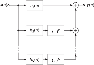
which is shown in block diagram representation in Figure 4.4. This representation shows several advantages, especially from the implementation point of view, because every subsystem can be realized by a one-dimensional impulse response. At the output of each subsystem we have to perform the ()i operation on the corresponding output signals. The discussion so far can be applied to nonlinear systems with memory, which means that besides nonlinearities linear filtering operations are also included. Further material on nonlinear audio systems can be found in [Kai87, RH96, Kli98, FUB+98].
Figure 4.4 Simulation of nonlinear systems by an N-order Volterra system model with factored kernels.
A simulation of a nonlinear system without memory, namely static nonlinear curves, can be done by a Taylor series expansion given by
4.7 
Static nonlinear curves can be applied directly to the input signal, where each input amplitude is mapped to an output amplitude according to the nonlinear function y = f[x(n)]. If one applies a squarer operation to the input signal of a given bandwidth, the output signal y(n) = x2(n) will double its bandwidth. As soon as the highest frequency after passing a nonlinear operation exceeds half the sampling frequency fs/2, aliasing will fold this frequency back to the base band. This means that for digital signals we first have to perform over-sampling of the input signal before applying any nonlinear operation to the input signal in order to avoid any aliasing distortions. This over-sampling is shown in Figure 4.5 where first up-sampling is performed and then an interpolation filter HI is used to suppress images up to the new sampling frequency Lfs. Then the nonlinear operation can be applied followed by a band-limiting filter to fs/2 and down-sampling.
Figure 4.5 Nonlinear processing by over-sampling techniques.

As can be noticed, the output spectrum only contains frequencies up to fs/2. Based on this fact the entire nonlinear processing can be performed without over-sampling and down-sampling by the system shown in Figure 4.6 [SZ99]. The input signal is split into several lowpass versions which are forwarded to an individual nonlinearity. The output signal is a weighted combination of the individual output signals after passing a nonlinearity. With this approach the problem of aliasing is avoided and an approximation to the over-sampling technique is achieved. A comparison with our previous discussion on factored Volterra kernels shows also a close connection. As a conclusion for a special static nonlinearity applied to an input signal, the input signal has to be filtered by a lowpass of cut-off frequency ![]() , otherwise aliasing distortions will occur.
, otherwise aliasing distortions will occur.
Figure 4.6 Nonlinear processing by band-limiting input range [SZ99].
