
2.6.1 Vibrato
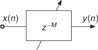
When a car is passing by, we hear a pitch deviation due to the Doppler effect [Dut91]. This effect will be explained in another chapter, but we can keep in mind that the pitch variation is due to the fact that the distance between the source and our ears is being varied. Varying the distance is, for our application, equivalent to varying the time delay. If we keep on varying periodically the time delay we will produce a periodical pitch variation. This is precisely a vibrato effect. For that purpose we need a delay line and a low-frequency oscillator to drive the delay time parameter. We should only listen to the delayed signal. Typical values of the parameters are 5 to 10 ms as the average delaytime and 5 to 14 Hz rate for the low-frequency oscillator (see Figure 2.32) [And95, Whi93]. M-file 2.8 shows the implementation for vibrato [Dis99].
M-file 2.8 (vibrato.m)
function y=vibrato(y,SAMPLERATE,Modfreq,Width)
% Author: S. Disch
ya_alt=0;
Delay=Width; % basic delay of input sample in sec
DELAY=round(Delay*SAMPLERATE); % basic delay in # samples
WIDTH=round(Width*SAMPLERATE); % modulation width in # samples
if WIDTH>DELAY
error(’delay greater than basic delay !!!’);
return;
end
MODFREQ=Modfreq/SAMPLERATE; % modulation frequency in # samples
LEN=length(x); % # of samples in WAV-file
L=2+DELAY+WIDTH*2; % length of the entire delay
Delayline=zeros(L,1); % memory allocation for delay
y=zeros(size(x)); % memory allocation for output vector
for n=1:(LEN-1)
M=MODFREQ;
MOD=sin(M*2*pi*n);
TAP=1+DELAY+WIDTH*MOD;
i=floor(TAP);
frac=TAP-i;
Delayline=[x(n);Delayline(1:L-1)];
%---Linear Interpolation-----------------------------
y(n,1)=Delayline(i+1)*frac+Delayline(i)*(1-frac);
%---Allpass Interpolation------------------------------
%y(n,1)=(Delayline(i+1)+(1-frac)*Delayline(i)-(1-frac)*ya_alt);
%ya_alt=ya(n,1);
%---Spline Interpolation-------------------------------
%y(n,1)=Delayline(i+1)*frac∧3/6
%....+Delayline(i)*((1+frac)∧3-4*frac∧3)/6
%....+Delayline(i-1)*((2-frac)∧3-4*(1-frac)∧3)/6
%....+Delayline(i-2)*(1-frac)∧3/6;
%3rd-order Spline Interpolation
end
Figure 2.32 Vibrato.
2.6.2 Flanger, Chorus, Slapback, Echo
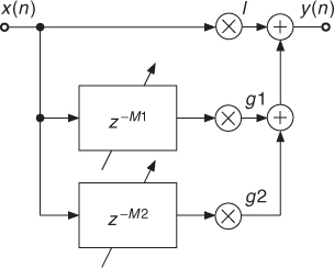
A few popular effects can be realized using the comb filter. They have special names because of the peculiar sound effects that they produce. Consider the FIR comb filter. If the delay is in the range 10 to 25 ms, we will hear a quick repetition named slapback or doubling. If the delay is greater than 50 ms we will hear an echo. If the time delay is short (less than 15 ms) and if this delay time is continuously varied with a low frequency such as 1 Hz, we will hear the flanging effect. “The flanging effect can be commonly observed outdoors, when a jet flies overhead, and the direct sound is summed in the ear of the observer with the sound reflected from the ground, resulting in the cancellation of certain frequencies and producing the comb filter effect, commonly referred to as ‘jet sound’” [Bod84]. The name “flanging” derives from alternatively braking two turntables or tape machines playing the same recording by slightly pressing a finger on their respective flange. The audio effect becomes audible by summation of the outputs of both playback devices. If several copies of the input signal are delayed in the range 10 to 25 ms with small and random variations in the delay times, we will hear the chorus effect, which is a combination of the vibrato effect with the direct signal (see Table 2.8 and Figure 2.33) [Orf96, And95, Dat97b]. The chorus effect can be interpreted as a simulation of several musicians playing the same tones, but affected by slight time and pitch variations. These effects can also be implemented as IIR comb filters. The feedback will then enhance the effect and produce repeated slapbacks or echoes.
Table 2.8 Typical delay-based effects
| Delay range (ms) | Modulation | Effect name |
| (Typ.) | (Typ.) | |
| 0 ... 20 | — | Resonator |
| 0 ... 15 | Sinusoidal | Flanging |
| 10 ... 25 | Random | Chorus |
| 25 ... 50 | — | Slapback |
| >50 | — | Echo |
Figure 2.33 Chorus.
Normalization. To avoid clipping of the output signal, it is important to compensate for the intrinsic gain of the filter structure. Whereas in practice the FIR comb filter does not amplify the signal by more than 6 dB, the IIR comb filter can yield a very large amplification when |g| comes close to 1. The L2 and L∞ norms are given by
2.67 ![]()
The normalization coefficient c = 1/L∞, when applied, ensures that no overload will occur with, for example, periodical input signals. c = 1/L2 ensures that the loudness will remain approximatively constant for broadband signals.
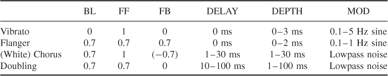
A standard effect structure was proposed by Dattorro [Dat97b] and is shown in Figure 2.34. It is based on the allpass filter modification towards a general allpass comb, where the fixed delay line is replaced by a variable-length delay line. Dattorro [Dat97b] proposed keeping the feedback tap of the delay line fixed, that means the input signal to the delay line xh(n) is delayed by a fixed integer delay K and with this xh(n − K) is weighted and fed back. The delay K is the center tab delay of the variable-length delay line for the feed forward path. The control signal MOD(n) for changing the length of the delay line can either be a sinusoid or lowpass noise. Typical settings of the parameters are given in Table 2.9.
Figure 2.34 Standard effects with variable-length delay line.
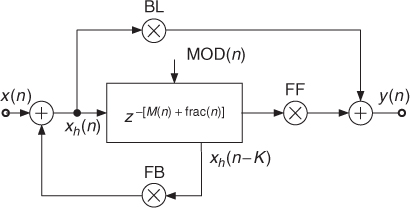
Table 2.9 Industry standard audio effects. [Dis99]
2.6.3 Multiband Effects
New interesting sounds can be achieved after splitting the signal into several frequency bands, for example, lowpass, bandpass and highpass signals, as shown in Figure 2.35.
Figure 2.35 Multiband effects.

Variable-length delays are applied to these signals with individual parameter settings and the output signals are weighted and summed to the broadband signal [FC98, Dis99]. Efficient frequency-splitting schemes are available from loudspeaker crossover designs and can be applied for this purpose directly. One of these techniques uses complementary filtering [Fli94, Orf96], which consists of lowpass filtering and subtracting the lowpass signal from the broadband signal to derive the highpass signal, as shown in Figure 2.36. The lowpass signal is then further processed by a following stage of the same complementary technique to deliver the bandpass and lowpass signals.
Figure 2.36 Filter bank for multiband effects.

2.6.4 Natural Sounding Comb Filter
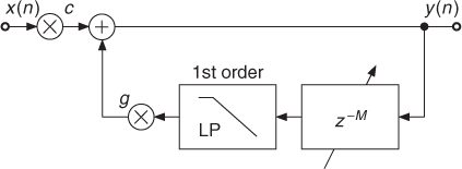
We have made the comparison between acoustical cylinders and IIR comb filters. This comparison might seem inappropriate because the comb filters sound metallic. They tend to amplify greatly the high-frequency components and they appear to resonate much too long compared to the acoustical cylinder. To find an explanation, let us consider the boundaries of the cylinder. They reflect the acoustic waves with an amplitude that decreases with frequency. If the comb filter should sound like an acoustical cylinder, then it should also have a frequency-dependent feedback coefficient g(f). This frequency dependence can be realized by using a first-order lowpass filter in the feedback loop (see Figure 2.37) [Moo85].
Figure 2.37 Lowpass IIR comb filter.
These filters sound more natural than the plain IIR comb filters. They find application in room simulators. Further refinements such as fractional delays and compensation of the frequency-dependent group delay within the lowpass filter make them suitable for the imitation of acoustical resonators. They have been used, for example, to impose a definite pitch onto broadband signals such as sea waves or to detune fixed-pitched instruments such as a Celtic harp [m-Ris92]. M-file 2.9 shows the implementation for a sample-by-sample based lowpass IIR comb filter.
M-file 2.9 (lpiircomb.m)
% Authors: P.Dutilleux, U. Zölzer
x=zeros(100,1);x(1)=1; % unit impulse signal of length 100
g=0.5;
b_0=0.5;
b_1=0.5;
a_1=0.7;
xhold=0;yhold=0;
Delayline=zeros(10,1); % memory allocation for length 10
for n=1:length(x);
yh(n)=b_0*Delayline(10)+b_1*xhold-a_1*yhold;
% 1st-order difference equation
yhold=yh(n);
xhhold=Delayline(10);
y(n)=x(n)+g*yh(n);
Delayline=[y(n);Delayline(1:10-1)];
end;