7.3 Phase Vocoder Implementations
This section describes several phase vocoder implementations for digital audio effects. A useful representation is the time-frequency plane where one displays the values of the magnitude |X(n, k)| and phase ![]() of the
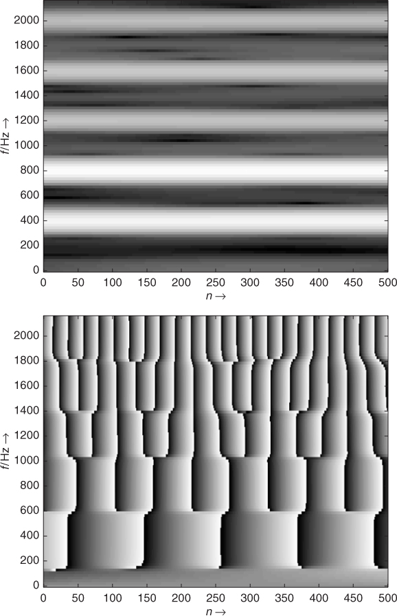
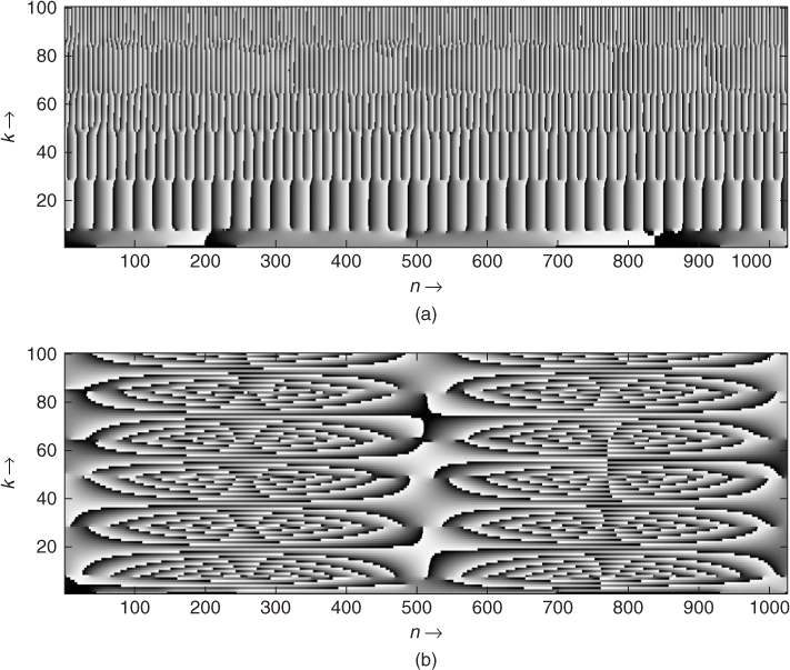
of the ![]() signal. If the sliding Fourier transform is used as an analysis scheme, this graphical representation is the combination of the spectrogram, which displays the magnitude values of this representation, and the phasogram, which displays the phase. However, phasograms are harder to read when the hop size is not small. Figure 7.6 shows a spectrogram and a phasogram which correspond to the discrete-time and discrete-frequency plane achieved by a filter bank (see Figure 7.4) or a block-by-block FFT analysis (see Figure 7.5) described in the previous section. In the horizontal direction a line represents the output magnitude |X(n, k)| and the phase
signal. If the sliding Fourier transform is used as an analysis scheme, this graphical representation is the combination of the spectrogram, which displays the magnitude values of this representation, and the phasogram, which displays the phase. However, phasograms are harder to read when the hop size is not small. Figure 7.6 shows a spectrogram and a phasogram which correspond to the discrete-time and discrete-frequency plane achieved by a filter bank (see Figure 7.4) or a block-by-block FFT analysis (see Figure 7.5) described in the previous section. In the horizontal direction a line represents the output magnitude |X(n, k)| and the phase ![]() of the kth analysis bandpass filter over the time index n. In the vertical direction a line represents the magnitude |X(n, k)| and phase
of the kth analysis bandpass filter over the time index n. In the vertical direction a line represents the magnitude |X(n, k)| and phase ![]() for a fixed time index n, which corresponds to a short-time spectrum over frequency bin k at the center of the analysis window located at time index n. The spectrogram in Figure 7.6 with frequency range up to 2 kHz shows five horizontal rays over the time axis, indicating the magnitude of the harmonics of the analyzed sound segment. The phasogram shows the corresponding phases for all five horizontal rays
for a fixed time index n, which corresponds to a short-time spectrum over frequency bin k at the center of the analysis window located at time index n. The spectrogram in Figure 7.6 with frequency range up to 2 kHz shows five horizontal rays over the time axis, indicating the magnitude of the harmonics of the analyzed sound segment. The phasogram shows the corresponding phases for all five horizontal rays ![]() , which rotate according to the frequencies of the five harmonics. With a hop size of one we get a visible tree structure. For a larger hop size we get a sampled version, where the tree structure usually disappears.
, which rotate according to the frequencies of the five harmonics. With a hop size of one we get a visible tree structure. For a larger hop size we get a sampled version, where the tree structure usually disappears.
Figure 7.6 Magnitude |X(n, k)| (upper plot) and phase ![]() (lower plot) display of a sliding Fourier transform with a hop size Ra = 1 or a filter-bank analysis approach. For the upper display the grey value (black = 0 and white = maximum amplitude) represents the magnitude range. In the lower display the phase values are in the range
(lower plot) display of a sliding Fourier transform with a hop size Ra = 1 or a filter-bank analysis approach. For the upper display the grey value (black = 0 and white = maximum amplitude) represents the magnitude range. In the lower display the phase values are in the range ![]() .
.
The analysis and synthesis part can come from the filter bank summation model (see basics), in which case the resynthesis part consists in summing sinusoids, whose amplitudes and frequencies are coming from a parallel bank of filters. The analysis part can also come from a sliding FFT algorithm, in which case it is possible to perform the resynthesis with either a summation of sinusoids or an IFFT approach.
7.3.1 Filter Bank Approach
From a musician's point of view the idea behind this technique is to represent a sound signal as a sum of sinusoids. Each of these sinusoids is modulated in amplitude and frequency. They represent filtered versions of the original signal. The manipulation of the amplitudes and frequencies of these individual signals will produce a digital effect, including time stretching or pitch shifting.
One can use a filter bank, as shown in Figure 7.7, to split the audio signal into several filtered versions. The sum of these filtered versions reproduces the original signal. For a perfect reconstruction the sum of the filter frequency responses should be unity. In order to produce a digital audio effect, one needs to alter the intermediate signals that are analytical signals consisting of real and imaginary parts (double lines in Figure 7.7). The implementation of each filter can be performed by a heterodyne filter, as shown in Figure 7.8.
Figure 7.7 Filter-bank implementation.
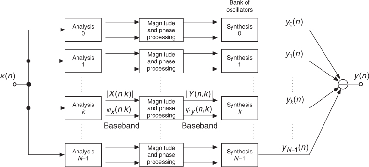
Figure 7.8 Heterodyne-filter implementation.

The implementation of a stage of a heterodyne filter consists of a complex-valued oscillator with a fixed frequency ωk, a multiplier and an FIR filter. The multiplication shifts the spectrum of the sound, and the FIR filter limits the width of the frequency-shifted spectrum. This heterodyne filtering can be used to obtain intermediate analytic signals, which can be put in the form
7.24 ![]()
7.25 ![]()
7.26 ![]()
7.27 ![]()
The difference from classical bandpass filtering is that here the output signal is located in the baseband. This representation leads to a slowly varying phase φ(n, k) and the derivation of the phase is a measure of the frequency deviation from the center frequency ωk. A sinusoid x(n) = cos[ωkn + φ0] with frequency ωk can be written as ![]() , where
, where ![]() . The derivation of
. The derivation of ![]() gives the frequency
gives the frequency ![]() . The derivation of the phase
. The derivation of the phase ![]() at the output of a bandpass filter is termed the instantaneous frequency given by
at the output of a bandpass filter is termed the instantaneous frequency given by
7.28 ![]()
7.29 ![]()
7.30 ![]()
7.31 ![]()
7.32 ![]()
The instantaneous frequency can be described in a musical way as the frequency of the filter output signal in the filter-bank approach. The phase of the baseband output signal is φ(n, k) and the phase of the bandpass output signal is ![]() (see Figure 7.8). As soon as we have the instantaneous frequencies, we can build an oscillator bank and eventually change the amplitudes and frequencies of this bank to build a digital audio effect. The recalculation of the phase from a modified instantaneous frequency is done by computing the phase according to
(see Figure 7.8). As soon as we have the instantaneous frequencies, we can build an oscillator bank and eventually change the amplitudes and frequencies of this bank to build a digital audio effect. The recalculation of the phase from a modified instantaneous frequency is done by computing the phase according to
7.33 ![]()
The result of the magnitude and phase processing can be written as ![]() , which is then used as the magnitude and phase for the complex-valued oscillator running with frequency ωk. The output signal is then given by
, which is then used as the magnitude and phase for the complex-valued oscillator running with frequency ωk. The output signal is then given by
7.34 ![]()
7.35 ![]()
The resynthesis of the output signal can then be performed by summing all the individual back-shifted signals (oscillator bank) according to
7.36 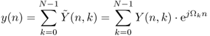
where (7.37) was already introduced by (7.18). The modification of the phases and frequencies for time stretching and pitch shifting needs further explanation and will be treated in a following subsection.
The following M-file 7.1 shows a filter-bank implementation with heterodyne filters, as shown in Figure 7.8 (see also Figure 7.4).
M-file 7.1 (VX_het_nothing.m)
% VX_het_nothing.m [DAFXbook, 2nd ed., chapter 7]
clear; clf
%===== This program (i) implements a heterodyne filter bank,
%===== then (ii) filters a sound through the filter bank
%===== and (iii) reconstructs a sound
%----- user data -----
fig_plot = 0; % use any value except 0 or [] to plot figures
s_win = 256; % window size
n_channel = 128; % nb of channels
s_block = 1024; % computation block size (must be a multiple of s_win)
[DAFx_in, FS] = wavread(‘la.wav’);
%----- initialize windows, arrays, etc -----
window = hanning(s_win, ‘periodic’);
s_buffer = length(DAFx_in);
DAFx_in = [DAFx_in; zeros(s_block,1)]/ max(abs(DAFx_in)); % 0-pad & normalize
DAFx_out = zeros(length(DAFx_in),1);
X = zeros(s_block, n_channel);
z = zeros(s_win-1, n_channel);
%----- initialize the heterodyn filters -----
t = (0:s_block-1)';
het = zeros(s_block,n_channel);
for k=1:n_channel
wk = 2*pi*i*(k/s_win);
het(:,k) = exp(wk*(t+s_win/2));
het2(:,k) = exp(-wk*t);
end
%----- displays the phase of the filter -----
if(fig_plot)
colormap(gray); imagesc(angle(het)'), colorbar;
axis(‘xy’); xlabel(‘n ightarrow’); ylabel(‘k ightarrow’);
title(‘Heterodyn filter bank: initial phi(n,k)’); pause;
end
tic
%UUUUUUUUUUUUUUUUUUUUUUUUUUUUUUUUUUUUUUU
pin = 0;
pend = length(DAFx_in) - s_block;
while pin<pend
grain = DAFx_in(pin+1:pin+s_block);
%===========================================
%----- filtering through the filter bank -----
for k=1:n_channel
[X(:,k), z(:,k)] = filter(window, 1, grain.*het(:,k), z(:,k));
end
X_tilde = X.*het2;
%----- drawing -----
if(fig_plot)
imagesc(angle(X_tilde')); axis(‘xy’); colorbar;
xlabel(‘n ightarrow’); ylabel(‘k ightarrow’);
txt = sprintf(‘Heterodyn filter bank: \phi(n,k),t=%6.3f s’,(pin+1)/FS);
title(txt); drawnow;
end
%----- sound reconstruction -----
res = real(sum(X_tilde,2));
%===========================================
DAFx_out(pin+1:pin+s_block) = res;
pin = pin + s_block;
end
%UUUUUUUUUUUUUUUUUUUUUUUUUUUUUUUUUUUUUUU
toc
%----- listening and saving the output -----
DAFx_out = DAFx_out(n_channel+1:n_channel+s_buffer) / max(abs(DAFx_out));
soundsc(DAFx_out, FS);
wavwrite(DAFx_out, FS, ‘la_het_nothing.wav’);
M-file 7.2 demonstrates the second-filter bank implementation with complex-valued bandpass filters, as shown in Figure 7.4.
M-file 7.2 (VX_filter_nothing.m)
% VX_filter_nothing.m [DAFXbook, 2nd ed., chapter 7]
clear; clf
%===== This program (i) performs a complex-valued filter bank
%===== then (ii) filters a sound through the filter bank
%===== and (iii) reconstructs a sound
%----- user data -----
fig_plot = 0; % use any value except 0 or [] to plot figures
s_win = 256; % window size
nChannel = 128; % nb of channels
n1 = 1024; % block size for calculation
[DAFx_in,FS] = wavread(‘la.wav’);
%----- initialize windows, arrays, etc -----
window = hanning(s_win, ‘periodic’);
L = length(DAFx_in);
DAFx_in = [DAFx_in; zeros(n1,1)] / max(abs(DAFx_in)); % 0-pad & normalize
DAFx_out = zeros(length(DAFx_in),1);
X_tilde = zeros(n1,nChannel);
z = zeros(s_win-1,nChannel);
%----- initialize the complex-valued filter bank -----
t = (-s_win/2:s_win/2-1)';
filt = zeros(s_win, nChannel);
for k=1:nChannel
wk = 2*pi*i*(k/s_win);
filt(:,k) = window.*exp(wk*t);
end
if(fig_plot), colormap(gray); end
tic
%UUUUUUUUUUUUUUUUUUUUUUUUUUUUUUUUUUUUUUU
pin = 0;
pend = length(DAFx_in) - n1;
while pin<pend
grain = DAFx_in(pin+1:pin+n1);
%===========================================
%----- filtering -----
for k=1:nChannel
[X_tilde(:,k),z(:,k)] = filter(filt(:,k),1,grain,z(:,k));
end
if(fig_plot)
imagesc(angle(X_tilde')); axis(‘xy’); colorbar;
xlabel(‘n ightarrow’); ylabel(‘k ightarrow’);
txt = sprintf(‘Complex-valued fil. bank: \phi(n,k), t=%6.3f s’, (pin+1)/FS);
title(txt); drawnow;
end
%----- sound reconstruction -----
res = real(sum(X_tilde,2));
%===========================================
DAFx_out(pin+1:pin+n1) = res;
pin = pin + n1;
end
%UUUUUUUUUUUUUUUUUUUUUUUUUUUUUUUUUUUUUUU
toc
%----- listening and saving the output -----
DAFx_out = DAFx_out(nChannel+1:nChannel+L) / max(abs(DAFx_out));
soundsc(DAFx_out, FS);
wavwrite(DAFx_out, FS, ‘la_filter_nothing.wav’);
7.3.2 Direct FFT/IFFT Approach
The FFT algorithm also calculates the values of the magnitudes and phases within a time frame, allowing a shorter calculation time. So many analysis-synthesis algorithms use this transform. There are different ways to interpret a sliding Fourier transform, and consequently to invent a method of resynthesis starting from this time-frequency representation. The first one is to apply the inverse FFT on each short-time spectrum and use the overlap-add method to reconstruct the signal. The second one is to consider a horizontal line of the time-frequency representation (constant frequency versus time) and to reconstruct a filtered version for each line. The third one is to consider each point of the time-frequency representation and to make a sum of small grains called gaborets. In each interpretation one must test the ability of obtaining a perfect reconstruction if one does not modify the representation. Another important fact is the ability to provide effect implementations that do not have too many artifacts when one modifies on purpose the values of the sliding FFT, especially in operations such as time stretching or filtering.
We now describe the direct FFT/IFFT approach. A time-frequency representation can be seen as a series of overlapping FFTs with or without windowing. As the FFT is invertible, one can reconstruct a sound by adding the inverse FFT of a vertical line (constant time versus frequency), as shown in Figure 7.9.
Figure 7.9 FFT and IFFT: vertical line interpretation. At two time instances two spectra are used to compute two time segments.
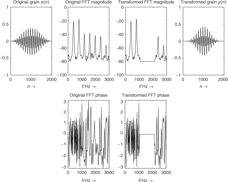
A perfect reconstruction can be achieved, if the sum of the overlapping windows is unity (see Figure 7.10). A modification of the FFT values can produce time aliasing, which can be avoided by either zero-padded windows or using windowing after the inverse FFT. In this case the product of the two windows has to be unity. An example is shown in Figure 7.11. This implementation will be used most frequently in this chapter.
Figure 7.10 Sum of small windows.
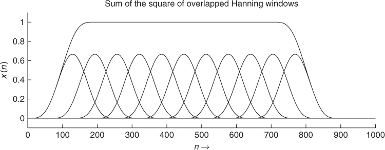
Figure 7.11 Sound windowing, FFT modification and IFFT.
The following M-file 7.3 shows a phase vocoder implementation based on the direct FFT/IFFT approach, where the routine itself is given two vectors for the sound, a window and a hop size.
M-file 7.3 (VX_pv_nothing.m)
% VX_pv_nothing.m [DAFXbook, 2nd ed., chapter 7]
%===== this program implements a simple phase vocoder
clear; clf
%----- user data -----
fig_plot = 0; % use any value except 0 or [] to plot figures
n1 = 512; % analysis step [samples]
n2 = n1; % synthesis step [samples]
s_win = 2048; % window size [samples]
[DAFx_in, FS] = wavread(‘la.wav’);
%----- initialize windows, arrays, etc -----
w1 = hanning(s_win, ‘periodic’); % input window
w2 = w1; % output window
L = length(DAFx_in);
DAFx_in = [zeros(s_win, 1); DAFx_in; ...
zeros(s_win-mod(L,n1),1)] / max(abs(DAFx_in)); % 0-pad & normalize
DAFx_out = zeros(length(DAFx_in),1);
tic
%UUUUUUUUUUUUUUUUUUUUUUUUUUUUUUUUUUUUUUU
pin = 0;
pout = 0;
pend = length(DAFx_in) - s_win;
while pin<pend
grain = DAFx_in(pin+1:pin+s_win).* w1;
%===========================================
f = fft(fftshift(grain)); % FFT
r = abs(f); % magnitude
phi = angle(f); % phase
ft = (r.* exp(i*phi)); % reconstructed FFT
grain = fftshift(real(ifft(ft))).*w2;
% ===========================================
DAFx_out(pout+1:pout+s_win) = ...
DAFx_out(pout+1:pout+s_win) + grain;
pin = pin + n1;
pout = pout + n2;
end
%UUUUUUUUUUUUUUUUUUUUUUUUUUUUUUUUUUUUUUU
toc
%----- listening and saving the output -----
% DAFx_in = DAFx_in(s_win+1:s_win+L);
DAFx_out = DAFx_out(s_win+1:s_win+L) / max(abs(DAFx_out));
soundsc(DAFx_out, FS);
wavwrite(DAFx_out, FS, ‘la_pv_nothing.wav’);
The kernel algorithm performs successive FFTs, inverse FFTs and overlap-add of successive grains. The key point of the implementations is how to go from the FFT representation, where the time origin is at the beginning of the window, to the phase vocoder representation used in Section 7.2, either in its filter-bank description or its block-by-block approach.
The first problem we have to solve is the fact that the time origin for an FFT is on the left of the window. We would like to have it centered, so that, for example, the FFT of a centered impulse would be zero phase. This is done by a circular shift of the signal, which is a commutation of the first and second part of the buffer. The discrete-time Fourier transform of ![]() is
is ![]() . With
. With ![]() the discrete Fourier transform gives
the discrete Fourier transform gives ![]() , which is equivalent to
, which is equivalent to ![]() . The circular shift in time domain can be achieved by multiplying the result of the FFT by (−1)k. With this circular shift, the output of the FFT is equivalent to a filter bank, with zero phase filters. When analyzing a sine wave, the display of the values of the phase
. The circular shift in time domain can be achieved by multiplying the result of the FFT by (−1)k. With this circular shift, the output of the FFT is equivalent to a filter bank, with zero phase filters. When analyzing a sine wave, the display of the values of the phase ![]() of the time-frequency representation will follow the phase of the sinusoid. When analyzing a harmonic sound, one obtains a tree with successive branches corresponding to every harmonic (top of Figure 7.12).
of the time-frequency representation will follow the phase of the sinusoid. When analyzing a harmonic sound, one obtains a tree with successive branches corresponding to every harmonic (top of Figure 7.12).
Figure 7.12 Different phase representations: (a) ![]() and (b)
and (b) ![]() .
.
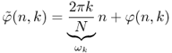
If we want to take an absolute value as the origin of time, we have to switch to the notation used in Section 7.2. We have to multiply the result of the FFT by ![]() , where m is the time sample in the middle of the FFT and k is the number of the bin of the FFT. In this way the display of the phase φ(n, k) (bottom of Figure 7.12) corresponds to a frequency which is the difference between the frequency of the analyzed signal (here a sine wave) delivered by the FFT and the analyzing frequency (the center of the bin). The phase φ(n, k) is calculated as
, where m is the time sample in the middle of the FFT and k is the number of the bin of the FFT. In this way the display of the phase φ(n, k) (bottom of Figure 7.12) corresponds to a frequency which is the difference between the frequency of the analyzed signal (here a sine wave) delivered by the FFT and the analyzing frequency (the center of the bin). The phase φ(n, k) is calculated as ![]() (N length of FFT, k number of the bin, m time index).
(N length of FFT, k number of the bin, m time index).
7.3.3 FFT Analysis/sum of Sinusoids Approach
Conversely, one can read a time-frequency representation with horizontal lines, as shown in Figure 7.13. Each point on a horizontal line can be seen as the convolution of the original signal with an FIR filter, whose filter coefficients have been given by (7.4). The filter-bank approach is very close to the heterodyne-filter implementation. The difference comes from the fact that for heterodyne filtering the complex exponential is running with time and the sliding FFT is considering for each point the same phase initiation of the complex exponential. It means that the heterodyne filter measures the phase deviation between a cosine and the filtered signal, and the sliding FFT measures the phase with a time origin at zero.
Figure 7.13 Filter-bank approach: horizontal line interpretation.
The reconstruction of a sliding FFT on a horizontal line with a hop size of one is performed by filtering of this line with the filter corresponding to the frequency bin (see Figure 7.13). However, if the analysis hop size is greater than one, we need to interpolate the magnitude values |X(n, k)| and phase values ![]() . Phase interpolation is based on phase unwrapping, which will be explained in Section 7.3.5. Combining phase interpolation with linear interpolation of the magnitudes |X(n, k)| allows the reconstruction of the sound by the addition of a bank of oscillators, as given in (7.37).
. Phase interpolation is based on phase unwrapping, which will be explained in Section 7.3.5. Combining phase interpolation with linear interpolation of the magnitudes |X(n, k)| allows the reconstruction of the sound by the addition of a bank of oscillators, as given in (7.37).
M-file 7.4 illustrates the interpolation and the sum of sinusoids. Starting from the magnitudes and phases taken from a sliding FFT the synthesis implementation is performed by a bank of oscillators. It uses linear interpolation of the magnitudes and phases.
M-file 7.4 (VX_bank_nothing.m)
% VX_bank_nothing.m [DAFXbook, 2nd ed., chapter 7]
%===== This program performs an FFT analysis and oscillator bank synthesis
clear; clf
%----- user data -----
n1 = 200; % analysis step [samples]
n2 = n1; % synthesis step [samples]
s_win = 2048; % window size [samples]
[DAFx_in, FS] = wavread(‘la.wav’);
%----- initialize windows, arrays, etc -----
w1 = hanning(s_win, ‘periodic’); % input window
w2 = w1; % output window
L = length(DAFx_in);
DAFx_in = [zeros(s_win, 1); DAFx_in; ...
zeros(s_win-mod(L,n1),1)] / max(abs(DAFx_in)); % 0-pad & normalize
DAFx_out = zeros(length(DAFx_in),1);
ll = s_win/2;
omega = 2*pi*n1*[0:ll-1]'/s_win;
phi0 = zeros(ll,1);
r0 = zeros(ll,1);
psi = zeros(ll,1);
grain = zeros(s_win,1);
res = zeros(n2,1);
tic
%UUUUUUUUUUUUUUUUUUUUUUUUUUUUUUUUUUUUUUU
pin = 0;
pout = 0;
pend = length(DAFx_in) - s_win;
while pin<pend
grain = DAFx_in(pin+1:pin+s_win).* w1;
%===========================================
fc = fft(fftshift(grain)); % FFT
f = fc(1:ll); % positive frequency spectrum
r = abs(f); % magnitudes
phi = angle(f); % phases
%----- unwrapped phase difference on each bin for a n2 step
delta_phi = omega + princarg(phi-phi0-omega);
%----- phase and magnitude increment, for linear
% interpolation and reconstruction -----
delta_r = (r-r0)/n1; % magnitude increment
delta_psi = delta_phi/n1; % phase increment
for k=1:n2 % compute the sum of weighted cosine
r0 = r0 + delta_r;
psi = psi + delta_psi;
res(k) = r0'*cos(psi);
end
%----- for next time -----
phi0 = phi;
r0 = r;
psi = princarg(psi);
% ===========================================
DAFx_out(pout+1:pout+n2) = DAFx_out(pout+1:pout+n2) + res;
pin = pin + n1;
pout = pout + n2;
end
%UUUUUUUUUUUUUUUUUUUUUUUUUUUUUUUUUUUUUUU
toc
%----- listening and saving the output -----
% DAFx_in = DAFx_in(s_win+1:s_win+L);
DAFx_out = DAFx_out(s_win/2+n1+1:s_win/2+n1+L) / max(abs(DAFx_out));
soundsc(DAFx_out,FS);
wavwrite(DAFx_out, FS, ‘la_bank_nothing.wav’);
7.3.4 Gaboret Approach
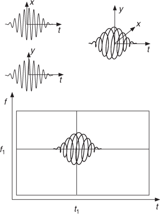
The idea of the “gaboret approach” is the reconstruction of a signal from a time-frequency representation with the sum of “gaborets” weighted by the values of the time-frequency representation [AD93]. The shape of a gaboret is a windowed exponential (see Figure 7.14), which can be given by ![]() . The approach is based on the Gabor transform, which is a short-time Fourier transform with the smallest time-frequency window, namely a Gaussian function
. The approach is based on the Gabor transform, which is a short-time Fourier transform with the smallest time-frequency window, namely a Gaussian function ![]() with α > 0. The discrete-time Fourier transform of gα(n) is again a Gaussian function in the Fourier domain. The gaboret approach is very similar to the wavelet transform [CGT89, Chu92]: one does not consider time or frequency as a privileged axis and one point of the time-frequency plane is the scalar product of the signal with a small gaboret. Further details can be found in [QC93, WR90]. The reconstruction from a time-frequency representation is the sum of gaborets weighted by the values of this time-frequency plane according to
with α > 0. The discrete-time Fourier transform of gα(n) is again a Gaussian function in the Fourier domain. The gaboret approach is very similar to the wavelet transform [CGT89, Chu92]: one does not consider time or frequency as a privileged axis and one point of the time-frequency plane is the scalar product of the signal with a small gaboret. Further details can be found in [QC93, WR90]. The reconstruction from a time-frequency representation is the sum of gaborets weighted by the values of this time-frequency plane according to
7.38 
Although this point of view is totally equivalent to windowing plus FFT/IFFT plus windowing, it allows a good comprehension of what happens in case of modification of a point in the plane.
Figure 7.14 Gaboret approach: the upper left part shows real and imaginary values of a gaboret and the upper right part shows a possible 3D repesentation with axes t, x and y. The lower part shows a gaboret associated to a specific point of a time-frequency representation (for every point we can generate a gaboret in the time domain and then make the sum of all gaborets).
The reconstruction of one single point of a time-frequency representation yields a gaboret in the time domain, as shown in Figure 7.15. Then a new time-frequency representation of this gaboret is computed. We get a new image, which is the called the reproducing kernel associated with the transform. This new time-frequency representation is different from the single point of the original time-frequency representation.
Figure 7.15 Reproducing kernel: the lower three plots represent the forced gaboret and the reproducing kernel consisting of spectrogram and phasogram. (Note: phase values only make sense when the magnitude is not too small.)
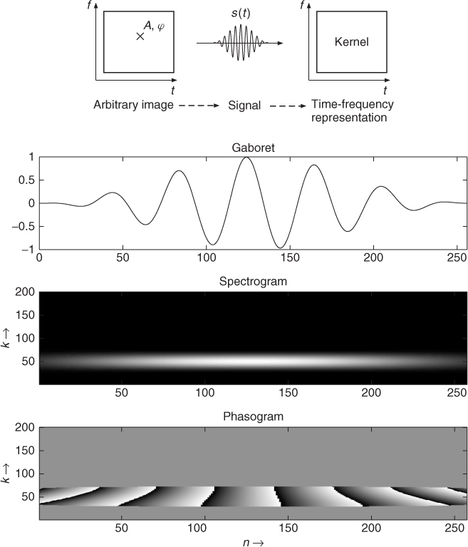
So a time-frequency representation of a real signal has some constraints: each value of the time-frequency plane must be the convolution of the neighborhood by the reproducing kernel associated with the transformation. This means that if an image (time-frequency representation) is not valid and if we force the reconstruction of a sound by the weighted summation of gaborets, the time-frequency representation of this transformed sound will be in a different form than the initial time-frequency representation. There is no way to avoid this and the beautiful art of making good transforms often relies on the ability to provide “quasi-valid” representations [AD93].
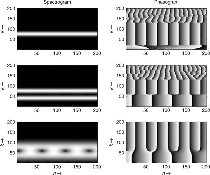
This reproducing kernel is only a 2 D extension of the well-known problem of windowing: we find the shape of the FFT of the window around one horizontal ray. But it brings new aspects. When we have two spectral lines, their time-frequency representations are blurred and, when summed, appear as beats. Illustrative examples are shown in Figure 7.16. The shape of the reproducing kernel depends on the shape of the window and is the key point for differences in representations between different windows. The matter of finding spectral lines starting from time-frequency representations is the subject of Chapter 10. Here we only consider the fact that any signal can be generated as the sum of small gaborets. Frequency estimations in bins are obviously biased by the interaction between rays and additional noise.
Figure 7.16 Spectrogram and phasogram examples: (a) upper part: the effect of the reproducing kernel is to thicken the line and giving a rotating phase at the frequency of the sinusoid; (b) middle part: for two sinusoids we have two lines with two rotations, if the window is large; (c) lower part: for two sinusoids with a shorter window the two lines mix and we can see beating.
The following M-file 7.5 demonstrates the gaboret analysis and synthesis approach.
M-file 7.5 (VX_gab_nothing.m)
% VX_gab_nothing.m [DAFXbook, 2nd ed., chapter 7]
%==== This program performs signal convolution with gaborets
clear; clf
%----- user data -----
n1 = 128; % analysis step [samples]
n2 = n1; % synthesis step [samples]
s_win = 512; % window size [samples]
[DAFx_in, FS] = wavread(‘la.wav’);
%----- initialize windows, arrays, etc -----
window = hanning(s_win, ‘periodic’); % input window
nChannel = s_win/2;
L = length(DAFx_in);
DAFx_in = [zeros(s_win, 1); DAFx_in; ...
zeros(s_win-mod(L,n1),1)] / max(abs(DAFx_in));
DAFx_out = zeros(length(DAFx_in),1); % 0-pad & normalize
%----- initialize calculation of gaborets -----
t = (-s_win/2:s_win/2-1);
gab = zeros(nChannel,s_win);
for k=1:nChannel
wk = 2*pi*i*(k/s_win);
gab(k,:) = window'.*exp(wk*t);
end
tic
%UUUUUUUUUUUUUUUUUUUUUUUUUUUUUUUUUUUUUUU
pin = 0;
pout = 0;
pend = length(DAFx_in) - s_win;
while pin<pend
grain = DAFx_in(pin+1:pin+s_win);
%===========================================
%----- complex vector corresponding to a vertical line
vec = gab*grain;
%----- reconstruction from the vector to a grain
res = real(gab'*vec);
% ===========================================
DAFx_out(pout+1:pout+s_win) = DAFx_out(pout+1:pout+s_win) + res;
pin = pin + n1;
pout = pout + n2;
end
%UUUUUUUUUUUUUUUUUUUUUUUUUUUUUUUUUUUUUUU
toc
%----- listening and saving the output -----
% DAFx_in = DAFx_in(s_win+1:s_win+L);
DAFx_out = DAFx_out(s_win+1:s_win+L) / max(abs(DAFx_out));
soundsc(DAFx_out, FS);
wavwrite(DAFx_out, FS, ‘la_gab_nothing.wav’);
7.3.5 Phase Unwrapping and Instantaneous Frequency
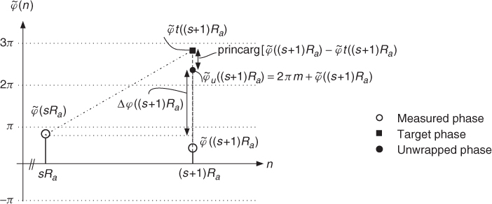
For the tasks of phase interpolation and instantaneous frequency calculation, for every frequency bin k we need a phase unwrapping algorithm. Starting from Figure 7.4 we perform unwrapping of
by unwrapping φ(n, k) and adding the phase variation given by ωkn for all k, as already shown by (7.10). We also need a special function which puts an arbitrary radian phase value into the range [−π, π]. We will call this function principle argument [GBA00], which is defined by the expression ![]() , where −π < φx ≤ π and m is an integer number. The corresponding MATLAB® function is shown in Figure 7.17.
, where −π < φx ≤ π and m is an integer number. The corresponding MATLAB® function is shown in Figure 7.17.
Figure 7.17 Principle argument function (MATLAB code and illustrative plot).
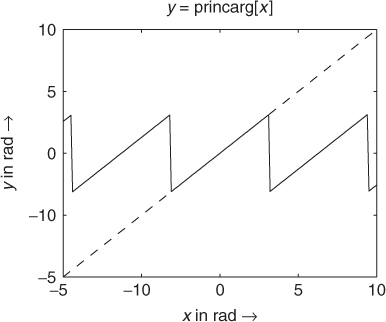
M-file 7.6 (princarg.m)
function phase = princarg(phase_in)
% This function puts an arbitrary phase value into ]-pi,pi] [rad]
phase = mod(phase_in + pi,−2*pi) + pi;
The phase computations are based on the phase values ![]() and
and ![]() , which are the results of the FFTs of two consecutive frames. These phase values are shown in Figure 7.18. We now consider the phase values regardless of the frequency bin k. If a stable sinusoid with frequency ωk exists, we can compute a target phase
, which are the results of the FFTs of two consecutive frames. These phase values are shown in Figure 7.18. We now consider the phase values regardless of the frequency bin k. If a stable sinusoid with frequency ωk exists, we can compute a target phase ![]() from the previous phase value
from the previous phase value ![]() according to
according to
7.39 ![]()
The unwrapped phase
is computed by the target phase ![]() plus a deviation phase
plus a deviation phase ![]() . This deviation phase can be computed by the measured phase
. This deviation phase can be computed by the measured phase ![]() and the target phase
and the target phase ![]() according to
according to
Now we formulate the unwrapped phase (7.40) with the deviation phase (7.41), which leads to the expression
![]()
From the previous equation we can derive the unwrapped phase difference
7.42 ![]()
between two consecutive frames. From this unwrapped phase difference we can calculate the instantaneous frequency for frequency bin k at time instant (s + 1)Ra by
7.43 ![]()
The MATLAB instructions for the computation of the unwrapped phase difference given by (7.41) for every frequency bin k are given here:
omega = 2*pi*n1*[0:ll-1]’ / s_win;
% ll = N/2 % with N length of the FFT
% n1 = R_a
delta_phi = omega + princarg(phi - phi0 - omega);
The term phi represents ![]() and phi0 the previous phase value
and phi0 the previous phase value ![]() . In this manner delta_phi represents the unwrapped phase variation Δφ((s + 1)Ra) between two successive frames for every frequency bin k.
. In this manner delta_phi represents the unwrapped phase variation Δφ((s + 1)Ra) between two successive frames for every frequency bin k.
Figure 7.18 Basics of phase computations for frequency bin k.