
9.2.1 General Comments
Sound features are parameters that describe the sound. They are used in a wide variety of applications such as coding, automatic transcription, automatic score following, and analysis-synthesis. As an example, the research field of music information retrieval has been rapidly and increasingly developing during the last ten years, offering various analysis systems and many sound features. A musical sound has some perceptive features that can be extracted from a time-frequency representation. As an example, pitch is a function of time that is very important for musicians, but richness of timbre, inharmonicity, balance between odd and even harmonics, and noise level are other examples of such time-varying parameters. These parameters are global in the sense that they are observations of the sound without any analytical separation of these components, which will be discussed in Chapter 10. They are related to perceptive cues and are based on hearing and psychoacoustics. These global parameters can be extracted from time-frequency or source-filter representations using classical tools of signal processing, where psychoacoustic fundamentals also have to be taken into account. The use of these parameters for digital audio effects is twofold: one can use them inside the effect algorithm itself, or one can use these features as control variables for other effects, which is the purpose of this chapter. Pitch tracking as a source of control is a well-known application. Examples of audio effects using feature extraction inside the algorithm are the correction of tuning, which uses pitch extraction (auto-tune), or even the compression of a sound, which uses amplitude extraction.
Their computation is based on a representation of the sound (for instance a source-filter, a time-frequency or a spectral model), but not necessarily the same as the one used to apply the adaptive effect. This means that the two signal-processing blocks of sound-feature extraction and audio effect may be decorrelated, and the implementation of one may not rely on the implementation of the other, resulting in an increase in CPU use. For this reason, we will present the computation of various sound features, each with various implementations, depending on the model domain. Depending on the application, sound features may require more- or less-accurate computation. For instance, an automatic score-following system must have accurate pitch and rhythm detection. Another example is the evaluation of brightness, acoustical correlate of which is the spectral centroid. Therefore, brightness can either be computed from a psychoacoustic model of brightness [vA85, ZF99], or approximated by the spectral centroid, with an optional correction factor [Bea82], or by the zero-crossing rate or the spectral slope. In the context of adaptive control, any feature can provide good control: depending on its mapping to the effect control parameters, it may provide a transformation that sounds. This is not systematically related to the accuracy of the feature computation, since the feature is extracted and then mapped to a control. For example, a pitch model using the auto-correlation function does not always provide a good pitch estimation; this may be a problem for automatic transcription or auto-tune, but not if it is low-pass filtered and drives the frequency of a tremolo. As already explained in Chapter 1, there is a complex and subjective equation involving the sound to be processed, the audio effect, the mapping, the feature, and the will of the musician. For that reason, no restriction is given a priori to existing and eventually redundant features; however, perceptual features seem to be a better starting point when investigating the adaptive control of an effect.
Sound-feature Classification
At least six viewpoints can be considered in order to classify the sound features or descriptors: (i) the description level, (ii) the acquisition method, (iii) the integration time, (iv) the type of feature, (v) the causality, and (vi) the computational domain (time or frequency).
Description Level
We consider low-level sound features as features that are related to acoustical or signal-processing parameters, whereas high-level sound features are related to sound perception and/or cognition. For instance, sound level, spectral centroid, fundamental frequency, and signal-to-noise ratio are signal/acoustical properties, whereas (perceived) loudness, brightness, pitch, and noisiness are perceptual properties of the sound. Those two categories can be further separated as follows:
- Low level: signal level itself, acoustical properties, without the need for a signal model
- direct computation, e.g., amplitude by RMS, spectral centroid
- indirect computation, e.g., using complex computation and sound models (partials' amplitude and frequency)
- High level: perceptual attributes and cognitive descriptions
- perceptually relevant parameters, but not psychoacoustical models (e.g., jitter and shimmer of harmonics, related to timbral properties)
- perceptual attributes: pitch, loudness, timbral attributes (brightness, noisiness, roughness), spatial cues, etc.
- cognitive parameters and expressiveness-related parameters: harmony, vibrato, etc.
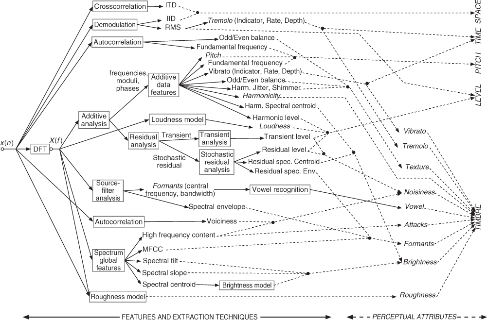
There are some relationships between low-level features and perceptual features, as some perceptual features are approximated by some low-level sound features. A non-exhaustive set of sound features [VZA06] shown in Figure 9.5 will contain various sound features that are commonly used for timbre space description (for instance based on MPEG-7 proposals [PMH00]) as well as features computed by perceptual models such as the ones extracted by the PsySound software [Cab99] in an offline (non-real-time) context: pitch, loudness, brightness, roughness, etc. Therefore, the wider the sound-feature set, the more chances we have to grasp the sound information along all perceptual attributes, with a consequent increase in information redundancy.
Figure 9.5 Example set of sound features that can be used as control parameters in adaptive effects [VZA06]. The arrow line types indicate the techniques used for extraction (left and plain lines) and the related perceptual attribute (right and dashed lines). Italic words refer to perceptual attributes. Figure reprinted with IEEE permission from [VZA06]
Acquisition Method
Various acquisition and computation methods can be used. A sound feature f(m) can be obtained directly, as is the sound amplitude by RMS. It can also be obtained indirectly, as the derivative:
9.1 ![]()
9.2 ![]()
with Ra the analysis increment step, fS the sampling rate. While instantaneous sound features provide information about acoustical or perceptual features, their derivatives inform about the evolution of such features. It can also be obtained indirectly as the integration, the absolute value, the mean of the standard deviation of another parameter. In this latter case, it can be seen as obtained through a given mapping. However, as soon as this new feature has a descriptive meaning, it can also be considered as a new feature.
Integration Time
Each parameter is computed and has a meaning only for a given time interval. Due to the time-frequency uncertainty (similar to the Heisenberg principle in quantum mechanics), no sound feature can be considered as really instantaneous, but rather is obtained from a certain number of sound samples, and is then quasi-instantaneous. This remark can also be expanded to samples themselves, as they represent the sound wave of a given time interval with a single value. We will then consider that quasi-instantaneous features correspond to parameters extracted from a 512 to 2048 samples of a signal sampled at 44.1 kHz, representing 12–46 ms. Mid-term sound features are features derived from the mean, the standard variance, the skewness or the kurtosis (i.e., the four first-order statistical moments) of N values of a parameter using a sliding window, or the beat, loudness. Long-term sound features are descriptors based on the signal description, and, for instance, relate to notes, presence/absence of acoustical effects such as vibrato, tremolo, flutter-tonguing. Very long-term sound features describe a whole musical excerpt in terms of a sound sequence as seen through music analysis: style, tonality, structure, etc.
The integration time is then related to sound segmentation and region attributes, on which sound feature statistics (mean, standard deviation) are useful. While sound features such as spectral centroid and fundamental frequency can be computed as (almost) instantaneous parameters, there are also sound descriptions that require longer-term estimation and processing. For instance, some loudness perceptual models account for time integration.
Moreover, one may want to segment a note into attack/decay/sustain/release and extract specific features for each section. One may also want to segment a musical excerpt into notes and silences, and then process differently each note, or each sequence of notes, depending on some criterion. This is the case for auto-tune (even though this is somewhat done on-the-fly), swing change (adaptive time-scaling with onset modification depending on the rhythm), etc. Such adaptive segmentation processes may use both low-level and/or high-level features. Note that even in the context of real-time implementation, sound features are not really instantaneous, as they often are computed with a block-by-block approach. Therefore, we need, when describing low-level and high-level features, to indicate their instantaneous and segmental aspects as well. Sound segmentation, which is a common resource in automatic speech-recognition systems, as well as in automatic music-transcription systems, score-following systems, etc., has a central place in ADAFX. Since the late 1990s, music segmentation applications [Ros98] started to use techniques originally developed in the context of speech segmentation [VM90], such as those based on pattern recognition or knowledge-based methodologies.
Type
We may consider at least two main types of sound descriptors: continuous and indicators. Indicators are parameters that can take a small and limited number of discrete values, for instance the presence of an acoustical effect (vibrato, tremolo, flutter-tonguing) or the identification of a sung vowel among a subset of five. Conversely, continuous features are features that can take any value in a given range, for instance the amplitude with RMS in the interval [0, 1] or the fundamental frequency in the interval [20, 20000] Hz. An intertwined case is the probability or pseudo probability that is continuous, but can also be used as an indicator as soon as it is coupled with a threshold. The voiciness computed from autocorrelation is such a feature, as it can indicate if the sound is harmonic/voicy or not depending on a continuous value in [0, 1] and a threshold around 0.8. By definition, indicators are higher-level features than continuous descriptors.
Causality
A sound feature can be computed either only from past samples, in which case it is a causal process, or from past and future samples, in which case it is an anti-causal process. For instance, when considering a time frame, the sound intensity computed by RMS, using the last frame sample as the reference time of the frame will make this computation causal (it can be obtained in real-time), whereas attributing this value to the frame central time will consider this as an anti-causal process. Only causal processing can be performed in real-time (with a latency depending on both the frame size and the computational time), thus limiting the possible real-time applications to the sound features available in real-time.
Time and Time-frequency Domains
A sound feature directly computed from the wave form uses a time-domain computation, whereas a sound feature computed from the Fourier transform of a time frame uses a frequency-domain computation. We will use this classification. While these six ways to look at sound features inform us about their properties and computation, the next sections will use the perceptual attribute described by the sound feature as a way to organize descriptions of various sound features. As proposed in Section 1.2.2 of Chapter 1, we now present sound features classified according to the perceptual attribute they relate to, namely: loudness, time, pitch, spatial hearing, and timbre.
9.2.2 Loudness-related Sound Features
Amplitude Envelope
One very important feature that can be used for adaptive effects is the amplitude envelope of a sound evolving with time. Even the modulation of a sound by the envelope of another sound is an effect by itself. But more generally the amplitude envelope can be used to control many variables of an effect. Applications of amplitude detection can be found in dynamics processing (see Chapter 4), but can also be integrated into many effects as an external control parameter.
Except for the fact that we want to write a signal as x(n) = amp(n) · sig(n), there is no unique definition of an amplitude envelope of a sound. The ear is devised in such a way that slow variations of amplitude (under 10 Hz) are considered as a time envelope while more rapid variations would be heard as a sound. This distinction between an envelope and a signal is known in electroacoustic music as the difference between a ‘shape’ and a ‘matter,’ two terms well developed by P. Schaeffer in his Traité des objets musicaux [Sch66].
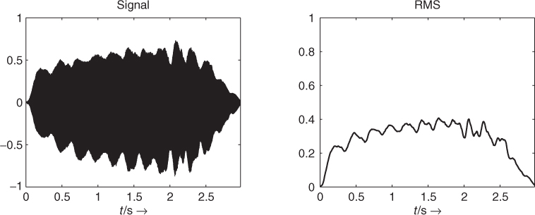
The RMS (root mean square) algorithm has been largely used in Chapter 4 as an amplitude detector based on filtering the squared input samples and taking the square root of the filter output. The RMS value is a good indication of the temporal variation of the energy of a sound, as shown in Figure 9.6. This filtering can also be performed by a FIR filter, and in this case can be inserted into an FFT/IFFT-based analysis-synthesis scheme for a digital audio effect. The FFT window can be considered a lowpass FIR filter, and one of the reasons for the crucial choice of window size for a short-time Fourier transform is found in the separation between shape and matter: if the window is too short, the envelope will follow rapid oscillations which should not be included. If the window is too large, the envelope will not take into account tremolos which should be included. The following M-file 9.1 calculates the amplitude envelope of a signal according to an RMS algorithm.
M-file 9.1 (UX_rms.m)
% Author: Verfaille, Arfib, Keiler, Zölzer
clear; clf
%----- USER DATA -----
[DAFx_in, FS] = wavread('x1.wav'),
hop = 256; % hop size between two FFTs
WLen = 1024; % length of the windows
w = hanningz(WLen);
%----- some initializations -----
WLen2 = WLen/2;
normW = norm(w,2);
pft = 1;
lf = floor((length(DAFx_in) - WLen)/hop);
feature_rms = zeros(lf,1);
tic
%===========================================
pin = 0;
pend = length(DAFx_in) - WLen;
while pin<pend
grain = DAFx_in(pin+1:pin+WLen).* w;
feature_rms(pft) = norm(grain,2) / normW;
pft = pft + 1;
pin = pin + hop;
end
% ===========================================
toc
subplot(2,2,1); plot(DAFx_in); axis([1 pend -1 1])
subplot(2,2,2); plot(feature_rms); axis([1 lf -1 1])
Figure 9.6 Signal and amplitude envelope (RMS value) of the signal.
When using a spectral model, one can separate the amplitude of the sinusoidal component and the amplitude of the residual component. The amplitude of the sinusoidal component is computed for a given frame m as the sum of the amplitude for all L harmonics given by
9.3 
with ai(m) the linear amplitude of the ith harmonic. It can also be expressed in dB as
9.4 
The amplitude of the residual component is the sum of the absolute values of the residual of one frame, and can also be computed according to
9.5 
where xR(n)is the residual sound, M is the block size, XR(k) is residual sound spectrum, and N the magnitude spectrum size.
Sound Energy
The instantaneous sound energy is the squared amplitude. It can either be derived from the wave form by
9.6 ![]()
from a time-frequency representation for the mth block by
9.7 
or also from a spectral representation by
9.8 
Loudness
There exist various computational models of loudness, starting from Zwicker's model [ZS65, Zwi77] to various improvements by Zwicker and Fastl [ZF99], Moore and Glasberg [MG96, MGB97], most of them being implemented in the Psysound32 [Cab99, Cab00]. Generally speaking, these models consider a critical band in the spectrum, onto which the energy is summed after accounting for frequency masking. More improved models also account for time integration and masking. Since the loudness of a sound depends on the sound level at which it is played, various different loudness curves can be obtained as control curves for adaptive effect control.
Tremolo Description
Using a sinusoidal model of the amplitude envelope, one can describe the time evolution of a tremolo in terms of rate or frequency (in Hz), amplitude or depth (in dB), and phase at the start. Those parameters can be used as sound features for other purposes. An example is the special sinusoidal model [MR04], when it is used for time-scaling of vibrato sounds, while preserving the vibrato attributes.
9.2.3 Time Features: Beat Detection and Tracking
A useful feature for controlling parameters of digital audio effects is the actual tempo or so-called beats-per-minute measure. In a live playing situation usually a drummer or conductor counts the tempo in by hitting his stick, which gives the first precise estimate for the beat. So the beat per minute is known from the very beginning. In a recording situation the first tracks are usually recorded with a so-called click track which is given by the recording system and everything is played in sync to that track. In both situations the beat is detected by simple means of listening and playing in sync to the beat. The beat signal can be used to control effect parameters, such as delay-time settings, speed of parameter modulation, gates for reverb and so on. A variety of beat-synced effects can be found in the Adrenalinn product. In the following, a robust and proven concept based on [BFC05, Fit04, Fit10] will be introduced which offers beat detection and tracking. The beat detection and tracking has a pre-processing stage which separates harmonic and percussive parts for further onset detection of harmonic and percussive signals. The harmonic/percussion separation is based on processing on the spectrogram, making use of median filtering across each frame in frequency direction and across each frequency bin in the time direction (see Figure 9.7).
Figure 9.7 Signal spectrogram, difference spectrogram, and time-domain signal and its beat indicators.
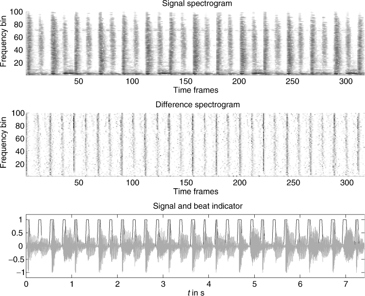
This separation technique is based on the idea that as a first approximation, broadband noise signals such as drums can be regarded as stable vertical ridges in a spectrogram. Therefore, the presence of narrow band signals, such as the harmonics from a pitched instrument, will result in an increase in energy within a bin over and above that due to the drum instrument, resulting in outliers in the spectrogram frame. These can be removed by the use of a median filter, thereby suppressing the harmonic information within the spectrogram frame. The median filtered frames are stored in a percussion enhanced spectrogram, denoted P(n, k). Similarly, the harmonics of pitched instruments can be regarded as stable horizontal ridges in a spectrogram. In this case, a sudden onset due to a drum or percussion instrument will result in a large increase in energy across time within a given frequency slice. This will again result in outliers in the evolution of the frequency slice with time, which can be removed by median filtering, thereby suppressing percussive events within the frequency bin. The median-filtered frequency slices are then stored in a harmonic-enhanced spectrogram H(n, k). However, as median filtering is a non-linear operation which introduces artifacts into the spectrogram, it is better to use the enhanced spectrograms obtained from median filtering to create masks to be applied to the original spectrogram. This can be done using a Wiener-filtering-based approach, which delivers the harmonic spectrogram
9.9 ![]()
and the percussive spectrogram
9.10![]()
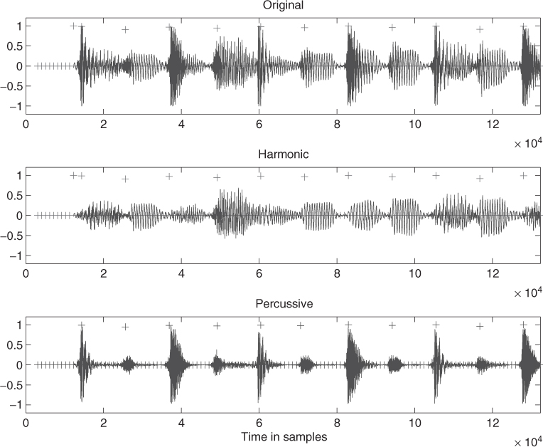
These spectrograms can then be inverted to the time domain by the inverse short-time Fourier transform. Beats are then detected by carrying out differentiation between successive frames X(n, k) − X(n − 1, k) and counting the number of frequency bins which have a positive energy change. This is a simple method for detecting the occurrence of a broadband noise signal such as a drum. As this method is not based on the amount of energy in the signal, it can be used to detect low-energy noise-based events. By setting a threshold of how many bins have to be positive before an event is considered to be detected, and by keeping only local maxima in this function, a beat detection function can be obtained. This is illustrated on both the original signal (spectrogram), as well as the separated harmonic and percussion signal (spectrogram) (see Figure 9.8). The following M-file 9.2 shows the harmonic/percussion separation. The code assumes odd length median filters with p as the power to which the separated spectrogram frames are raised when generating masks to be applied to the original spectrogram frame. The output of the percussive separation is then used to generate an onset detection function for use with beat-driven effects.
M-file 9.2 (HPseparation.m)
% Author: Derry FitzGerald
%----- user data -----
WLen =4096;
hopsize =1024;
lh =17; % length of the harmonic median filter
lp =17; % length of the percussive median filter
p =2;
w1 =hanning(WLen,'periodic'),
w2 =w1;
hlh =floor(lh/2)+1;
th =2500;
[DAFx_in, FS] =wavread('filename'),
L = length(DAFx_in);
DAFx_in = [zeros(WLen, 1); DAFx_in; ...
zeros(WLen-mod(L,hopsize),1)] / max(abs(DAFx_in));
DAFx_out1 = zeros(length(DAFx_in),1);
DAFx_out2 = zeros(length(DAFx_in),1);
%----- initialisations -----
grain = zeros(WLen,1);
buffer = zeros(WLen,lh);
buffercomplex = zeros(WLen,lh);
oldperframe = zeros(WLen,1);
onall = [];
onperc = [];
tic
%UUUUUUUUUUUUUUUUUUUUUUUUUUUUUUUUUUUUUUU
pin = 0;
pout = 0;
pend = length(DAFx_in)-WLen;
while pin<pend
grain = DAFx_in(pin+1:pin+WLen).* w1;
%===========================================
fc = fft(fftshift(grain));
fa = abs(fc);
% remove oldest frame from buffers and add
% current frame to buffers
buffercomplex(:,1:lh-1)=buffercomplex(:,2:end);
buffercomplex(:,lh)=fc;
buffer(:,1:lh-1)=buffer(:,2:end);
buffer(:,lh)=fa;
% do median filtering within frame to suppress harmonic instruments
Per = medfilt1(buffer(:,hlh),lp);
% do median filtering on buffer to suppress percussion instruments
Har = median(buffer,2);
% use these Percussion and Harmonic enhanced frames to generate masks
maskHar = (Har.∧p)./(Har.∧p + Per.∧p);
maskPer = (Per.∧p)./(Har.∧p + Per.∧p);
% apply masks to middle frame in buffer
% Note: this is the “current” frame from the point of view of the median
% filtering
curframe=buffercomplex(:,hlh);
perframe=curframe.*maskPer;
harframe=curframe.*maskHar;
grain1 = fftshift(real(ifft(perframe))).*w2;
grain2 = fftshift(real(ifft(harframe))).*w2;
% onset detection functions
% difference of frames
dall=buffer(:,hlh)-buffer(:,hlh-1);
dperc=abs(perframe)-oldperframe;
oall=sum(dall>0);
operc=sum(dperc>0);
onall = [onall oall];
onperc = [onperc operc];
oldperframe=abs(perframe);
%===========================================
DAFx_out1(pout+1:pout+WLen) = ...
DAFx_out1(pout+1:pout+WLen) + grain1;
DAFx_out2(pout+1:pout+WLen) = ...
DAFx_out2(pout+1:pout+WLen) + grain2;
pin = pin + hopsize;
pout = pout + hopsize;
end
%UUUUUUUUUUUUUUUUUUUUUUUUUUUUUUUUUUUUUUU
toc
% process onset detection function to get beats
[or,oc]=size(onall);
omin=min(onall);
% get peaks
v1 = (onall > [omin, onall(1:(oc-1))]);
% allow for greater-than-or-equal
v2 = (onall >= [onall(2:oc), omin]);
% simple Beat tracking function
omax = onall .* (onall > th).* v1 .* v2;
% now do the same for the percussion onset detection function
% process onset detection function to get beats
[opr,opc]=size(onperc);
opmin=min(onperc);
% get peaks
p1 = (onperc > [opmin, onperc(1:(opc-1))]);
% allow for greater-than-or-equal
p2 = (onperc >= [onperc(2:opc), opmin]);
% simple Beat tracking function
opmax = onperc .* (onperc > th).* p1 .* p2;
%----- listening and saving the output -----
DAFx_out1 = DAFx_out1((WLen + hopsize*(hlh-1)) ...
:length(DAFx_out1))/max(abs(DAFx_out1));
DAFx_out2 = DAFx_out2(WLen + (hopsize*(hlh-1)) ...
:length(DAFx_out2))/max(abs(DAFx_out2));
% soundsc(DAFx_out1, FS);
% soundsc(DAFx_out2, FS);
wavwrite(DAFx_out1, FS, 'ex-percussion.wav'),
wavwrite(DAFx_out2, FS, 'ex-harmonic.wav'),
Avoiding latency and improving the robustness of the detection function can be obtained by using high-order prediction approaches in frame and frequency direction [NZ08] compared to the simple one-frame prediction (difference). Several further features can be derived from such kinds of low-level beat detector [Fit04, UH03, SZST10].
Figure 9.8 Original signal with onset markers, harmonic signal with onset markers, and percussive signal with beat markers.
9.2.4 Pitch Extraction
The main task of pitch extraction is to estimate a fundamental frequency f0, which in musical terms is the pitch of a sound segment, and follow the fundamental frequency over the time. We can use this pitch information to control effects like time stretching and pitch shifting based on the PSOLA method, which is described in Chapter 6, but it also plays a major role in sound modeling with spectral models, which is treated extensively in Chapter 10. Moreover, the fundamental frequency can be used as a control parameter for a variety of audio effects based either on time-domain or on frequency-domain processing.
There is no definitive technique for pitch extraction and tracking, and only the bases of existing algorithms will be described here. We will consider pitch extraction both in the frequency domain and in the time domain. An overview and comparison of the presented algorithms can be found in [KZ10]. Most often an algorithm first looks for candidates of a pitch, then selects one and tries to improve the precision of the choice. After the calculation of pitch candidates post-processing, for example, pitch tracking has to be applied. During post-processing the estimation of the fundamental frequency from the pitch candidates can be improved by taking the frequency relationships between the detected candidates into account, which should ideally be multiples of the fundamental frequency.
FFT-based Approach
In this subsection we describe the calculation of pitch candidates from the FFT of a signal segment where the phase information is used. This approach is similar to the technique used in the phase vocoder, see Section 7.3. The main structure of the algorithm is depicted in Figure 9.9, where a segment of length N is extracted every R samples and then applied to FFTs.
Figure 9.9 FFT-based pitch estimation structure with phase evaluation.
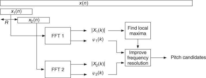
Considering the calculation of an N-point FFT, the frequency resolution of the FFT is
9.11 ![]()
with the sampling frequency fS = 1/TS. From the input signal x(n) we use a block
9.12 ![]()
of N samples. After applying an appropriate window, the FFT yields X1(k) with k = 0, …, N − 1. At the FFT index k0 a local maximum of the FFT magnitude |X1(k)| is detected. From this FFT maximum, the initial estimate of the fundamental frequency is
9.13 ![]()
The corresponding normalized frequency is
9.14 ![]()
To improve the frequency resolution, the phase information can be used, since for a harmonic signal xh(n) = cos(Ω0n + φ0) = cos(ϕ(n)) the fundamental frequency can be computed by the derivative
9.15 ![]()
The derivative can be approximated by computing the phases of two FFTs separated by a hop size of R samples leading to
9.16 ![]()
where Δϕ is the phase difference between the two FFTs evaluated at the FFT index k0. The second FFT of the signal segment
9.17 ![]()
leads to X2(k). For the two FFTs, the phases at frequency ![]() are given by
are given by
9.18 ![]()
9.19 ![]()
Both phases φ1 and φ2 are obtained in the range [−π, π]. We now calculate an ‘unwrapped’ φ2 value corresponding to the value of an instantaneous phase, see also Section 7.3.5 and Figure 7.17. Assuming that the signal contains a harmonic component with a frequency ![]() , the expected target phase after a hop size of R samples is
, the expected target phase after a hop size of R samples is
9.20 ![]()
The phase error between the unwrapped value φ2 and the target phase can be computed by
9.21 ![]()
The function ‘princarg’ computes the principal phase argument in the range [ − π, π]. It is assumed that the unwrapped phase differs from the target phase by a maximum of π. The unwrapped phase is obtained by
9.22 ![]()
The final estimate of the fundamental frequency is then obtained by
9.23 ![]()
Normally we assume that the first pitch estimation ![]() differs from the fundamental frequency by a maximum of Δf/2. Thus the maximum amount for the absolute value of the phase error φ2err is
differs from the fundamental frequency by a maximum of Δf/2. Thus the maximum amount for the absolute value of the phase error φ2err is
9.24 ![]()
We should accept phase errors with slightly higher values to have some tolerance in the pitch estimation.
One simple example of an ideal sine wave at a fundamental frequency of 420 Hz at fS = 44.1 kHz analyzed with the FFT length N = 1024 using a Hanning window and hop size R = 1 leads to the following results: k0 = 10, ![]() , φ1/π = − 0.2474, φ2t/π = − 0.2278, φ2/π = − 0.2283,
, φ1/π = − 0.2474, φ2t/π = − 0.2278, φ2/π = − 0.2283, ![]() . Thus the original sine frequency is almost ideally recovered by the described algorithm.
. Thus the original sine frequency is almost ideally recovered by the described algorithm.
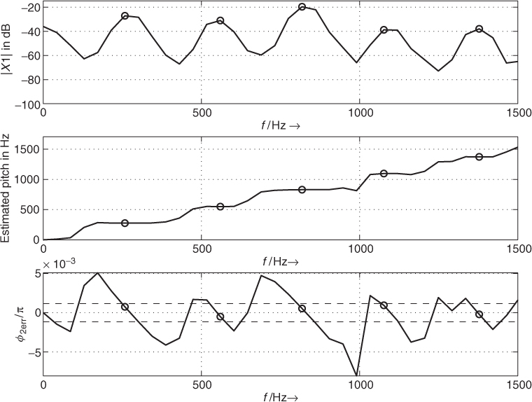
Figure 9.10 shows an example of the described algorithm applied to a short signal of the female utterance ‘la’ analyzed at an FFT length N = 1024. The top plot shows the FFT magnitude, the middle plot the estimated pitch, and the bottom plot the phase error φ2err for frequencies up to 1500 Hz. For this example the frequency evaluation is performed for all FFT bins and not only for those with detected magnitude maxima. The circles show the positions of detected maxima in the FFT magnitude. The dashed lines in the bottom plot show the used threshold for the phase error. In this example the first maximum is detected at FFT index k0 = 6, the corresponding bin frequency is 258.40 Hz, and the corrected pitch frequency is 274.99 Hz. Please notice that in this case the magnitude of the third harmonic (at appr. 820 Hz) has a greater value than the magnitude of the fundamental frequency.
Figure 9.10 Example of pitch estimation of speech signal ‘la.’
M-file 9.3 presents a MATLAB® implementation to calculate the pitch candidates from a block of the input signal.
M-file 9.3 (find_pitch_fft.m)
function [FFTidx, Fp_est, Fp_corr] = ...
find_pitch_fft(x, win, Nfft, Fs, R, fmin, fmax, thres)
% [DAFXbook, 2nd ed., chapter 9]
%===== This function finds pitch candidates
%
% Inputs:
% x: input signal of length Nfft+R
% win: window for the FFT
% Nfft: FFT length
% Fs: sampling frequency
% R: FFT hop size
% fmin, fmax: minumum/ maximum pitch freqs to be detected
% thres: %omit maxima more than thres dB below the main peak
% Outputs:
% FFTidx: FFT indices
% Fp_est: FFT bin frequencies
% Fp_corr: corrected frequencies
FFTidx = [];
Fp_est = [];
Fp_corr = [];
dt = R/Fs; % time diff between FFTs
df = Fs/Nfft; % freq resolution
kp_min = round(fmin/df);
kp_max = round(fmax/df);
x1 = x(1:Nfft); % 1st block
x2 = x((1:Nfft)+R); % 2nd block with hop size R
[X1, Phi1] = fftdb(x1.*win,Nfft);
[X2, Phi2] = fftdb(x2.*win,Nfft);
X1 = X1(1:kp_max+1);
Phi1 = Phi1(1:kp_max+1);
X2 = X2(1:kp_max+1);
Phi2 = Phi2(1:kp_max+1);
idx = find_loc_max(X1);
Max = max(X1(idx));
ii = find(X1(idx)-Max>-thres);
%----- omit maxima more than thres dB below the main peak -----
idx = idx(ii);
Nidx = length(idx); % number of detected maxima
maxerr = R/Nfft; % max phase diff error/pi
% (pitch max. 0.5 bins wrong)
maxerr = maxerr*1.2; % some tolerance
for ii=1:Nidx
k = idx(ii) - 1; % FFT bin with maximum
phi1 = Phi1(k+1); % phase of x1 in [-pi,pi]
phi2_t = phi1 + 2*pi/Nfft*k*R; % expected target phase
% after hop size R
phi2 = Phi2(k+1); % phase of x2 in [-pi,pi]
phi2_err = princarg(phi2-phi2_t);
phi2_unwrap = phi2_t+phi2_err;
dphi = phi2_unwrap - phi1; % phase diff
if (k>kp_min) & (abs(phi2_err)/pi<maxerr)
Fp_corr = [Fp_corr; dphi/(2*pi*dt)];
FFTidx = [FFTidx; k];
Fp_est = [Fp_est; k*df];
end
end
In addition to the algorithm described, the magnitude values of the detected FFT maxima are checked. In the given code those maxima are omitted whose FFT magnitudes are more than thres dB below the global maximum. Typical values for the parameter thres lie in the range from 30 to 50. The function princarg is given in Figure 7.17. The following function fftdb (see M-file 9.4) returns the FFT magnitude in a dB scale and the phase.
M-file 9.4 (fftdb.m)
function [H, phi] = fftdb(x, Nfft)
% [DAFXbook, 2nd ed., chapter 9]
%==== This function discards values in FFT bins for which magnitude >Â thresh
if nargin<2
Nfft = length(x);
end
F = fft(x,Nfft);
F = F(1:Nfft/2+1); % f=0,..,Fs/2
phi = angle(F); % phase in [-pi,pi]
F = abs(F)/Nfft*2; % normalize to FFT length
%----- return -100 db for F==0 to avoid “log of zero” warnings -----
H = -100*ones(size(F));
idx = find(F∼=0);
H(idx) = 20*log10(F(idx)); % non-zero values in dB
The following function find_loc_max (see M-file 9.5) searches for local maxima using the derivative.
M-file 9.5 (find_loc_max.m)
function [idx, idx0] = find_loc_max(x)
% [DAFXbook, 2nd ed., chapter 9]
%===== This function finds local maxima in vector x
% Inputs:
% x: any vector
% Outputs:
% idx : positions of local max.
% idx0: positions of local max. with 2 identical values
% if only 1 return value: positions of all maxima
N = length(x);
dx = diff(x); % derivation
% to find sign changes from + to -
dx1 = dx(2:N-1);
dx2 = dx(1:N-2);
prod = dx1.*dx2;
idx1 = find(prod<0); % sign change in dx1
idx2 = find(dx1(idx1)<0); % only change from + to -
idx = idx1(idx2)+1; % positions of single maxima
%----- zeros in dx? => maxima with 2 identical values -----
idx3 = find(dx==0);
idx4 = find(x(idx3)>0); % only maxima
idx0 = idx3(idx4);
%----- positions of double maxima, same values at idx3(idx4)+1 -----
if nargout==1 % output 1 vector
% with positions of all maxima
idx = sort([idx,idx0]); % (for double max. only 1st position)
end
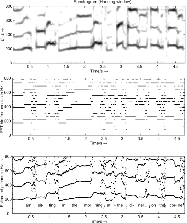
Now we present an example where the algorithm is applied to a signal segment of Suzanne Vega's ‘Tom's Diner.’ Figure 9.11 shows time-frequency representations of the analysis results. The top plot shows the spectrogram of the signal. The middle plot shows the FFT bin frequencies of detected pitch candidates while the bottom plot shows the corrected frequency values. In the bottom plot the text of the sung words is also shown. In all plots frequencies up to 800 Hz are shown. For the spectrogram an FFT length of 4096 points is used. The pitch-estimation algorithm is performed with an FFT length of 1024 points. This example shows that the melody of the sound can be recognized in the bottom plot of Figure 9.11. The applied algorithm improves the frequency resolution of the FFT shown in the middle plot. To choose the correct pitch among the detected candidates some post-processing is required. Other methods to improve the frequency resolution of the FFT are described in [Can98, DM00, Mar00, Mar98, AKZ99] and in Chapter 10.
Figure 9.11 Time/frequency planes for pitch estimation example of an excerpt from Suzanne Vega's ‘Tom's Diner.’ Top: spectrogram, middle: FFT bin frequencies of pitch candidates, bottom: corrected frequency values of pitch candidates.
M-file 9.6 demonstrates a pitch-tracking algorithm in a block-based implementation.
M-file 9.6 (Pitch_Tracker_FFT_Main.m)
% Pitch_Tracker_FFT_Main.m [DAFXbook, 2nd ed., chapter 9]
%===== This function demonstrates a pitch tracking algorithm
%===== in a block-based implementation
%----- initializations -----
fname='Toms_diner';
n0=2000; %start index
n1=210000;
Nfft=1024;
R=1; % FFT hop size for pitch estimation
K=200; % hop size for time resolution of pitch estimation
thres=50; % threshold for FFT maxima
% checked pitch range in Hz:
fmin=50;
fmax=800;
p_fac_thres=1.05; % threshold for voiced detection
% deviation of pitch from mean value
win=hanning(Nfft)';% window for FFT
Nx=n1-n0+1+R; % signal length
blocks=floor(Nx/K);
Nx=(blocks-1)*K+Nfft+R;
n1=n0+Nx; % new end index
[X,Fs]=wavread(fname,[n0,n1]);
X=X(:,1)';
%----- pitch extraction per block -----
pitches=zeros(1,blocks);
for b=1:blocks
x=X((b-1)*K+1+(1:Nfft+R));
[FFTidx, F0_est, F0_corr]= ...
find_pitch_fft(x,win,Nfft,Fs,R,fmin,fmax,thres);
if ∼isempty(F0_corr)
pitches(b)=F0_corr(1); % take candidate with lowest pitch
else
pitches(b)=0;
end
end
%----- post-processing -----
L=9; % odd number of blocks for mean calculation
D=(L-1)/2; % delay
h=ones(1,L)./L; % impulse response for mean calculation
%----- mirror beginning and end for “non-causal” filtering -----
p=[pitches(D+1:-1:2),pitches,pitches(blocks-1:-1:blocks-D)];
y=conv(p,h); % length: blocks+2D+2D
pm=y((1:blocks)+2*D); % cut result
Fac=zeros(1,blocks);
idx=find(pm∼=0); % don't divide by zero
Fac(idx)=pitches(idx)./pm(idx);
ii=find(Fac<1 & Fac∼=0);
Fac(ii)=1./Fac(ii); % all non-zero elements are now > 1
%----- voiced/unvoiced detection -----
voiced=Fac∼=0 & Fac<p_fac_thres;
T=40; % time in ms for segment lengths
M=round(T/1000*Fs/K); % min. number of consecutive blocks
[V,p2]=segmentation(voiced, M, pitches);
p2=V.*p2; % set pitches to zero for unvoiced
%----- plotting and drawing figure -----
figure(1),clf,
time=(0:blocks-1)*K+1; % start sample of blocks
time=time/Fs; % time in seconds
t=(0:length(X)-1)/Fs; % time in sec for original
subplot(211)
plot(t,X),title('original x(n)')
axis([0 max([t,time]) -1.1*max(abs(X)) 1.1*max(abs(X))])
subplot(212)
idx=find(p2∼=0);
plot_split(idx,time, p2),title('pitch in Hz'),
xlabel('time/s ightarrow'),
axis([0 max([t,time]) .9*min(p2(idx)) 1.1*max(p2(idx))])
In the above implementation the post-processing is performed by choosing the lowest pitch candidate in each block. Then the mean pitch of surrounding blocks is computed and compared to the detected pitch. If the deviation from the mean value is higher than a given threshold, this block is considered as ‘unvoiced.’ Finally a segmentation is performed to get a minimum number of consecutive blocks that are voiced/unvoiced (to avoid very short segments). M-file 9.7 presents an implementation for the segmentation.
M-file 9.7 (segmentation.m)
function [V,pitches2] = segmentation(voiced, M, pitches)
% function [V,pitches2] = segmentation(voiced, M, pitches)
% [DAFXbook, 2nd ed., chapter 9]
%===== This function implements the pitch segmentation
%
% Inputs:
% voiced: original voiced/unvoiced detection
% M: min. number of consecutive blocks with same voiced flag
% pitches: original pitches
% Outputs:
% V: changed voiced flag
% pitches2: changed pitches
blocks=length(voiced); % get number of blocks
pitches2=pitches;
V=voiced;
Nv=length(V);
%%%%%%%%%%% step1: eliminate too short voiced segments:
V(Nv+1)=∼V(Nv); % change at end to get length of last segment
dv=[0, diff(V)]; % derivative
idx=find(dv∼=0); % changes in voiced
di=[idx(1)-1,diff(idx)]; % segment lengths
v0=V(1); % status of 1st segment
k0=1;
ii=1; % counter for segments, idx(ii)-1 is end of segment
if v0==0
k0=idx(1); % start of voiced
ii=ii+1; % first change voiced to unvoiced
end
while ii<=length(idx);
L=di(ii);
k1=idx(ii)-1; % end of voiced segment
if L<M
V(k0:k1)=zeros(1,k1-k0+1);
end
if ii<length(idx)
k0=idx(ii+1); % start of next voiced segment
end
ii=ii+2;
end
%%%%%%%%%%% step2: eliminate too short unvoiced segments:
V(Nv+1)=∼V(Nv); % one more change at end
dv=[0, diff(V)];
idx=find(dv∼=0); % changes in voiced
di=[idx(1)-1,diff(idx)]; % segment lengths
if length(idx)>1 % changes in V
v0=V(1); % status of 1st segment
k0=1;
ii=1; % counter for segments, idx(ii)-1 is end of segment
if v0==0
k0=idx(2); % start of unvoiced
ii=ii+2; % first change unvoiced to voiced
end
while ii<=length(idx);
L=di(ii);
k1=idx(ii)-1; % end of unvoiced segment
if L<M
if k1<blocks % NOT last unvoiced segment
V(k0:k1)=ones(1,k1-k0+1);
% linear pitch interpolation:
p0=pitches(k0-1);
p1=pitches(k1+1);
N=k1-k0+1;
pitches2(k0:k1)=(1:N)*(p1-p0)/(N+1)+p0;
end
end
if ii<length(idx)
k0=idx(ii+1); % start of next unvoiced segment
end
ii=ii+2;
end
end
V=V(1:Nv); % cut last element
The plot_split function is given by M-file 9.8.
M-file 9.8 (plot_split.m)
function plot_split(idx, t, x)
% function plot_split(idx, t, x) [DAFXbook, 2nd ed., chapter 9]
%===== This function plots the segmented pitch curve
% Inputs:
% idx: vector with positions of vector x to be plotted
% t: time indexes
% x is segmented into parts
di=diff(idx);
L=length(di);
n0=1;
pos_di=find(di>1);
ii=1; % counter for pos_di
hold off
while ii<=length(pos_di) %n0<=length(x)
n1=pos_di(ii);
plot(t(idx(n0:n1)),x(idx(n0:n1)))
hold on
n0=n1+1;
ii=ii+1;
end
n1=length(idx);
plot(t(idx(n0:n1)),x(idx(n0:n1)))
hold off
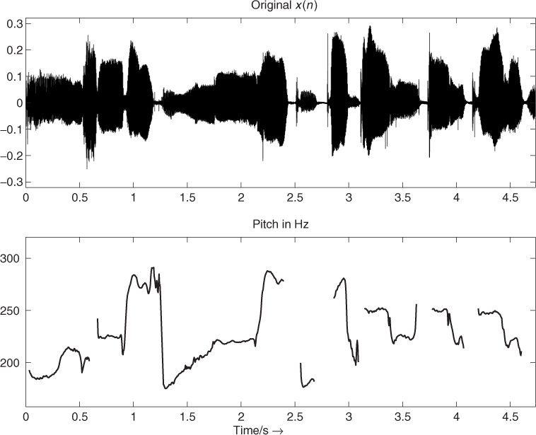
The result of the pitch-tracking algorithm is illustrated in Figure 9.12. The bottom plot shows the pitch over time calculated using the block-based FFT approach.
Figure 9.12 Pitch over time from the FFT with phase vocoder approach for a signal segment of Suzanne Vega's ‘Tom's Diner.’
Any FFT-based pitch estimator can be improved by detecting the harmonic structure of the sound. If the harmonics of the fundamental frequency are detected, the greatest common divisor of these harmonic frequencies can be used in the estimation of the fundamental frequency [O'S00, p. 220]. M.R. Schroeder mentions for speech processing in [Sch99, p. 65], ‘the pitch problem was finally laid to rest with the invention of cepstrum pitch detectors’ [Nol64]. The cepstrum technique allows the estimation of the pitch period directly from the cepstrum sequence c(n). Schroeder also suggested a ‘harmonic product spectrum’ [Sch68] to improve the fundamental frequency estimation, which sometimes outperforms the cepstrum method [Sch99, p. 65]. A further improvement of the pitch estimates can be achieved by applying a peak-continuation algorithm to the detected pitches of adjacent frames, which is described in Chapter 10.
General Remarks on Time-domain Pitch Extraction
In the time domain the task of pitch extraction leads us to find the corresponding pitch period. The pitch period is the time duration of one period. With the fundamental frequency f0 (to be detected) the pitch period is given by
9.25 ![]()
For a discrete-time signal sampled at ![]() we have to find the pitch lag M, which is the number of samples in one period. The pitch period is T0 = M · TS, which leads to
we have to find the pitch lag M, which is the number of samples in one period. The pitch period is T0 = M · TS, which leads to
Since only integer-valued pitch lags can be detected, we have a certain frequency resolution in detecting the fundamental frequency dependent on f0 and fS. Now we are assuming the case of ![]() where
where ![]() is the detected integer pitch lag. The detected fundamental frequency is
is the detected integer pitch lag. The detected fundamental frequency is ![]() instead of the exact pitch
instead of the exact pitch ![]() . The frequency error factor is in this case
. The frequency error factor is in this case
9.27 ![]()
With the halftone factor ![]() and setting
and setting ![]() , the frequency error in halftones is
, the frequency error in halftones is
9.28 ![]()
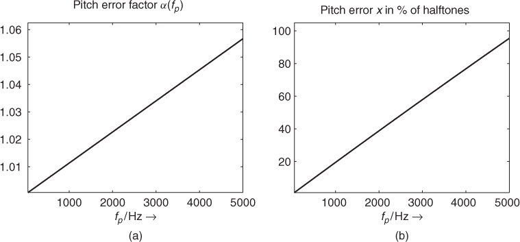
Figure 9.13 shows the frequency error both as factor α(f0) and as percentage of halftones for pitches in the range from 50 to 5000 Hz at the sampling frequency fS = 44.1 kHz. The maximum frequency error is approximately 6%, or one halftone, for pitches up to 5000 Hz. For a fundamental frequency of 1000 Hz the frequency error is only 20% of a halftone which is reasonably accurate precision.
Figure 9.13 Resolution of time-domain pitch detection at fS = 44.1 kHz, (a) frequency error factor, (b) pitch error in percentage of a halftone.
Normally the pitch estimation in the time domain is performed in three steps [O'S00, p. 218]:
1. Segmentation of the input signal into overlapping blocks and pre-processing of each block, for example lowpass filtering (see segmentation shown in Figure 9.9).
2. Basic pitch estimation algorithm applied to the pre-processed block.
3. Post-processing for an error correction of the pitch estimates and smoothing of pitch trajectories.
Auto-correlation and LPC
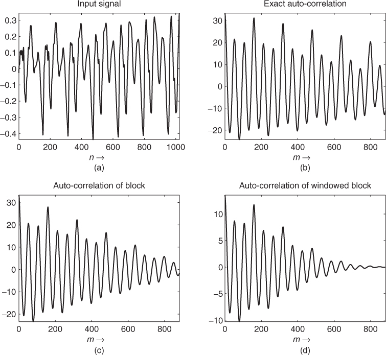
The auto-correlation sequence can also be used to detect the pitch period of a signal segment. First, we present different definitions of autocorrelation sequences:
- Using one block
- Using one windowed block
9.30
with u(n) = x(n) · w(n) (window function w(n))
- and Using the exact signal, thus using samples preceding the considered block
Notice, that in the definitions given by (9.29)–(9.31) no normalization to the block length N is applied.
Figure 9.14 shows the three different auto-correlation sequences for an excerpt of the speech signal “la.” Here the same input signal is used as in Figure 9.10. In this example the pitch lag corresponding to the fundamental frequency is M = 160 samples, and thus at the third maximum of the auto-correlation. Normally we expect the first maximum in the auto-correlation at the pitch lag. But sometimes, as in this example, the first maximum in the auto-correlation function is not at this position. In general, the auto-correlation has maxima at the pitch lag M and at its multiples, since, for a periodic signal, the same correlation occurs if comparing the signal with the same signal delayed by multiples of the pitch period. Since, in the example of Figures 9.10 and 9.14, the third harmonic is more dominant than the fundamental frequency, the first maximum in the auto-correlation is located at M/3. Conversely there can be a higher peak in the auto-correlation after the true pitch period.
Figure 9.14 Comparison between different autocorrelation computations for speech signal ‘la.’: (a) input block x(n), (b) exact auto-correlation ![]() , (c) standard auto-correlation rxx(m) using block, (d) standard auto-correlation rxx(m) using windowed block.
, (c) standard auto-correlation rxx(m) using block, (d) standard auto-correlation rxx(m) using windowed block.
Often the prediction error of an LPC analysis contains peaks spaced by the pitch period, see Figure 8.9. Thus it might be promising to try to estimate the pitch period from the prediction error instead of using the original signal. The SIFT algorithm [Mar72], which has been developed for voice, is based on removing the spectral envelope by inverse filtering in a linear prediction scheme. But in some cases it is not possible to estimate the pitch period from the prediction error, because the linear prediction has removed all pitch redundancies from the signal. Figure 9.15 compares two excerpts of a speech signal where the input block (top) and the auto-correlations of both the input signal (middle) and the prediction error (bottom) are shown. An LPC analysis of order p = 8 using the auto-correlation method has been applied.
Figure 9.15 Auto-correlation sequences for input signal and prediction error for two excerpts of the speech signal ‘la.’ Input signals (a, d), auto-correlation of input (b, e), auto-correlation of prediction error (c, f).
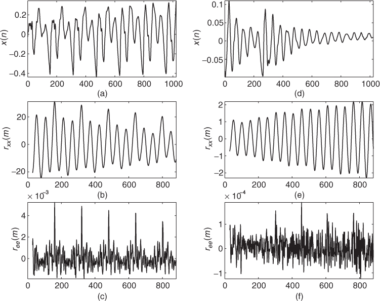
For the example presented in subplots (a)–(c) the pitch period can be well detected in the auto-correlation of the prediction error (same excerpt as in Figures 9.10 and 9.14). For the other excerpt presented in subplots (d)–(f) it is not possible to detect the pitch in the auto-correlation of the prediction error while the auto-correlation of the input signal has a local maximum at the correct pitch period. Notice that in the plots of the auto-correlation sequences only time-lag ranges from 29 to 882 are shown. This corresponds to pitch frequencies from 1500 down to 50 Hz at sampling frequency 44.1 kHz.
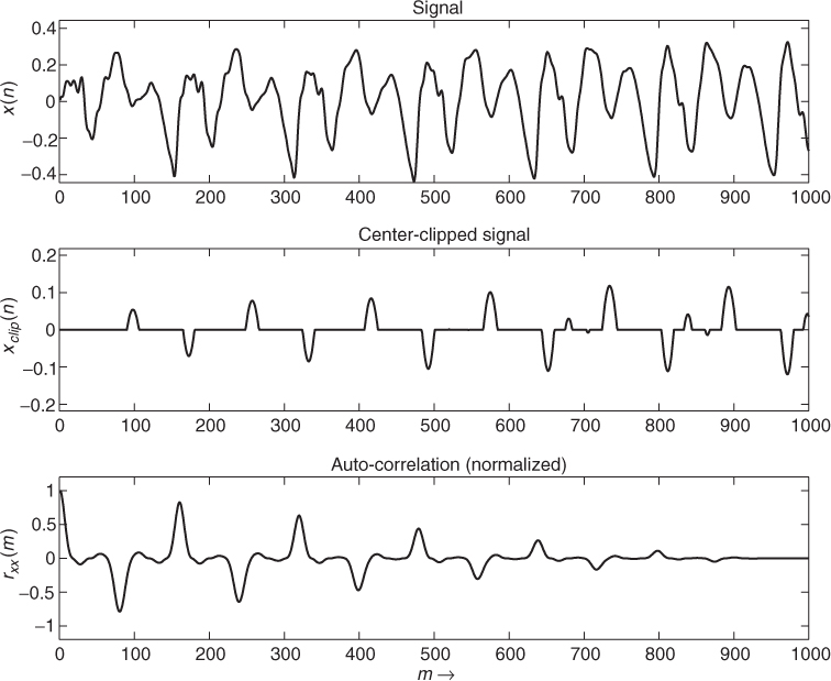
Another time-domain method for the extraction of the fundamental frequency is based on ‘center clipping’ the input signal and subsequent auto-correlation analysis [Son68]. First, the input signal is bandlimited by a lowpass filter. If the filter output signal exceeds a certain threshold ±c the operation ![]() is performed, otherwise
is performed, otherwise ![]() [RS78, Son68]. The result of this pre-processing is illustrated in Figure 9.16. The auto-correlation sequence rxx(m) of the center-clipped signal
[RS78, Son68]. The result of this pre-processing is illustrated in Figure 9.16. The auto-correlation sequence rxx(m) of the center-clipped signal ![]() shows a strong positive peak at the time lag of the pitch period.
shows a strong positive peak at the time lag of the pitch period.
Figure 9.16 Center clipping and subsequent auto-correlation analysis: input signal, lowpass filtered, and center-clipped signal (notice the time delay) and auto-correlation.
Narrowed Correlation: The YIN Algorithm
Another way to determine the periodicity of a signal is to calculate the sum of differences of a time frame with its shifted version analogous to the ACF. The average magnitude difference function (AMDF) [RSC+74] is defined as
9.32 
The function properties are similar to the ACF, but the AMDF shows dips at the lags of high correlation instead of peaks like the ACF does. De Cheveigné [dCK02] defined the difference function as sum of squared differences
9.33 
The ACF and the difference function are both sensitive to amplitude changes of the time signal. An increasing amplitude of the time signal leads to higher peaks at later lags for the ACF and lower dips for the difference function respectively. To avoid this a cumulative normalization is applied to average the current lag value with the previous values. The result is the normalized mean difference function (NMDF) defined as
9.34 
The NMDF starts at a value of 1 and drops below 1 only where the current lag value is below the average of all previous lags. This allows one to define a threshold, which a local minimum ![]() has to fall below in order to consider it as a valid pitch candidate (see figure 9.17). To increase the frequency resolution of the YIN algorithm the local minima of
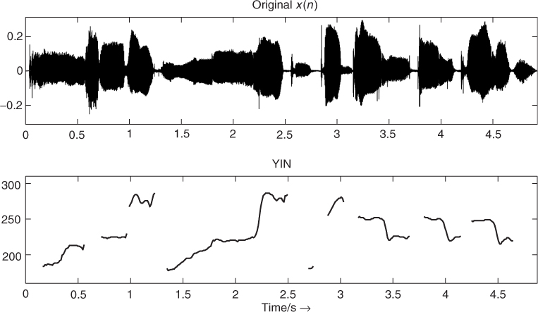
has to fall below in order to consider it as a valid pitch candidate (see figure 9.17). To increase the frequency resolution of the YIN algorithm the local minima of ![]() can be refined by parabolic interpolation with their neighboring lag values. The minimum of the parabola is used as the refined lag value. The result of the presented pitch-tracking algorithm is illustrated in Figure 9.18. The bottom plot shows the pitch over time calculated using the YIN algorithm.
can be refined by parabolic interpolation with their neighboring lag values. The minimum of the parabola is used as the refined lag value. The result of the presented pitch-tracking algorithm is illustrated in Figure 9.18. The bottom plot shows the pitch over time calculated using the YIN algorithm.
M-file 9.9 (yinDAFX.m)
function pitch = yinDAFX(x,fs,f0min,hop)
% function pitch = yinDAFX(x,fs,f0min,hop)
% Author: Adrian v.d. Knesebeck
% determines the pitches of the input signal x at a given hop size
%
% input:
% x input signal
% fs sampling frequency
% f0min minimum detectable pitch
% hop hop size
%
% output:
% pitch pitch frequencies in Hz at the given hop size
% initialization
yinTolerance = 0.22;
taumax = round(1/f0min*fs);
yinLen = 1024;
k = 0;
% frame processing
for i = 1:hop:(length(x)-(yinLen+taumax))
k=k+1;
xframe = x(i:i+(yinLen+taumax));
yinTemp = zeros(1,taumax);
% calculate the square differences
for tau=1:taumax
for j=1:yinLen
yinTemp(tau) = yinTemp(tau) + (xframe(j) - xframe(j+tau))∧2;
end
end
% calculate cumulated normalization
tmp = 0;
yinTemp(1) = 1;
for tau=2:taumax
tmp = tmp + yinTemp(tau);
yinTemp(tau) = yinTemp(tau) *(tau/tmp);
end
% determine lowest pitch
tau=1;
while(tau<taumax)
if(yinTemp(tau) < yinTolerance)
% search turning point
while (yinTemp(tau+1) < yinTemp(tau))
tau = tau+1;
end
pitch(k) = fs/tau;
break
else
tau = tau+1;
end
% if no pitch detected
pitch(k) = 0;
end
end
end
Figure 9.17 YIN algorithm: normalized mean difference function (NDMF) for a signal segment of Suzanne Vega's ‘Tom's Diner.’
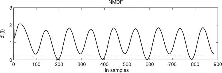
Figure 9.18 Pitch over time from the YIN algorithm for a signal segment of Suzanne Vega's ‘Tom's Diner.’
Long-term Prediction (LTP)
A further method of estimating the fundamental frequency is based on long-term prediction. A common approach to remove pitch-period redundancies from a signal is to use a short FIR prediction filter after a delay line of M samples, where M is the pitch lag [KA90]. Thus the long-term prediction error or residual is given by
9.35 
where the order q + 1 is normally in the range {1, 2, 3} [KA90]. Considering the case of a one-tap filter, the residual simplifies to
which is shown in Figure 9.19.
Figure 9.19 Long-term prediction with a one-tap filter.
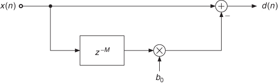
For minimizing the energy of d(n) over one block of length N we set the derivative with respect to b0 to zero. This leads to the optimal filter coefficient
9.37 ![]()
with ![]() as defined in (9.31) and
as defined in (9.31) and
9.38 
which is the energy of a block delayed by m samples. Setting this solution into (9.36) leads to the error energy
9.39 
dependent on M with
Figure 9.20 shows an example where the input signal shown in Figure 9.15(a) is used. The top plot shows the exact autocorrelation ![]() , the middle plot shows the normalized autocorrelation rxx,norm(m), and the bottom plot shows the LTP coefficient b0(m) dependent on the lag m.
, the middle plot shows the normalized autocorrelation rxx,norm(m), and the bottom plot shows the LTP coefficient b0(m) dependent on the lag m.
Figure 9.20 Auto-correlation, normalized auto-correlation and LTP coefficient dependent on lag m for excerpt from the speech signal ‘la.’ The circles show the pitch lag candidates, the dashed lines the accepted b0 values.
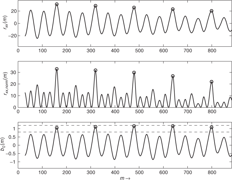
In rxx,norm(m) the lag m = M has to be found where rxx,norm(m) is maximized to minimize the residual energy. Considering one block of length N, the numerator of (9.40) is the squared auto-correlation, while the denominator is the energy of the block delayed by M samples. The function rxx,norm(m) therefore represents a kind of normalized auto-correlation sequence with only positive values. If used for the detection of the pitch period, rxx,norm(m) does not need to have a global maximum at m = M, but it is expected to have a local maximum at that position.
To find candidates of the pitch lag M, first local maxima in rxx,norm(m) are searched. In a second step, from these maxima only those ones are considered where the auto-correlation ![]() is positive valued. The function rxx,norm(m) also has maxima at positions where
is positive valued. The function rxx,norm(m) also has maxima at positions where ![]() has minima. In a third step the b0(m) values are considered. The value of the coefficient b0 is close to one for voiced sounds and close to zero for noise-like sounds [JN84, p. 315]. Thus the value of b0 can serve as a quality check for the estimate of the computed pitch lag.
has minima. In a third step the b0(m) values are considered. The value of the coefficient b0 is close to one for voiced sounds and close to zero for noise-like sounds [JN84, p. 315]. Thus the value of b0 can serve as a quality check for the estimate of the computed pitch lag.
In the example in Figure 9.20, b0 values in the range 0.8, … 1.2 are accepted. This range is shown by the dashed lines in the bottom plot. The circles represent the positions of pitch-lag candidates. Thus, at these positions rxx,norm(m) has a local maximum, ![]() is positive valued, and b0(m) lies in the described range. In this example, the first pitch lag candidate corresponds to the pitch of the sound segment.
is positive valued, and b0(m) lies in the described range. In this example, the first pitch lag candidate corresponds to the pitch of the sound segment.
The described algorithm for the computation of pitch-lag candidates from a signal block is implemented by the following M-file 9.10.
M-file 9.10 (find_pitch_ltp.m)
function [M,Fp] = find_pitch_ltp(xp, lmin, lmax, Nblock, Fs, b0_thres)
% function [M,Fp] = find_pitch_ltp(xp, lmin, lmax, Nblock, Fs, b0_thres)
% [DAFXbook, 2nd ed., chapter 9]
%===== This function computes the pitch lag candidates from a signal block
%
% Inputs:
% xp : input block including lmax pre-samples
% for correct autocorrelation
% lmin : min. checked pitch lag
% lmax : max. checked pitch lag
% Nblock : block length without pre-samples
% Fs : sampling freq.
% b0_thres: max b0 deviation from 1
%
% Outputs:
% M: pitch lags
% Fp: pitch frequencies
lags = lmin:lmax; % tested lag range
Nlag = length(lags); % no. of lags
[rxx_norm, rxx, rxx0] = xcorr_norm(xp, lmin, lmax, Nblock);
%----- calc. autocorr sequences -----
B0 = rxx./rxx0; % LTP coeffs for all lags
idx = find_loc_max(rxx_norm);
i = find(rxx(idx)>0); % only max. where r_xx>0
idx = idx(i); % indices of maxima candidates
i = find(abs(B0(idx)-1)<b0_thres);
%----- only max. where LTP coeff is close to 1 -----
idx = idx(i); % indices of maxima candidates
%----- vectors for all pitch candidates: -----
M = lags(idx);
M = M(:); % pitch lags
Fp = Fs./M;
Fp = Fp(:); % pitch freqs
The function find_loc_max is given in Section 9.2.4. The function xcorr_norm to compute the auto-correlation sequences is given by M-file 9.11.
M-file 9.11 (xcorr_norm.m)
function [rxx_norm, rxx, rxx0] = xcorr_norm(xp, lmin, lmax, Nblock)
% function [rxx_norm, rxx, rxx0] = xcorr_norm(xp, lmin, lmax, Nblock)
% [DAFXbook, 2nd ed., chapter 9]
%===== This function computes the normalized autocorrelation
% Inputs:
% xp: input block
% lmin: min of tested lag range
% lmax: max of tested lag range
% Nblock: block size
%
% Outputs:
% rxx_norm: normalized autocorr. sequence
% rxx: autocorr. sequence
% rxx0: energy of delayed blocks
%----- initializations -----
x = xp((1:Nblock)+lmax); % input block without pre-samples
lags = lmin:lmax; % tested lag range
Nlag = length(lags); % no. of lags
%----- empty output variables -----
rxx = zeros(1,Nlag);
rxx0 = zeros(1,Nlag);
rxx_norm = zeros(1,Nlag);
%----- computes autocorrelation(s) -----
for l=1:Nlag
ii = lags(l); % tested lag
rxx0(l) = sum(xp((1:Nblock)+lmax-lags(l)).∧2);
%----- energy of delayed block
rxx(l) = sum(x.*xp((1:Nblock)+lmax-lags(l)));
end
rxx_norm=rxx.∧2./rxx0; % normalized autocorr. sequence
The performance of the function xcorr_norm is quite slow in MATLAB. The computation speed can be improved if using a C-MEX function. Thus the function is implemented in C and a ‘MEX’ file is created with the C compiler (on Windows systems the MEX file is a dll). In this example the computation speed is improved by a factor of approximately 50, if using the MEX file instead of the MATLAB function.
The described LTP algorithm may also be applied to the prediction error of a linear prediction approach. Figure 9.21 compares LTP applied to original signals and their prediction errors. In this example the same signal segments are used as in Figure 9.15. The circles denote the detected global maxima in the normalized auto-correlation. For the first signal shown in plots (a)–(c) the computed LTP coefficients are b0x = 1.055 for the input signal and b0e = 0.663 for the prediction error. The LTP coefficients for the second signal are b0x = 0.704 and b0e = 0.141, respectively. As in Figure 9.15, the pitch estimation from the prediction error works well for the first signal while this approach fails for the second signal. For the second signal the value of the LTP coefficient indicates that the prediction error is noise-like.
Figure 9.21 Normalized auto-correlation sequences for input signal and prediction error for two excerpts of the speech signal ‘la.’ Input signals (a, d), normalized auto-correlation of input (b, e), normalized auto-correlation of prediction error (c, f).
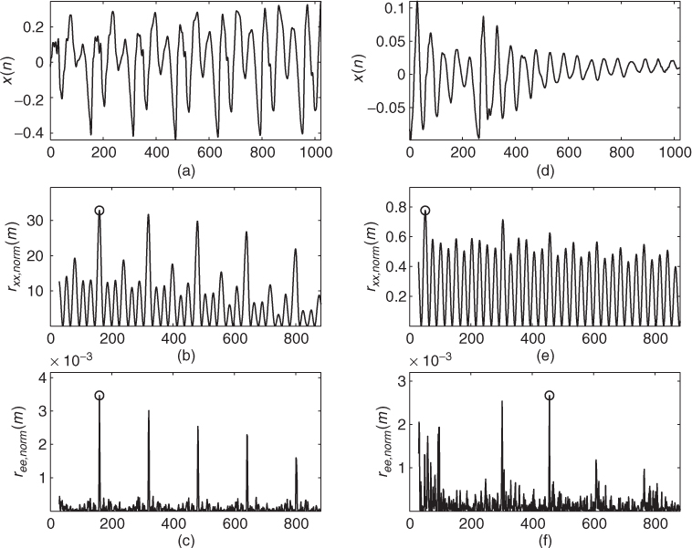
Figure 9.22 shows the detected pitch-lag candidates and the corresponding frequencies over time for a signal segment of Suzanne Vega's ‘Tom's Diner.’ It is the same example as presented in Figure 9.11 where also a spectrogram of this sound signal is given. The top plot of Figure 9.22 shows the detected pitch-lag candidates computed by the LTP algorithm applied to the input signal. The parameter b0_thres is set to 0.3, thus b0 values in the range 0.7, …, 1.3 are accepted. The corresponding pitch frequencies in the bottom plot are computed by fp = fS/M (see (9.26)).
Figure 9.22 Pitch-lag candidates and corresponding frequencies.
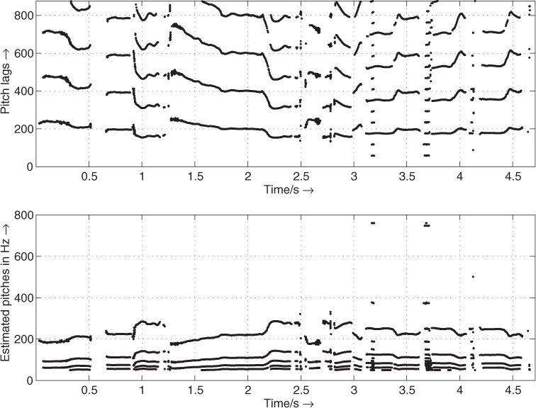
In the top plot of Figure 9.22 the lowest detected pitch lag normally corresponds to the pitch of the signal frame. The algorithm detects other candidates at multiples of this pitch lag. In some parts of this signal (for example, between 3 and 4 s) the third harmonic of the real pitch is more dominant than the fundamental frequency. In these parts the lowest detected pitch lag is not the one to be chosen. In this time-domain approach the precision of the detected pitch lags can be improved if the greatest common divisor of the pitch-lag candidates is used. The algorithm computes only integer-valued pitch-lag candidates. LTP with a higher precision (non-integer pitch lag M) is presented in [LVKL96, KA90]. As in the FFT-based approach a post-processing should be applied to choose one of the detected candidates for each frame. For a more reliable pitch estimation both time and frequency domain approaches may be combined.
The following M-file 9.12 presents an implementation of a pitch tracker based on the LTP approach.
M-file 9.12 (Pitch_Tracker_LTP.m)
% Pitch_Tracker_LTP.m [DAFXbook, 2nd ed., chapter 9]
%===== This function demonstrates a pitch tracker based
%===== on the Long-Term Prediction
%----- initializations -----
fname='Toms_diner';
n0=2000; % start index
n1=210000;
K=200; % hop size for time resolution of pitch estimation
N=1024; % block length
% checked pitch range in Hz:
fmin=50;
fmax=800;
b0_thres=.2; % threshold for LTP coeff
p_fac_thres=1.05; % threshold for voiced detection
% deviation of pitch from mean value
[xin,Fs]=wavread(fname,[n0 n0]); %get Fs
% lag range in samples:
lmin=floor(Fs/fmax);
lmax=ceil(Fs/fmin);
pre=lmax; % number of pre-samples
if n0-pre<1
n0=pre+1;
end
Nx=n1-n0+1; % signal length
blocks=floor(Nx/K);
Nx=(blocks-1)*K+N;
[X,Fs]=wavread(fname,[n0-pre n0+Nx]);
X=X(:,1)';
pitches=zeros(1,blocks);
for b=1:blocks
x=X((b-1)*K+(1:N+pre));
[M, F0]=find_pitch_ltp(x, lmin, lmax, N, Fs, b0_thres);
if ∼isempty(M)
pitches(b)=Fs/M(1); % take candidate with lowest pitch
else
pitches(b)=0;
end
end
%----- post-processing -----
L=9; % number of blocks for mean calculation
if mod(L,2)==0 % L is even
L=L+1;
end
D=(L-1)/2; % delay
h=ones(1,L)./L; % impulse response for mean calculation
% mirror start and end for “non-causal” filtering:
p=[pitches(D+1:-1:2), pitches, pitches(blocks-1:-1:blocks-D)];
y=conv(p,h); % length: blocks+2D+2D
pm=y((1:blocks)+2*D); % cut result
Fac=zeros(1,blocks);
idx=find(pm∼=0); % don't divide by zero
Fac(idx)=pitches(idx)./pm(idx);
ii=find(Fac<1 & Fac∼=0);
Fac(ii)=1./Fac(ii); % all non-zero element are now > 1
% voiced/unvoiced detection:
voiced=Fac∼=0 & Fac<p_fac_thres;
T=40; % time in ms for segment lengths
M=round(T/1000*Fs/K); % min. number of blocks in a row
[V,p2]=segmentation(voiced, M, pitches);
p2=V.*p2; % set pitches to zero for unvoiced
figure(1),clf;
time=(0:blocks-1)*K+1; % start sample of blocks
time=time/Fs; % time in seconds
t=(0:length(X)-1)/Fs; % time in sec for original
subplot(211)
plot(t, X),title('original x(n)'),
axis([0 max([t,time]) -1.1*max(abs(X)) 1.1*max(abs(X))])
subplot(212)
idx=find(p2∼=0);
plot_split(idx,time, p2),title('pitch in Hz'),
xlabel('time/s ightarrow'),
axis([0 max([t,time]) .9*min(p2(idx)) 1.1*max(p2(idx))])
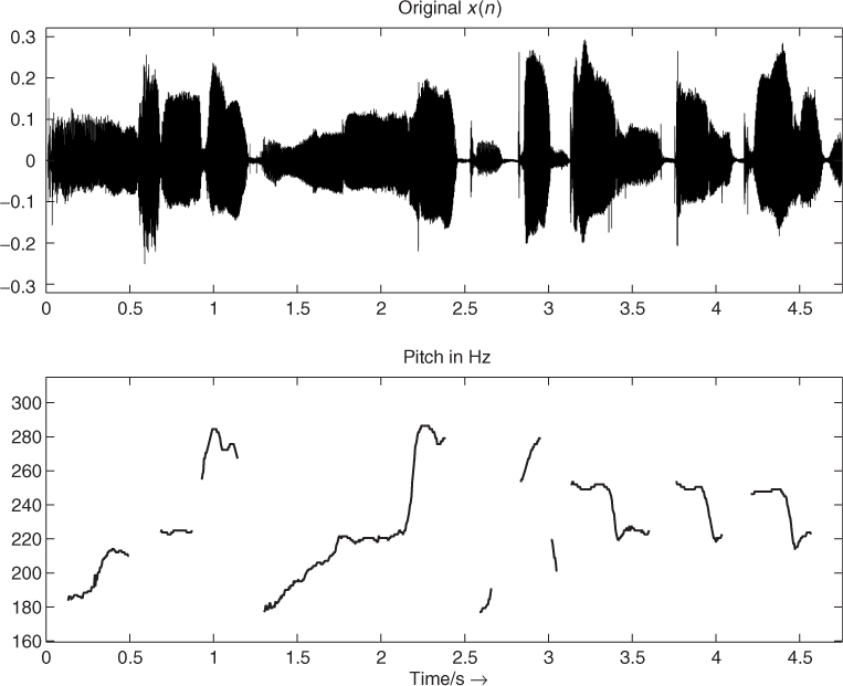
The result of the presented pitch-tracking algorithm is illustrated in Figure 9.23. The bottom plot shows the pitch over time calculated using the LTP method. In comparison to the FFT-based approach in Figure 9.12, the FFT approach performs better in the regions where unvoiced parts occur. The described approach performs well for singing-voice examples. The selection of the post-processing strategy depends on the specific sound or signal.
Figure 9.23 Pitch over time using the long-term prediction method for a signal segment of Suzanne Vega's ‘Tom's Diner.’
9.2.5 Spatial Hearing Cues
Spatial hearing relates to source localization (in terms of distance, azimuth, elevation), motion (Doppler), and directivity, as well as to the room effect (reverberation, echo). Computational models that perform auditory scene analysis (ASA) rely on both inter-aural intensity (IID) and inter-aural time (ITD) differences [Bla83] in order to estimate the source azimuth. Elevation and distance are more difficult to estimate, as they involve modeling knowing or estimating the head-related transfer function. While it is quite complex matter to properly deconvolve a signal in order to remove its reverberation, the same deconvolution techniques can perform a bit better to estimate a room echo. In any case, spatial-related sound features extracted from ASA software are good starting points for building an adaptive control that depends on spatial attributes.
9.2.6 Timbral Features
Timbre is the most complex perceptual attribute for sound analysis. Here is a reminder of some of the sound features related to timbre:
- Brightness, correlated to spectral centroid [MWdSK95]—itself related to spectral slope, zero-crossing rate, and high frequency content [MB96]—and computed with various models [Cab99].
- Quality and noisiness, correlated to signal-to-noise ratio and to voiciness.
- Texture, related to jitter and shimmer of partials/harmonics [DT96a] (resulting from a statistical analysis of the partials' frequencies and amplitudes), to the balance of odd/even harmonics (given as the peak of the normalized auto-correlation sequence situated half way between the first- and second-highest peak values [AKZ02a]) and to harmonicity.
- Formants and especially vowels for the voice [Sun87] extracted from the spectral envelope; the spectral envelope of the residual; and the mel-frequency critical bands (MFCC), perceptual correlate of the spectral envelope.
Again, specialized software for computing perceptual models of timbre parameters are also good sources of sound features. For instance, PsySound performs the computation of brightness and roughness models, among others. For implementation purposes, sound features will be described by the family of signal-processing technique/domain used to compute them.
Auto-correlation Features
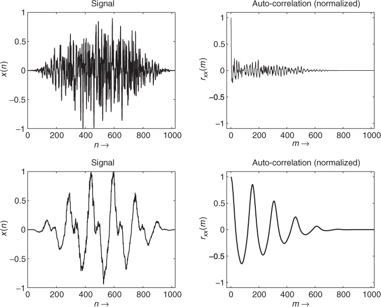
We can extract important features from the auto-correlation sequence of a windowed signal: an estimation of the harmonic/non-harmonic content of a signal, the odd/even harmonics ratio in the case of harmonic sounds, and a voiced/unvoiced part in a speech signal. Several algorithms which determine whether a speech frame is voiced or unvoiced are known from speech research [Hes83]. Voiced/unvoiced detection is used either for speech recognition or for synthesis. For digital audio effects, such a feature is useful as a control parameter for an adaptive audio effect. The first peak value of the normalized auto-correlation sequence rxx(m) for m > 0 is a good indicator of the unvoiced or voiced part of a signal, as shown in Figure 9.24. When sounds are harmonic, the first auto-correlation peak (m > 0) on the abscissa corresponds to the pitch period of this sound. The value of this peak will be maximum if the sound is harmonic and minimum if the sound is noisy. If a window is used, which gives a better estimate for pitch extraction, this peak value will not go to one, but will be weighted by the auto-correlation of the two windows. This first peak value will be denoted pv at m0 and is a good indication of voiced/noisy parts in a spoken or sung voice [BP89]. From then, voiciness is defined as the ratio between the amplitude of the first peak m > 0 divided by the auto-correlation for m = 0, which is the signal amplitude
9.41 ![]()
In the case of harmonic sounds, it can be noted that the odd/even harmonics ratio can also be retrieved from the value at half of the time lag of the first peak. The percentage of even harmonics amplitudes is given as
9.42 ![]()
Figure 9.24 Unvoiced (upper part) and voiced (lower part) signals and the corresponding auto-correlation sequence rxx(m).
An alternative computation of the auto-correlation sequence can be performed in the frequency domain [OS75]. Normally, the auto-correlation is computed from the power spectrum |X(k)|2 of the input signal by ![]() . Here, we perform the IFFT of the magnitude |X(k)| (square root of the power spectrum), which is computed from the FFT of a windowed signal. This last method is illustrated by the following M-file 9.13 that leads to a curve following the voiced/unvoiced feature, as shown in Figure 9.25.
. Here, we perform the IFFT of the magnitude |X(k)| (square root of the power spectrum), which is computed from the FFT of a windowed signal. This last method is illustrated by the following M-file 9.13 that leads to a curve following the voiced/unvoiced feature, as shown in Figure 9.25.
M-file 9.13 (UX_voiced.m)
% UX_voiced.m
% feature_voice is a measure of the maximum of the second peak
% of the acf
clear;clf
%----- USER DATA -----
[DAFx_in, FS] = wavread('x1.wav'),
hop = 256; % hop size between two FFTs
WLen = 1024; % length of the windows
w = hanningz(WLen);
%----- some initializations -----
WLen2 = WLen/2;
tx = (1:WLen2+1)';
normW = norm(w,2);
coef = (WLen/(2*pi));
pft = 1;
lf = floor((length(DAFx_in) - WLen)/hop);
feature_voiced = zeros(lf,1);
tic
%===========================================
pin = 0;
pend = length(DAFx_in) - WLen;
while pin<pend
grain = DAFx_in(pin+1:pin+WLen).* w;
f = fft(grain)/WLen2;
f2 = real(ifft(abs(f)));
f2 = f2/f2(1);
[v,i1] = min(f2(1:WLen2)>0.);
f2(1:i1) = zeros(i1,1);
[v,imax] = max(f2(1:WLen2));
feature_voiced(pft) = v;
pft = pft + 1;
pin = pin + hop;
end
% ===========================================
toc
subplot(2,1,1)
plot(feature_voiced)
Figure 9.25 Vocal signal and the ‘voiced/unvoiced’ feature pv(n).

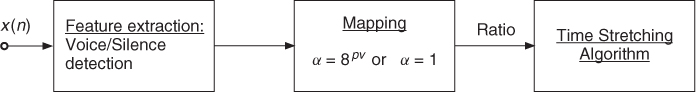
A particular way to use this feature is the construction of an adaptive time-stretching effect, where the stretching ratio α depends on this feature according to a mapping function α = 8pv (see Figure 9.26). The time-stretching ratio will vary from 1 to 8, depending on the evolution of pv over time. A threshold detector can help to force this ratio to 1 in the case of silence. This leads to great improvements over regular time-stretching algorithms.
Figure 9.26 Adaptive time stretching based on auto-correlation feature.
Center of Gravity of a Spectrum (Spectral Centroid)
An important feature of a sound is the evolution of the ‘richness of harmonics’ over time. It has been clearly pointed out at the beginning of computer music that sounds synthesized with a fixed waveform give only static sounds, and that the sound's harmonic content must evolve with time to give a lively sound impression. So algorithmic methods of synthesis have used this variation: additive synthesis uses the balance between harmonics or partials, waveshaping or FM synthesis use an index which changes the richness by the strength of the components.
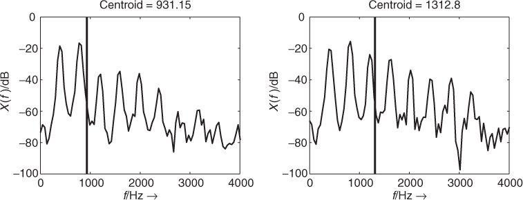
A good indication of the instantaneous richness of a sound can be measured by the center of gravity of its spectrum, as depicted in Figure 9.27. A sound with a fixed pitch, but with stronger harmonics has a higher center of gravity. It should be noted here that this center of gravity is linked to the pitch of the sound, and that this should be taken into account during the use of this feature. Thus, a good indicator of the instantaneous richness of a sound can be the ratio of the center of gravity divided by the pitch.
Figure 9.27 Center of gravity of a spectrum as a good indicator of the richness of a harmonic sound.
A straightforward method of calculating this centroid can be achieved inside an FFT/IFFT-based analysis-synthesis scheme. The spectral centroid is at the center of the spectral energy distribution and can be calculated by
The centroid is defined by the ratio of the sum of the magnitudes multiplied by the corresponding frequencies divided by the sum of the magnitudes and it is also possible to use the square of the magnitudes
9.44 
Another method working in the time domain makes use of the property of the derivative of a sinusoid which gives ![]() with
with ![]() . If we can express the input signal by a sum of sinusoids according to
. If we can express the input signal by a sum of sinusoids according to
9.45 
the derivative of the input signal leads to
9.46 
The spectral centroid can then be computed according to (9.43) by the ratio of the RMS value of the derivative of the input signal divided by the RMS value of the input signal itself. The derivative of the discrete-time input signal x(n) can be approximated by Δx(n) = x(n) − x(n − 1). The described time-domain method is quite effective because it does not need any FFT and is suitable for real-time applications. The following M-file 9.14 illustrates these possibilities.
M-file 9.14 (UX_centroid.m)
% UX_centroid.m
[DAFXbook, 2nd ed., chapter 9]
% feature_centroid1 and 2 are centroids
% calculate by two different methods
clear;clf
%----- USER DATA -----
[DAFx_in, FS] = wavread('x1.wav'),
hop = 256; % hop size between two FFTs
WLen = 1024; % length of the windows
w = hanningz(WLen);
%----- some initializations -----
WLen2 = WLen/2;
tx = (1:WLen2+1)';
normW = norm(w,2);
coef = (WLen/(2*pi));
pft = 1;
lf = floor((length(DAFx_in) - WLen)/hop);
feature_rms = zeros(lf,1);
feature_centroid = zeros(lf,1);
feature_centroid2 = zeros(lf,1);
tic
%===========================================
pin = 0;
pend = length(DAFx_in) - WLen;
while pin<pend
grain = DAFx_in(pin+1:pin+WLen).* w;
feature_rms(pft) = norm(grain,2) / normW;
f = fft(grain)/WLen2;
fx = abs(f(tx));
feature_centroid(pft) = sum(fx.*(tx-1)) / sum(fx);
fx2 = fx.*fx;
feature_centroid2(pft) = sum(fx2.*(tx-1)) / sum(fx2);
grain2 = diff(DAFx_in(pin+1:pin+WLen+1)).* w;
feature_deriv(pft) = coef * norm(grain2,2) / norm(grain,2);
pft = pft + 1;
pin = pin + hop;
end
% ===========================================
toc
subplot(4,1,1); plot(feature_rms); xlabel('RMS')
subplot(4,1,2); plot(feature_centroid); xlabel('centroid 1')
subplot(4,1,3); plot(feature_centroid2); xlabel('centroid 2')
subplot(4,1,4); plot(feature_deriv); xlabel('centroid 3')
For each method the center of gravity is calculated in frequency bins. Figure 9.28 illustrates the results for each method. It can be seen at the end of a flute sound that the centroid parameter is very important: the variations of the centroid are quite independent of the RMS values of the signal. The centroid takes some time to oscillate and then is maintained until the end of the sound. An alternative has been proposed, so that the centroid tends to 0 when the sound intensity level also tends to 0. It consists of adding a constant of small value in the centroid denominator [Bea82]:
9.47 
An artifact of this computation is that it alway biases the centroid value from the usual formulation one, whereas the following computation only biases for low signal intensity levels:
9.48 
Figure 9.28 Spectral centroid computation in frequency and time domain. Plots (b)–(d) show the centroids in bins, where the corresponding tone pitch is given by ![]() (with FFT length N and sampling frequency fS).
(with FFT length N and sampling frequency fS).
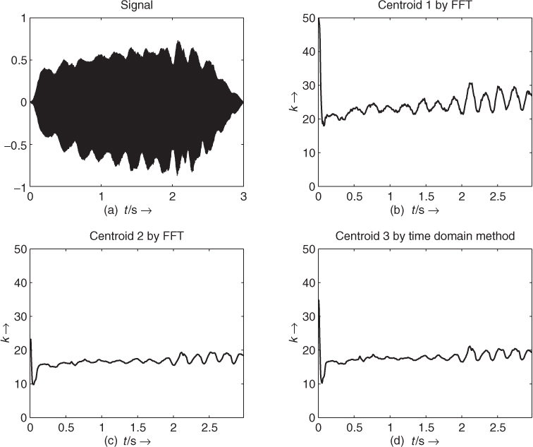
A digital effect which relies on the spectral centroid feature is the mimicking of a natural sound by a synthetic one. As an example, we can use a waveshaping synthesis method. This method calculates a synthetic sound by distorting a sine wave with the help of a waveshaping function (also called nonlinear transfer function) and multiplying the result by an amplitude variation (see Figure 9.29). The waveshaping function is usually a polynomial, because this function can be calculated with the aim of having a fixed output spectrum [Arf79, Bru79]. So apart from the pitch of the sine wave, this method relies on the evolution of two parameters: the amplitude of the sine wave, which is called the ‘index’ because the sine wave is used as an input to the waveshaping function, and an amplitude factor, which is used as an amplitude envelope. If we extract the centroid and the RMS evolution from a natural sound, as well as the pitch, we can compute an index proportional to the ratio of the centroid towards the pitch (this proportional factor, apart from a necessary normalization, drives the general brightness of the sound) and an amplitude factor proportional to the extracted RMS feature. Thus we obtain a synthetic sound that retains some characteristics of the initial sound and is given by
9.49 
The mimicking is improved when the waveshaping function is calculated for the spectrum at one point of the initial sound. Two other further improvements can be added: an amplitude normalization factor due to the fact that the index should only change the centroid and not the amplitude, and a correcting factor for the index due to the fact that the index and centroid of the synthetic sound have no reason to be in a linear relationship. But even the simple process we have described gives a variety of allotropic sounds which all resemble the original in some way, but are purely harmonic and do not contain any noisy components.
Figure 9.29 Mimicking with waveshaping.
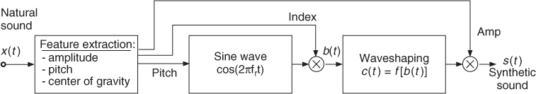
Features from Harmonic Partials
Once a spectral model of a harmonic sound is computed, various sound features can be extracted from the harmonic partial amplitude and frequency, apart from the harmonic centroid we have already presented. The relative percentage of amplitude or energy of the even and odd harmonics can be computed as
9.50 
9.51 
These features are called even/odd harmonic ratios. Such computation is more accurately than the one proposed with the auto-correlation function, because the latter computes the amplitude of even harmonics relative to the whole sound amplitude, not only that of the harmonic partials. Alternatives are the ratio of odd versus even harmonics and the ratio of even versus odd harmonics.
The tristimulus is a timbral descriptor that was derived for sounds as an equivalent of the color attributes for vision [PJ82]. It is computed by
9.52 ![]()
9.53 
9.54 
From these equations, it follows that T1(m) describes the strength of fundamental amplitude compared to all harmonics. T2(m) describes how strong are the middle frequency harmonics and T3(m) describes how strong are the higher harmonic amplitudes. As for the spectral centroid, it can be modified using energies instead of amplitudes, and truncating the denominator for low-level signals, in which case the tristimuli becomes:
9.55 
9.56 
9.57 
9.2.7 Statistical Features
As an example, Dubnov [DT96b] has obtained the classification of instrumental timbres on a 2-D map by using skew and kurtosis. These features can help in defining the texturization of a sound. The texture of a sound is very difficult to evaluate: why a trumpet does not sound like a string does not rely only on a spectral richness. The way the individual components are synchronized or not is an important key for defining a texture. Many other features can be extracted from a sound [HB98, RDS+99, DH00], just to mention a few from a very active field of research.