
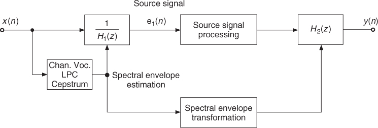
Digital audio effects based on source-filter processing extract the spectral envelope and the source (excitation) signal from an input signal, as shown in Figure 8.2. The input signal is whitened by the filter 1/H1(z), which is derived from the spectral envelope of the input signal. In signal-processing terms, the spectral envelope is given by the magnitude response |H1(f)| or its logarithm log|H1(f)| in dB. This leads to extraction of the source signal e1(n) which can be further processed, for example, by time-stretching or pitch-shifting algorithms. The processed source signal is then finally filtered by H2(z). This filter is derived from the modified spectral envelope of the input signal or another source signal.
Figure 8.2 Spectrum estimation (Channel vocoder, Linear Predictive Coding or Cepstrum) and source-signal extraction for individual processing.
8.2.1 Channel Vocoder
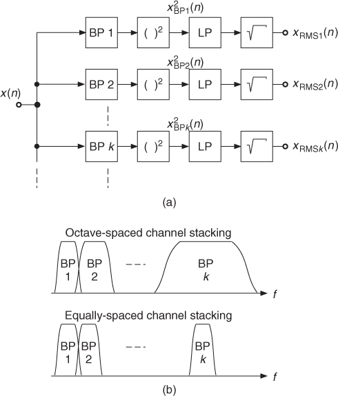
If we filter a sound with a bank of bandpass filters and calculate the RMS value for each bandpass signal, we can obtain an estimation of the spectral envelope (see Figure 8.3). The parameters of the filters for each channel will of course affect the precision of the measurement, as well as the delay between the sound input and the spectral calculation. The RMS calculation parameters are also a compromise between good definition and an acceptable delay and trail effect. The spectral estimation is valid around the center frequency of the filters. Thus the more channels there are, the more frequency points of the spectral envelope are estimated. The filter bank can be defined on a linear scale, in which case every filter of the filter bank can be equivalent in terms of bandwidth. It can also be defined on a logarithmic scale. In this case, this approach is more like an “equalizer system” and the filters, if given in the time domain, are scaled versions of a mother filter.
Figure 8.3 (a) Channel vocoder and (b) frequency stacking.
The channel-vocoder algorithm shown in Figure 8.3 works in the time domain. There is, however, a possible derivation where it is possible to calculate the spectral envelope from the FFT spectrum, thus directly from the time-frequency representations. A channel can be represented in the frequency domain, and the energy of an effective channel filter can be seen as the sum of the elementary energies of each bin weighted by this channel filter envelope. The amplitude coming out of this filter is then the square root of these energies.
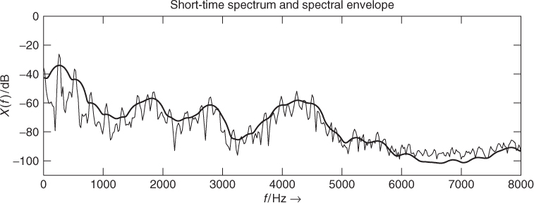
In the case of filters with equally spaced channel stacking (see Figure 8.3b), it is even possible to use a short-cut for the calculation of this spectral envelope: the spectral envelope is the square root of the filtered version of the squared amplitudes. This computation can be performed by a circular convolution ![]() in the frequency domain, where w(k) may be a Hanning window function. The circular convolution is accomplished by another FFT/IFFT filtering algorithm. The result is a spectral envelope, which is a smoothing of the FFT values. An example is shown in Figure 8.4.
in the frequency domain, where w(k) may be a Hanning window function. The circular convolution is accomplished by another FFT/IFFT filtering algorithm. The result is a spectral envelope, which is a smoothing of the FFT values. An example is shown in Figure 8.4.
Figure 8.4 Spectral envelope computation with a channel vocoder.
The following M-file 8.1 defines channels in the frequency domain and calculates the energy in dB inside successive channels of that envelope.
M-file 8.1 (UX_specenv.m)
s_win = 2048;
w = hanning(s_win, ’periodic’);
buf = y(offset:offset+s_win-1).*w;
f = fft(buf)/(s_win/2);
freq = (0:1:s_win-1)/s_win*44100;
flog = 20*log10(0.00001+abs(f));
%---- frequency window ----
nob = input(’number of bins must be even = ’);
w = hanning(nob, ’periodic’);
w1 = hanning(nob, ’periodic’);
w1 = w1./sum(w1);
f_channel = [zeros((s_win-nob)/2,1); w1; zeros((s_win-nob)/2,1)];
%---- FFT of frequency window ----
fft_channel = fft(fftshift(f_channel));
f2 = f.*conj(f); % Squared FFT values
%---- circular convolution by FFT-Multiplication-IFFT ----
energy = real(ifft(fft(f2).*fft_channel));
flog_rms = 10*log10(abs(energy)); % 10 => combination with sqrt operation
%---- plot result ----
subplot(2,1,1); plot(freq,flog,freq,flog_rms);
ylabel(’X(f)/dB’);
xlabel(’f/Hz ightarrow’); axis([0 8000 -110 0]);
title(’Short-time spectrum and spectral envelope’);
The program starts with the calculation of the FFT of a windowed frame, where w is a Hanning window in this case. The vector y contains the sound and a buffer buf contains a windowed segment. In the second part of this program fchannel represents the envelope of the channel with a FFT representation. Here it is a Hanning window of width nob, which is the number of frequency bins. The calculation of the weighted sum of the energies inside a channel is performed by a convolution calculation of the energy pattern and the channel envelope. Here, we use a circular convolution with an FFT-IFFT algorithm to easily retrieve the result for all channels. In a way it can be seen as a smoothing of the energy pattern. The only parameter is the envelope of the channel filter, hence the value of nob in this program. The fact that it is given in bins and that it should be even is only for the simplification of the code. The bandwidth is given by nob![]() (N is the length of the FFT).
(N is the length of the FFT).
8.2.2 Linear Predictive Coding (LPC)
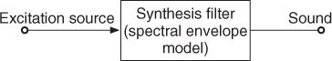
One way to estimate the spectral envelope of a sound is directly based on a simple sound-production model. In this model, the sound is produced by passing an excitation source (source signal) through a synthesis filter, as shown in Figure 8.5. The filter models the resonances and has therefore only poles. Thus, this all-pole filter represents the spectral envelope of the sound. This model works well for speech, where the synthesis filter models the human vocal tract, while the excitation source consists of pulses plus noise [Mak75]. For voiced sounds the periodicity of the pulses determines the pitch of the sound, while for unvoiced sounds the excitation is noise-like.
Figure 8.5 Sound production model: the synthesis filter represents the spectral envelope.
The retrieval of the spectral envelope from a given sound at a given time is based on the estimation of the all-pole synthesis filter mentioned previously. This approach is widely used for speech coding and is called linear predictive coding (LPC) [Mak75, MG76].
Analysis/Synthesis Structure
In LPC the current input sample x(n) is approximated by a linear combination of past samples of the input signal. The prediction of x(n) is computed using an FIR filter by
8.1 
where p is the prediction order and ak are the prediction coefficients. The difference between the original input signal x(n) and its prediction ![]() is evaluated by
is evaluated by
The difference signal e(n) is called residual or prediction error and its calculation is depicted in Figure 8.6 where the transversal (direct) FIR filter structure is used.
Figure 8.6 Transversal FIR filter structure for the prediction-error calculation.

With the z-transform of the prediction filter
8.3 
Equation (8.2) can be written in the z-domain as
8.4 ![]()
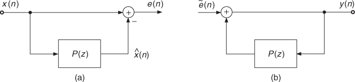
Figure 8.7a illustrates the last equation. The illustrated structure is called feed-forward prediction where the prediction is calculated in the forward direction from the input signal.
Figure 8.7 LPC structure with feed-forward prediction: (a) analysis, (b) synthesis.
Defining the prediction error filter or inverse filter
8.5 
the prediction error is obtained as
8.6 ![]()
The sound signal is recovered by using the excitation signal ![]() as input to the all-pole filter
as input to the all-pole filter
8.7 ![]()
This yields the output signal
8.8 ![]()
where H(z) can be realized with the FIR filter P(z) in a feedback loop, as shown in Figure 8.4. If the residual e(n), which is calculated in the analysis stage, is fed directly into the synthesis filter, the input signal x(n) will be ideally recovered.
The IIR filter H(z) is termed synthesis filter or LPC filter and represents the spectral model—except for a gain factor—of the input signal x(n). As mentioned previously, this filter models the time-varying vocal tract in the case of speech signals.
With optimal filter coefficients, the residual energy is minimized. This can be exploited for efficient coding of the input signal where the quantized residual ![]() is used as excitation to the LPC filter.
is used as excitation to the LPC filter.
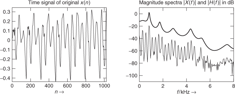
Figure 8.8 shows an example where for a short block of a speech signal an LPC filter of order p = 50 is computed. In the left plot the time signal is shown, while the right plot shows both the spectra of the input signal and of the LPC filter H(z). In this example the autocorrelation method is used to calculate the LPC coefficients. The MATLAB® code for this example is given by M-file 8.2 (the used function calc_lpc will be explained later).
M-file 8.2 (figure8_08.m)
N = 1024; % block length
Nfft = 1024; % FFT length
p = 50; % prediction order
n1 = n0+N-1; % end index
[xin,Fs] = wavread(fname,[n0 n1]);
x = xin(:,1)’; % row vecor of left channel
win = hamming(N)’; % window for input block
a = calc_lpc(x.*win,p); % calculate LPC coeffs
% a = [1, -a_1, -a_2,..., -a_p]
Omega = (0:Nfft-1)/Nfft*Fs/1000; % frequencies in kHz
offset = 20*log10(2/Nfft); % spectrum offset in dB
A = 20*log10(abs(fft(a,Nfft)));
H = -A+offset;
X = 20*log10(abs(fft(x.*win,Nfft)));
X = X+offset;
n = 0:N-1;
Figure 8.8 LPC example for the female utterance “la” with prediction order p = 50, original signal and LPC filter.
Calculation of the Filter Coefficients
To find an all-pole filter which models a considered sound well, different approaches may be taken. Some common methods compute the filter coefficients from a block of the input signal x(n). These methods are namely the autocorrelation method [Mak75, Orf90], the covariance method [Mak75, MG76], and the Burg algorithm [Mak77, Orf90]. Since both the autocorrelation method and the Burg algorithm compute the lattice coefficients, they are guaranteed to produce stable synthesis filters, while the covariance method may yield unstable filters.
Now we briefly describe the autocorrelation method, which minimizes the energy of the prediction error e(n). With the prediction error e(n) defined in (8.2), the prediction error energy is1
8.9 ![]()
Setting the partial derivatives of Ep with respect to the filter coefficients ai (i = 1, …, p) to zero leads to
8.10 ![]()
8.11 ![]()
8.12 
Equation (8.13) is a formulation of the so-called normal equations [Mak75]. The autocorrelation sequence for a block of length N is defined by
where u(n) = x(n) · w(n) is a windowed version of the considered block x(n), n = 0, …, N − 1. Normally a Hamming window is used [O'S00]. The expectation values in (8.13) can be replaced by their approximations using the autocorrelation sequence, which gives the normal equations2
8.15 
The filter coefficients ak (k = 1, …, p), which model the spectral envelope of the used segment of x(n) are obtained by solving the normal equations. An efficient solution of the normal equations is performed by the Levinson—Durbin recursion [Mak75].
As explained in [Mak75], minimizing the residual energy is equivalent to finding a best spectral fit in the frequency domain, if the gain factor is ignored. Thus the input signal x(n) is modeled by the filter
8.16 ![]()
where G denotes the gain factor. With this modified synthesis filter the original signal is modeled using a white noise excitation with unit variance. For the autocorrelation method the gain factor is defined by [Mak75]
8.17 
with the autocorrelation sequence given in (8.14). Hence the gain factor depends on the energy of the prediction error. If |Hg(ejΩ)|2 models the power spectrum |X(ejΩ)|2, the prediction-error power spectrum is a flat spectrum with |E(ejΩ)|2 = G2. The inverse filter A(z) to calculate the prediction error is therefore also called the “whitening filter” [Mak75]. The MATLAB code of the function calc_lpc for the calculation of the prediction coefficients and the gain factor using the autocorrelation method is given by M-file 8.3.
M-file 8.3 (calc_lpc.m)
% function [a,g] = calc_lpc(x,p) [DAFXbook, 2nd ed., chapter 8]
% ===== This function computes LPC coeffs via autocorrelation method
% Similar to MATLAB function “lpc”
% !!! IMPORTANT: function “lpc” does not work correctly with MATLAB 6!
% Inputs:
% x: input signal
% p: prediction order
% Outputs:
% a: LPC coefficients
% g: gain factor
% (c) 2002 Florian Keiler
function [a,g] = calc_lpc(x,p)
R = xcorr(x,p); % autocorrelation sequence R(k) with k=-p,..,p
R(1:p) = []; % delete entries for k=-p,..,-1
if norm(R)∼=0
a = levinson(R,p); % Levinson-Durbin recursion
% a = [1, -a_1, -a_2,..., -a_p]
else
a = [1, zeros(1,p)];
end
R = R(:)’; a = a(:)’; % row vectors
g = sqrt(sum(a.*R)); % gain factor
Notice that normally the MATLAB function lpc can be used, but it does not show the expected behavior for an input signal with zeros. M-file 8.3 fixes this problem and returns coefficients ak = 0 in this case.
Figure 8.9 shows the prediction error and the estimated spectral envelope for the input signal shown in Figure 8.8. It can clearly be noticed that the prediction error has strong peaks occurring with the period of the fundamental frequency of the input signal. We can make use of this property of the prediction error signal for computing the fundamental frequency. The fundamental frequency and its pitch period can deliver pitch marks for PSOLA time-stretching or pitch-shifting algorithms, or other applications. The corresponding MATLAB code is given by M-file 8.4.
M-file 8.4 (figure8_09.m)
Nfft = 1024; % FFT length
p = 50; %prediction order
n1 = n0+N-1; %end index
pre = p; %filter order= no. of samples required before n0
[xin,Fs] = wavread(fname,[n0-pre n1]);
xin = xin(:,1)’;
win = hamming(N)’;
x = xin((1:N)+pre); % block without pre-samples
[a,g] = calc_lpc(x.*win,p); % calculate LPC coeffs and gain
% a = [1, -a_1, -a_2,..., -a_p]
g_db = 20*log10(g) % gain in dB
ein = filter(a,1,xin); % pred. error
e = ein((1:N)+pre); % without pre-samples
Gp = 10*log10(sum(x.∧2)/sum(e.∧2)) % prediction gain
Omega = (0:Nfft-1)/Nfft*Fs/1000; % frequencies in kHz
offset = 20*log10(2/Nfft); % offset of spectrum in dB
A = 20*log10(abs(fft(a,Nfft)));
H_g = -A+offset+g_db; % spectral envelope
X = 20*log10(abs(fft(x.*win,Nfft)));
X = X+offset;
n = 0:N-1;
figure(1)
clf
subplot(221)
plot(n,e)
title(’time signal of pred. error e(n)’)
xlabel(’n ightarrow’)
axis([0 N-1 -inf inf])
subplot(222)
plot(Omega,X); hold on
plot(Omega,H_g,’r’,’Linewidth’,1.5); hold off
title(’magnitude spectra |X(f)| and |Gcdot H(f)| in dB’)
xlabel(’f/kHz ightarrow’)
axis([0 8 -inf inf])
Figure 8.9 LPC example for the female utterance “la” with prediction order p = 50, prediction error and spectral envelope.
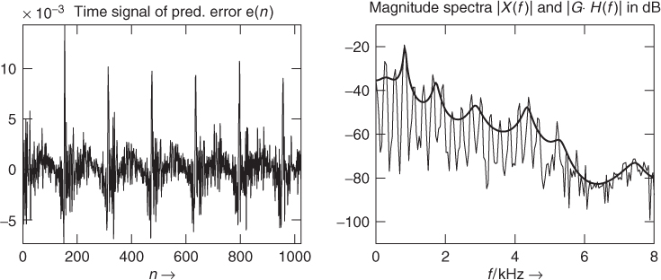
Thus for the computation of the prediction error over the complete block length, additional samples of the input signal are required. The calculated prediction error signal e(n) is equal to the source or excitation which has to be used as input to the synthesis filter H(z) to recover the original signal x(n). For this example the prediction gain, defined as
8.18 
has the value 38 dB, and the gain factor is G = − 23 dB.
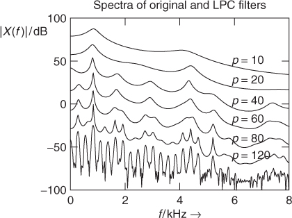
Figure 8.10 shows spectra of LPC filters at different filter orders for the same signal block as in Figure 8.8. The bottom line shows the spectrum of the signal segment where only frequencies below 8 kHz are depicted. The other spectra in this plot show the results using the autocorrelation method with different prediction orders. For clarity reasons these spectra are plotted with different offsets. It is obvious that for an increasing prediction order the spectral model gets better although the prediction gain only increases from 36.6 dB (p = 10) to 38.9 dB (p = 120).
Figure 8.10 LPC filter spectra for different prediction orders for the female utterance “la.”
In summary, the LPC method delivers a source-filter model and allows the determination of pitch marks or the fundamental frequency of the input signal.
8.2.3 Cepstrum
The cepstrum (backward spelling of “spec”) method allows the estimation of a spectral envelope starting from the FFT values X(k) of a windowed frame x(n). Zero padding and Hanning, Hamming or Gaussian windows can be used, depending on the number of points used for the spectral envelope estimation. An introduction to the basics of cepstrum-based signal processing can be found in [OS75]. The cepstrum is calculated from the discrete Fourier transform
8.19 
by taking the logarithm
and performing an IFFT of ![]() , which yields the complex cepstrum
, which yields the complex cepstrum
8.21 
The real cepstrum is derived from the real part of (8.20) given by
8.22 ![]()
and performing an IFFT of ![]() , which leads to the real cepstrum
, which leads to the real cepstrum
8.23 
Since ![]() is an even function, the inverse discrete Fourier transform of
is an even function, the inverse discrete Fourier transform of ![]() gives an even function c(n), which is related to the complex cepstrum
gives an even function c(n), which is related to the complex cepstrum ![]() by
by ![]() .
.
Figure 8.11 illustrates the computational steps for the computation of the spectral envelope from the real cepstrum. The real cepstrum c(n) is the IFFT of the logarithm of the magnitude of FFT of the windowed sequence x(n). The lowpass window for weighting the cepstrum c(n) is derived in [OS75] and is given by
8.24 
The FFT of the windowed cepstrum ![]() yields the spectral envelope
yields the spectral envelope
8.25 ![]()
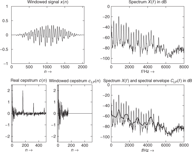
which is a smoothed version of the spectrum X(k) in dB. An illustrative example is shown in Figure 8.12. Notice that the first part of the cepstrum c(n) (0 ≤ n ≤ 150) is weighted by the “lowpass window,” yielding ![]() . The IFFT of
. The IFFT of ![]() results in the spectral envelope C(f) in dB, as shown in the lower right plot. The “highpass part” of the cepstrum c(n) (150 < n ≤ 1024) represents the source signal, where the first peak at n = 160 represents the pitch period T0 (in samples) of the fundamental frequency
results in the spectral envelope C(f) in dB, as shown in the lower right plot. The “highpass part” of the cepstrum c(n) (150 < n ≤ 1024) represents the source signal, where the first peak at n = 160 represents the pitch period T0 (in samples) of the fundamental frequency ![]() Hz. Notice also, although the third harmonic is higher than the fundamental frequency, as can be seen in the spectrum of the segment, the cepstrum method allows the estimation of the pitch period of the fundamental frequency by searching for the time index of the first highly significant peak value in the cepstrum c(n) after the “lowpass” part can be considered to have vanished. The following M-file 8.5 demonstrates briefly the way a spectral envelope can be calculated via the real cepstrum.
Hz. Notice also, although the third harmonic is higher than the fundamental frequency, as can be seen in the spectrum of the segment, the cepstrum method allows the estimation of the pitch period of the fundamental frequency by searching for the time index of the first highly significant peak value in the cepstrum c(n) after the “lowpass” part can be considered to have vanished. The following M-file 8.5 demonstrates briefly the way a spectral envelope can be calculated via the real cepstrum.
M-file 8.5 (UX_specenvceps.m)
% N1: cut quefrency
WLen = 2048;
w = hanning(WLen, ’periodic’);
buf = y(offset:offset+WLen-1).*w;
f = fft(buf)/(WLen/2);
flog = 20*log10(0.00001+abs(f));
subplot(2,1,1); plot(flog(1:WLen/2));
N1 = input(’cut value for cepstrum’);
cep = ifft(flog);
cep_cut = [cep(1); 2*cep(2:N1); cep(N1+1); zeros(WLen-N1-1,1)];
flog_cut = real(fft(cep_cut));
subplot(2,1,2); plot(flog_cut(1:WLen/2));
Figure 8.11 Spectral-envelope computation by cepstrum analysis.
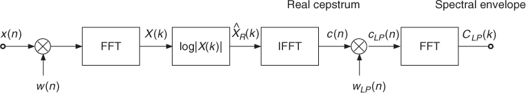
Figure 8.12 Windowed signal segment, spectrum (FFT length N = 2048), cepstrum, windowed cepstrum (N1 = 150) and spectral envelope.
In this program cep represents the cepstrum (hence the IFFT of the log magnitude of the FFT). The vector cep_cut is the version of the cepstrum with all values over the cut index set to zero. Here, we use a programming short-cut: we also remove the negative time values (hence the second part of the FFT) and use only the real part of the inverse FFT. The time indices n of the cepstrum c(n) are also denoted as “quefrencies.” The vector flog_cut is a smoothed version of flog and represents the spectral envelope derived by the cepstrum method. The only input value for the spectral envelope computation is the cut variable. This variable cut is homogeneous to a time in samples, and should be less than the period of the analyzed sound.
Source-filter Separation
The cepstrum method allows the separation of a signal y(n) = x(n) * h(n), which is based on a source and filter model, into its source signal x(n) and its impulse response h(n). The discrete-time Fourier transform ![]() is the product of two spectra: one representing the filter frequency response
is the product of two spectra: one representing the filter frequency response ![]() and the other one the source spectrum
and the other one the source spectrum ![]() . Decomposing the complex values in terms of the magnitude and phase representation, one can make the strong assumption that the filter frequency response will be real-valued and the phase will be assigned to the source signal.
. Decomposing the complex values in terms of the magnitude and phase representation, one can make the strong assumption that the filter frequency response will be real-valued and the phase will be assigned to the source signal.
The key point here is to use the mathematical property of the logarithm log(a · b) = log(a) + log(b). The real cepstrum method will perform a spectral-envelope estimation based on the magnitude according to
![]()
In musical terms separating ![]() from
from ![]() is to keep the slow variation of
is to keep the slow variation of ![]() as a filter and the rapid ones as a source. In terms of signal processing we would like to separate the low frequencies of the signal
as a filter and the rapid ones as a source. In terms of signal processing we would like to separate the low frequencies of the signal ![]() from the high frequencies (see Figure 8.13).
from the high frequencies (see Figure 8.13).
Figure 8.13 Separating source and filter.
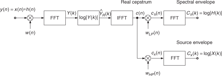
The separation of source and filter can be achieved by weighting the cepstrum c(n) = cx(n) + ch(n) with two window functions, namely the “lowpass window” ![]() and the complementary “highpass window”
and the complementary “highpass window” ![]() . This weighting yields
. This weighting yields ![]() and
and ![]() . The low time values (low “quefrencies”) for lowpass filtering
. The low time values (low “quefrencies”) for lowpass filtering ![]() give
give ![]() (spectral envelope in dB) and the high time values (higher “quefrencies”) for highpass filtering yield
(spectral envelope in dB) and the high time values (higher “quefrencies”) for highpass filtering yield ![]() (source estimation). The calculation of
(source estimation). The calculation of ![]() gives the magnitude response
gives the magnitude response ![]() . From this magnitude transfer function we can compute a zero-phase filter impulse response according to
. From this magnitude transfer function we can compute a zero-phase filter impulse response according to
8.26 ![]()
The cepstrum method has a very good by-product. The combination of the highpass filtered version of the cepstrum and the initial phases from the FFT gives a spectrum that can be considered as the source spectrum in a source-filter model. This helps in designing audio effects based on such a source-filter model. The source signal x(n) can be derived from the calculation of exp(Cx(k)) = |X(k)| and the initial phase taken from ![]() by performing the IFFT of
by performing the IFFT of ![]() according to
according to
8.27 ![]()
For finding a good threshold between low and high quefrencies, one can make use of the fact that quefrencies are time variables, and whenever the sound is periodic, the cepstrum shows a periodicity corresponding to the pitch. Hence this value is the upper quefrency or upper time limit for the spectral envelope. A low value will smoothen the spectral envelope, while a higher value will include some of the harmonic or partial peaks in the spectral envelope.
Hints and Drawbacks
- “Lowpass filtering” is performed by windowing (zeroing values over a “cut quefrency”). This operation corresponds to filtering in the frequency domain with a
 behavior. An alternative version is to use a smooth transition instead of an abrupt cut in the cepstrum domain.
 - The cepstrum method will give a spectral estimation that smoothes the instantaneous spectrum. However, log values can go to −∞ for a zero value in the FFT. Though this rarely happens with sounds coming from the real world, where the noise level prevents such values, a good prevention is the limitation of the log value. In our implementation the addition of a small value 0.00001 to the FFT values limits the lower log limit to −100 dB. Once again, an alternative to this bias applied to all values consists in truncating instead. Then, the following line from MATLAB code 8.5
flog=20*log10(0.00001+abs(f));
becomes
flog=20*log10(max(0.00001,abs(f)));
The artifact is not the same, as the spectrum shape is no more shifted, but clipped when below the threshold value.
- Though the real cepstrum is widely used, it is also possible to use the complex cepstrum to perform an estimation of the spectral envelope. In this case the spectral envelope will be defined by a complex FFT.
The spectral envelope estimation with the cepstrum has at least the three following limitations:
- The spectral envelope does not exactly link the spectral peaks (approximation): the spectral envelope estimated being a smoothing of the spectrum, nothing implies that the spectral envelope obtained should have the exact same values as the frequency peaks when it crosses them. And in fact, this does not happen.
- The spectral envelope has a behavior which depends on the choice of the cut-off quefrency (and number of cepstral coefficients): for too small values of the cut-off quefrency, the envelope becomes too smooth, whereas for too high values, the envelope follows the spectrum too much, showing anti-resonances between spectral peaks. Another situation where the cepstrum is not efficient is for high-pitched sounds: the number of spectral peaks is too small for the algorithm to perform well, and the resulting envelope may show erratic oscillations. In fact, the cut-off quefrency should be related to the signal's fundamental frequency, which is not necessarily known at that point in the algorithm.
- The spectral envelope is poorly estimated for high-pitched sounds, since the number of partials is small and widely spaced and the algorithm performs smoothing.
For those reasons, alternatives are needed to enhance the computation of spectral envelopes with the cepstrum, such as the iterative cepstrum and the discrete cepstrum. These two alternative techniques also provide cepstral coefficients that can then be used in the same way as the traditional cepstrum in order to perform source-filter separation and transformation.
Iterative Cepstrum
In order to enhance the computation of the spectral envelope, it is possible to use an iterative algorithm which calculates only the positive difference between the instantaneous spectrum and the estimated spectral envelope in each step. The principle is explained by Laroche in [Lar95, Lar98]: We first compute Em(n, k) the initial spectral envelope of X(n, k) by the standard cepstrum technique (step m = 0). Then, we apply an iterative procedure, which for step m does the following:
1. Compute the positive difference between spectrum and spectral envelope Xm(n, k) = max(0, X(n, k) − Em(n, k))
2. Compute the spectral envelope Em+1(n, k) by cepstrum using the Xm(n, k) spectrum
3. Stop when |Xm(n, k) − Em+1(n, k)| < Δ (with Δ a given threshold).
The spectral envelope is finally given by Em+1(n, k).
While other refinements of the real cepstrum technique for estimating the spectral envelope (such as the discrete cepstrum) require the sound to be harmonic, the iterative cepstrum is similar to the real cepstrum technique: it works for any type of sound. Second, it improves it by providing a smooth envelope that goes through spectral peaks, provided that the threshold Δ is small and the maximum number of iterations is high. Because of the iterative procedure, the computation complexity is much higher, and increases exponentially as Δ decreases. The following MATLAB code 8.6 implements this iterative technique.
M-file 8.6 (UX_iterative_cepstrum.m)
% function [env,source] = iterative_cepstrum(FT,NF,order,eps,niter,Delta)
% [DAFXbook, 2nd ed., chapter 8]
% ==== This function computes the spectral enveloppe using the iterative
% cepstrum method
% Inputs:
% - FT [NF*1 | complex] Fourier transform X(NF,k)
% - NF [1*1 | int] number of frequency bins
% - order [1*1 | float] cepstrum truncation order
% - eps [1*1 | float] bias
% - niter [1*1 | int] maximum number of iterations
% - Delta [1*1 | float] spectral envelope difference threshold
% Outputs:
% - env [NFx1 | float] magnitude of spectral enveloppe
% - source [NFx1 | complex] complex source
function [env,source] = iterative_cepstrum(FT,NF,order,eps,niter,Delta)
%---- use data ----
fig_plot = 0;
%---- drawing ----
if(fig_plot), SR = 44100; freq = (0:NF-1)/NF*SR; figure(3); clf; end
%---- initializing ----
Ep = FT;
%---- computing iterative cepstrum ----
for k=1:niter
flog = log(max(eps,abs(Ep)));
cep = ifft(flog); % computes the cepstrum
cep_cut = [cep(1)/2; cep(2:order); zeros(NF-order,1)];
flog_cut = 2*real(fft(cep_cut));
env = exp(flog_cut); % extracts the spectral shape
Ep = max(env, Ep); % get new spectrum for next iteration
%---- drawing ----
if(fig_plot)
figure(3); % clf %uncomment to not superimpose curves
subplot(2,1,1); hold on
plot(freq, 20*log10(abs(FT)), ’k’)
h = plot(freq, 20*log10(abs(env)), ’k’);
set(h, ’Linewidth’, 1, ’Color’, 0.5*[1 1 1])
xlabel(’f / Hz ightarrow’); ylabel(’ ho(f) / d ightarrow’)
title(’Original spectrum and its enveloppe’)
axis tight; ax = axis; axis([0 SR/5 ax(3:4)])
drawnow
end
%---- convergence criterion ----
if(max(abs(Ep)) <= Delta), break; end
end
%---- computing source from enveloppe ----
source = FT ./ env;
Discrete Cepstrum
The discrete-cepstrum technique by Galas and Rodet [GR90] can only be used for harmonic sounds. It requires a peak-picking algorithm first (best suited after additive analysis, see Spectral Processing Chapter 10), from which it computes an exact spectral envelope which links the maximum peaks. From the spectrum X(n, k) of the current frame L amplitudes a(n, l) and corresponding frequencies f(n, l) at the peaks in the spectrum are estimated. The cepstral coefficients are then derived so that the frequency response ![]() (f) fits those {a(n, l), f(n, l)} values for l = 1, …, L. From a cepstral viewpoint, we look for the coefficients c(n), n = 0, ..., N of a real cepstrum, which corresponding frequency response
(f) fits those {a(n, l), f(n, l)} values for l = 1, …, L. From a cepstral viewpoint, we look for the coefficients c(n), n = 0, ..., N of a real cepstrum, which corresponding frequency response ![]() (f) minimizes the criterion
(f) minimizes the criterion
with w(l), l = 1, ⋯, L a series of weights related to each partial harmonic. Note that a logarithmic scale is used (it can either be 20log10, log10 or log) to ensure the constraint is related to the magnitude spectrum in dB.
Since the values of ![]() (fl) are from a symmetric spectrum (real signal), its Fourier transform can be reduced to a zero-phase cosine sum given by
(fl) are from a symmetric spectrum (real signal), its Fourier transform can be reduced to a zero-phase cosine sum given by
8.29 
The quantity ![]() we need to minimize can then be reformulated in matrix form according to
we need to minimize can then be reformulated in matrix form according to
8.30 ![]()
with the following notations:
8.31 
8.32 
8.33 
8.34 
The cepstral coefficient vector c can be estimated by
8.35 ![]()
The following MATLAB code 8.7 implements the discrete cepstrum computation.
M-file 8.7 (UX_discrete_cepstrum_basic.m)
% function cep = discrete_cepstrum_basic(F, A, order)
% [DAFXbook, 2nd ed., chapter 8]
% ==== This function computes the discrete spectrum regardless of
% matrix conditionning and singularity.
% Inputs:
% - A [1*L | float] harmonic partial amplitudes
% - F [1*L | float] harmonic partial frequencies
% - order [1*1 | int] number of cepstral coefficients
% Outputs:
% - cep [1xorder | float] cepstral coefficients
function cep = discrete_cepstrum_basic(F, A, order)
%---- initialize matrices and vectors
L = length(A);
M = zeros(L,order+1);
M = zeros(L,L);
R = zeros(order+1,1);
W = zeros(L,L);
for i=1:L
M(i,1) = 0.5;
for k=2:order+1
M(i,k) = cos(2*pi*(k-1)*F(i));
end
W(i,i) = 1; % weights = 1 by default
end
M = 2.*M;
%---- compute the solution, regardless of matric conditioning
Mt = transpose(M);
MtWMR = Mt * W * M;
cep = inv(MtWMR) * Mt * W * log(A);
Generally, the MTWM matrix is poorly conditioned or even singular, when there are a smaller number of constraints than parameters L. Since L corresponds to the number of harmonic peaks in the spectrum, it can be quite small for high-pitched sounds, resulting in such problems. Two improvements will be introduced.
Regularized Discrete Cepstrum
The criterion error ![]() , as given in (8.28), may be replaced by a composite that balances between the constraint equation
, as given in (8.28), may be replaced by a composite that balances between the constraint equation ![]() (n) and a regularization criterion, which computes the energy of the spectral envelope derivative [CLM95]. This regularization criterion is expressed as
(n) and a regularization criterion, which computes the energy of the spectral envelope derivative [CLM95]. This regularization criterion is expressed as ![]() . The new criterion is then given as
. The new criterion is then given as
8.36 
(NB: in [CLM95], there is no (1 − λ) coefficient for the first term.) From there, it is then easy to show that
8.37 
with R the diagonal matrix which elements are 8π2[0, 1, 22, 33, ..., L2]. From this, we can derive the solution given by
8.38 ![]()
This formulation only differs from [CLM95] by the ratio ![]() , because we prefer to use a value of λ ∈ [0, 1[. The corresponding M-file 8.8 shows the implementation.
, because we prefer to use a value of λ ∈ [0, 1[. The corresponding M-file 8.8 shows the implementation.
M-file 8.8 (UX_discrete_cepstrum_reg.m)
% function cep = discrete_cepstrum_reg(F, A, order, lambda)
% [DAFXbook, 2nd ed., chapter 8]
% ==== This function computes the discrete spectrum using a
% regularization function
% Inputs:
% - A [1*L | float] harmonic partial amplitudes
% - F [1*L | float] harmonic partial frequencies
% - order [1*1 | int] number of cepstral coefficients
% - lambda [1*2 | float] weighting of the perturbation, in [0,1[
% Output:
% - cep [1*order | float] cepstral coefficients
function cep = discrete_cepstrum_reg(F, A, order, lambda)
%---- reject incorrect lambda values
if lambda>=1 | lambda <0
disp(’Error: lambda must be in [0,1[’)
cep = [];
return;
end
%---- initialize matrices and vectors
L = length(A);
M = zeros(L,order+1);
R = zeros(order+1,1);
for i=1:L
M(i,1) = 1;
for k=2:order+1
M(i,k) = 2 * cos(2*pi*(k-1)*F(i));
end
end
%---- initialize the R vector values
coef = 8*(pi∧2);
for k=1:order+1
R(k,1) = coef * (k-1)∧2;
end
%---- compute the solution
Mt = transpose(M);
MtMR = Mt*M + (lambda/(1.-lambda))*diag(R);
cep = inv(MtMR) * Mt*log(A);
Less Strict and Jittered Envelope
A second improvement to relax the constraint consists in adding a number of random points around the peaks, and increasing the smoothing criterion. Then, the spectral envelope is more attracted to the region of the spectral peaks, but does not have to go through them exactly. The following MATLAB code 8.9 implements this random discrete cepstrum computation.
M-file 8.9 (UX_discrete_cepstrum_random.m)
% function cep = discrete_cepstrum_random(F, A, order, lambda, Nrand, dev)
% [DAFXbook, 2nd ed., chapter 8]
% ==== This function computes the discrete spectrum using multiples of each
% peak to which a small random amount is added, for better smoothing.
% Inputs:
% - A [1*L | float] harmonic partial amplitudes
% - F [1*L | float] harmonic partial frequencies
% - order [1*1 | int] number of cepstral coefficients
% - lambda [1v2 | float] weighting of the perturbation, in [0,1[
% - Nrand [1*1 | int] nb of random points generated per (Ai,Fi) pair
% - dev 1*2 | float] deviation of random points, with Gaussian
% Outputs:
% - cep [1*order |![]() float] cepstral coefficients
float] cepstral coefficients
function cep = discrete_cepstrum_random(F, A, order, lambda, Nrand, dev)
if lambda>=1 | lambda <0 % reject incorrect lambda values
disp(’Error: lambda must be in [0,1[’)
cep = [];
return;
end
%---- generate random points ----
L = length(A);
new_A = zeros(L*Nrand,1);
new_F = zeros(L*Nrand,1);
for k=1:L
sigA = dev * A(k);
sigF = dev * F(k);
for l=1:L
new_A((l-1)*Nrand+1) = A(l);
new_F((l-1)*Nrand+1) = F(l);
for n=1:Nrand
new_A((l-1)*Nrand+n+1) = random(’norm’, A(l), sigA);
new_F((l-1)*Nrand+n+1) = random(’norm’, F(l), sigF);
end
end
end
%---- initialize matrices and vectors
L = length(new_A);
M = zeros(L,order+1);
R = zeros(order+1,1);
for i=1:L
M(i,1) = 1;
for k=2:order+1
M(i,k) = 2 * cos(2*pi*(k-1)*new_F(i));
end
end
%---- initialize the R vector values
coef = 8*(pi∧2);
for k=1:order+1,
R(k,1) = coef * (k-1)∧2;
end
%---- compute the solution
Mt = transpose(M);
MtMR = Mt*M + (lambda/(1.-lambda))*diag(R);
cep = inv(MtMR) * Mt*log(new_A);
In conclusion, the cepstrum method allows both the separation of the audio signal into a source signal and a filter (spectral envelope) and, as a by-product, the estimation of the fundamental frequency, which has been published in [Nol64] and later reported in [Sch99]. Various refinements exist, such as the iterative cepstrum and the discrete cepstrum with an increasing computational complexity.