13.4 AM-DAFX Implementations

In this section we will describe the major steps needed to implement five different AM-DAFX. The resulting audio signal processing is the direct result of the analysis of the inter-relationship between input sources. The systems described are intended to be used for real-time signal processing. They can be implemented individually or cascaded together in order to implement an automatic audio mixer suitable for live audio mixing of music.

13.4.1 Source Enhancer

In audio mixing a common process is to enhance a source by making it more prominent. A way to achieve enhancement is by incrementing the gain of a source xμ(n) with respect of the other input sources. Performing such an action could introduce acoustic feedback or distortion if the gain needed is too large. For this reason the preferred action is to lower the gain of all sources, except for the one in need of enhancement. Although performing such an action will result in a stable enhancement of the desired source, it is not an optimal solution. This is because the sources that are not spectrally related to xμ(n) are also attenuated. In other words, if we aim to enhance a piccolo flute there should be no need to decrease a bass guitar because its spectral content shares little or no relationship with the piccolo. This type of complex frequency-dependent enhancement is familiar to audio engineers and it is what we aim to reproduce.

With this in mind we can design an AM-DAFX source enhancer whose aim is to unmask a source by applying an attenuation to the rest of the sources, relative to their spectral content. Such an enhancer should comply with the following properties:

The signal-processing section of such a device is an attenuation multiplier per input channel, and is given by ym(n) = cvm(n) · xm(n). Where the output ym(n) is the result of multipling the input signal xm(n) by the scaling factor cvm(n). Many other types of enhancements can be achieved by creative modifications of this architecture. For example, the same architecture presented here as a gain enhancer can be used to enhance signals by altering the amount of reverberation added to each channel in proportion to its spectral content. More on such an implementation and detailed references can be found in [PGR08c]. The side-chain processing architecture of such an enhancer will be detailed next.

Feature Extraction Implementation

The feature extraction algorithm we aim to design takes a digital audio input, xm(n), and outputs a data signal, fvm(n), representative of the spectral content of the input source. In order to ensure a clean acquisition we must use a data-validating algorithm. In this particular implementation we make use of an adaptive-gate algorithm. Therefore we will need the aid of an external input, xe(n), in order to derive the adaptive-gate threshold. This external input is usually taken from a measurement microphone placed in an area that is representative of the ambient noise. Such a feature extraction system is represented by fvm(n) = f(xm(n), xe(n)). Given that fvm(n) must provide us an indication of the spectral content of xm(n), a system based on spectral decomposition is appropriate, Figure 13.6.

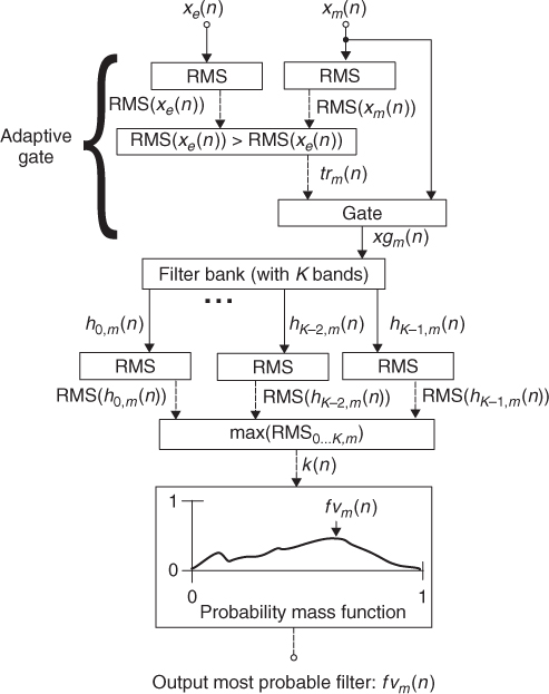
Therefore we can decompose the input xm(n) after it has been processed by the adaptive gate, xgm(n) and process it using a filter bank. The filter bank is comprised of K filters with a transfer function hk(n), where k has a valid range from 0, …, K − 1. In order to give equal opportunity for input sources to be classified as unique the filter bank can be designed to have K = M, where M corresponds to the maximum number of sources involved in the AM-DAFX and has a valid range from 0, …, M − 1. This also avoids having many sources clustered in the same spectral area. Once xgm(n) is decomposed into spectral bands we calculate the root mean square (RMS) of each k band, RMS(hk, m). Then we identify the RMS element that has the maximum RMS magnitude, max(RMS(h0…k, m)), and we store it in order to derive the probability mass function. We produce a histogram using the probability mass function k = max(RMS(h0…k, m(n))). The x axis of the histogram represents frequency bins, from 0, …, K − 1, and the y axis corresponds to the probability of the signal xm(n), to be characterised as having spectral content dominated by a given frequency bin. Given that we are calculating a probability function we must normalise all elements inside the probability mass function so that the overall addition of probabilities per bin is equal to one. This is achieved by continuously dividing the number of occurrences per bin by the total number of elements received. Finally, the maximum peak of the probability mass function must be found. This peak corresponds to the most probable spectral decomposition band fvm(n) that characterises the xm(n) under study. Under the feature extraction schema stated, fvm(n) corresponds to the most probable filter identification value and has a valid range from 0, …, K − 1. Such a feature extraction process must be implemented for all M sources.

Cross-adaptive Feature Processing

Now that we have extracted a feature that represents the spectral content of the input signal xm(n), a function that maps the inter-relationship between the spectral content of the sources must be found. Given a source to be enhanced, xμ(n), we must find a continuous function whose minima are located at fvμ(n) = k. This function should increase for filter values away from fvμ(n). The final implementation should make use of the following parameters:

• User parameters
  • μ: This is the main parameter that states which of the sources is the one to be enhanced.
  • G: Is the maximum attenuation. Any source that shares the same spectral classification as xμ(n) will have an attenuation equal to G.
  • Q: Is the amount of interaction the enhancement has with non-spectrally related sources.
• Non-user parameters
  • M: This corresponds to the total number of sources involved in cross-adaptive processing.
  • m: This tells the algorithm which source is being processed, thus getting the proper attenuation level which corresponds to a given source.

An ideal candidate to map the spectral inter-relation between channels is an inverted Gaussian. Such a function is a continuous smooth function and its minima can be made to be located at fvμ(n). Therefore we can derive

13.1

where fgm(n) is a Gaussian function, frm(n) is the frequency bin and μ(n) is the position on the frequency axis where the maximum inflection of the Gaussian function is located. In order achieve maximum attenuation at fvμ(n) we normalise and invert Equation 13.1. The user controllable G will also be included as a multiplier, so that it scales the inverted Gaussian mapping function. am(n) is the inter-source-dependent mapping function given by

13.2

For each source xm(n) we must find the assigned attenuation value am(n). Since K = M we must normalise fvm(n) with respect to M in order to obtain the correct value for frm(n). Such normalisation is given by

13.3

We require that the minima of the mapping function must be centred at fvμ(n) = k, and the algorithm has K filters with M channels. So we must normalise fvμ(n)) with respect to M,

13.4

Recall that our objective is to enhance xμ(n) with respect to the rest of sources. So we must maintain the gain of xμ(n) unchanged. This is expressed by

13.5

The cross-adaptive implementation of such an AM-DAFX is depicted in Figure 13.7. Since our approach only applies gain attenuations, it introduces no phase distortion.

The final mixture is now

13.6

where mix(n) is the overall mix after applying the cross-adaptive processing. The control attenuation for source m is given by cvm(n), where cvm(n) = 1 for m = μ. The attenuation control parameter cvm(n) varies with respect to its spectral content relationship Q, with a maximum attenuation equal to G for all sources in the same spectral category as xμ(n).

13.4.2 Panner

Stereo panning aims to transform a set of monaural signals into a two-channel signal in a pseudo-stereo field. Many methods and panning laws have been proposed, one of the most common being the sine cosine panning law. In stereo panning the ratio at which the source power has been spread between the left and the right channels determines its position. The AM-DAFX panner aims to create a satisfactory stereo mix from multi-channel audio. The proposed implementation does not take into account knowledge of physical source locations or make use of any type of contextual or visual aids. The implementation down-mixes M input sources and converts them into a two-channel mix, yL(n) and yR(n). The algorithm attempts to minimise spectral masking by allocating related source spectra to different panning space positions. The AM-DAFX also makes used of constrained rules, psychoacoustic principles and priority criteria to determine the panning positions. For this panning implementation the source inputs xm(n) have a valid range from 0, …, M − 1 and the filter bank has a total of K filters 0, …, K − 1. In order to achieve this we can apply the following panning rules:

Further information can be found in [PGR07, PGR10]. The feature extraction of the proposed AM-DAFX panner is based on accumulative spectral decomposition, in a similar way to the automatic enhancer shown in Figure 13.6. Therefore we can proceed directly to a description of the cross-adaptive feature processing of the AM-DAFX panner.

Cross-adaptive Feature Processing

Given that we have classified all xm(n) inputs according to their spectral content, a set of cross-adaptive processing functions may be established in order to determine the relationships between the spectral content of each source and its panning position. Since the algorithm aims to improve intelligibility by separating sources that have similar spectral content, while maintaining stereo balance, we must design an algorithm that makes use of the following parameters:

• User parameters
  • Um: The user priority ordering of the sources established by the user, that determines which source has more subjective importance.
  • W: The panning width scales the separation between panned sources in order to set the maximum width of the panning space.
• Non-user parameters
  • k: The filter category is used to determine if the spectral content of a source has enough high-frequency content in order for it to be panned
  • Rm: The total repetitions per classification is the number of sources in the same feature category.

In order to assign a panning position per source we must be able to identify the total number of sources in the same feature category as xm(n), denoted as Rm(n), and the relationship between the user priority, Um(n), and its spectral classification fvm(n), denoted as Pm(n). We can then calculate the panning position of a source based on the obtained parameters Rm(n) and Pm(n).

Equation 13.7 is used to obtain the total number of classification repetitions, Rm, due to other signals having the same k classification, given the initial condition R0 = 0.

13.7

Now we proceed to calculate the relationship between the user-assigned priority of a source Um(n) and its spectral classification fvm(n), we will refer to this relationship as Pm. The user-assigned priority Um has a unique value from 0, …, M − 1, the smaller the magnitude of Um, the higher the priority. The assigned priority due to being a member of the same spectral classification, Pm, has a valid range from 1 to its corresponding Rm. The lower the value taken by Pm the lower the probability of the source of being widely panned. Pm is calculated by

13.8

where the modulus of the intersection of the two sets, {Ui:fvi(n) = fvm(n)} and {Ui:Ui ≤ Um} gives us the rank position, which corresponds to the value taken by Pm.

Given Rm and Pm, we can relate them in order to obtain the panning control parameter with

13.9

and by evaluating Rm and Pm the assigned panning position can be derived. The panning position cvm(n) has a valid control range from 0 to 1, where 0 means fully panned left, 0.5 means centred and 1 means panned fully right. The panning width limit, W, can go from wide panning W = 0 to mono W = 0.5.

Finally, based on the principle that we should not pan a source if its spectral category is too low, we set cvm(n) to be centred if the spectral category of the input source fvm(n) is less than a psychoacoustically established threshold trps, (set to 200 Hz in [PGR07, PGR10]). This can be implemented by using

13.10

Given that we intend to mix all input sources by combining them in their respective stereo summing buss, the final mixture is given by

13.11

13.12

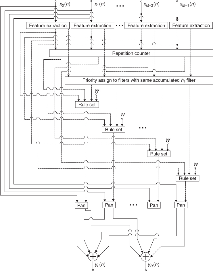
Where yL(n) and yR(n) correspond to the automatically panned stereo output of the mixing device, cvm(n) is the panning factor and xm(n) represents the input signals. Such an AM-DAFX panner implementation has been depicted in Figure 13.8.

13.4.3 Faders

In order to achieve a balanced audio mixture, careful scaling of the input signals must be achieved. The most common interface for achieving such a scaling is sliding potentiometers, commonly known as faders. Automatic fader mixers are probably the oldest form of automatic mixing, although most designs are only suitable for speech applications and are not intended for musical use. In [Dug75, Dug89] a dynamic automatic mixing implementation for music is presented. This implementation uses RMS measurements for determining the relationship between levels in order to decide the balance between microphones. One of the problems with automatic mixing implementations that use only low-level features, is that they do not take into account any perceptual attributes of the signal. Therefore a balanced RMS mixture might not be perceptually balanced. In the implementation presented here we aim to obtain a perceptual balance of all input signals. We assume that a mixture in which per-channel loudness tends to the overall average loudness is a well-balanced mixture with optimal inter-channel intelligibility.

We will use accumulative loudness measures in order to determine the perceptual level of the input signals. The main idea behind the proposed implementation is to give each channel the same probability of being heard. That is, every signal must have the same chance of masking each other. The AM-DAFX fader implementation must adapt its gain according to the loudness relationship of the individual input signals and the overall average loudness of the mix. The end result should be to scale all input signals such that they all have equal perceptual loudness. In order to achieve this we apply the following criteria:

The signal-processing section of such a device is an attenuation multiplier per input channel, and is given by ym(n) = cvm(n) · xm(n), where the output ym(n) is the result of multiplying the input signal xm(n) by the scaling factor cvm(n). Further information can be found in [PGR09a]. The side-chain architecture of such perceptually driven automatic faders will be presented next.

Feature Extraction Implementation

Our feature extraction block will make use of adaptive gating in order to avoid unwanted noise in the measured signals. The feature extraction method requires the input signals xm(n), together with an external input xe(n) in order to derive the adaptive gating function. Such a feature extraction method has a function prototype given by fvm(n) = f(xm(n), xe(n)).

Loudness is a perceptual attribute of sound. Therefore in order to be able to measure it we require a psychoacoustic model. The model proposed consists of perceptually weighting the input signal xn(n). Using a set of bi-quadratic filters whose coefficients are calculated so that the transfer function of the filters approximates loudness curves. Given that loudness curves change depending on the sound pressure level, a set of filter coefficients corresponding to different sound pressure levels can be calculated. All calculated coefficients are then stored in a look-up table. A measurement microphone xe(n), the same used for the adaptive gating, can be used to calculate the sound pressure SP(n) and retrieve the correct set of filter coefficients from the look-up table. With the aim of obtaining a clean measurement, adaptive gating can be implemented. The loudness perceptual weighting of an input signal xlm(n) is given by

13.13

where S is an averaging constant that can be used to derive longer-term loudness measurements, as opposed to instantaneous loudness, SP(n) is the sound pressure level derived from the external input and w(SP(n)) is the weighting filter loudness curves convolved with the gated input xgm(n).

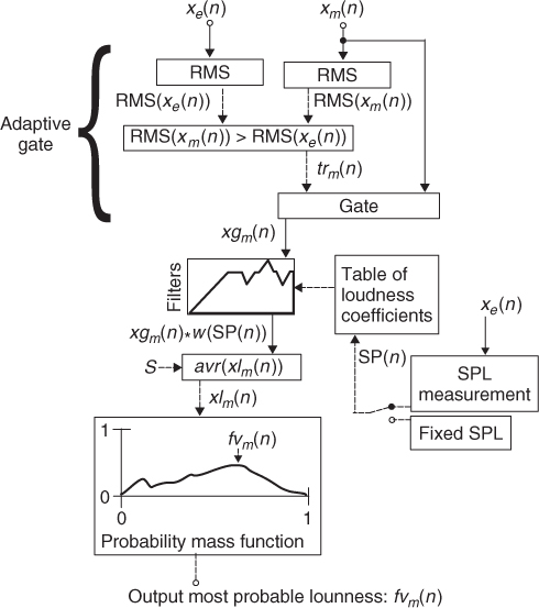
Once we have a perceptual representation of the input given by xlm(n) we can proceed to accumulate it in order to calculate its probability mass function. Given that we are calculating a probability we must normalise the occurrences to sum to unity. Due to the fact that we do not know the perceptual dynamic range limits of the signal we must ensure that in the case where we receive a new xl0...M−1(n) which is greater than a previous sample, we must normalise to that maximum value for all M channels. Then we proceed to find the peak of the probability mass function. This is representative of the most probable loudness value of the input under study, denoted as fvm(n). The psychoacoustic model proposed here is depicted in Figure 13.9.

Cross-adaptive Feature Processing

Cross-adaptive feature processing consists of mapping the perceptual loudness of each channel to its amplitude level so that, by manipulating its amplitude, we can achieve the desired loudness level. Given that we are aiming to achieve an average loudness value l(n), we must increase the loudness of the channels below this average and decrease the channels above this average. The average loudness l(n) is obtained as the arithmetic mean of fvm(n) for all channels.

Since we want a system in which we have a multiplier cvam(n) such that we scale the input xm(n) in order to achieve a desired average loudness l(n) its function can be approximated by Hlm(n) = l(n)/(cvam(n)xm(n)). Therefore we derive the desired gain parameter as follows:

13.14

where cvam(n) is the control gain variable in order to achieve the target average loudness l(n) and Hlm(n) is the function of the desired system. Given that our feature extraction block has a function Hlm(n) = fvm(n)/xm(n) we can say that the term Hlm(n)xm(n) in Equation 13.14 is equal to fvm(n). Therefore cvam(n) = l(n)/fvm(n). In most cases cvam(n) will represent a physical fader which has limited maximum gain. In practical applications cvam(n) has physical limitations. Gain rescaling must be performed in order not to exceed the system limits. This can be achieved by rescaling all channels to have an added gain contribution equal to unity, were unity is the the upper limit of the mixing system. This also ensures that the cvam(n) values stay below their physical limits and that all the faders perform an attenuation function instead of incrementing gain. This ensures the system does not introduce any undesired distortion or acoustic feedback. The normalisation process can be performed by

13.15

where cvm(n) is the normalised control gain value that drives the signal-processing section of the AM-DAFX in order to achieve equi-probable average loudness over all channels in the mix. The final mixture is given by Equation 13.6, where mix(n) is the overall mix after applying the cross-adaptive processing. The control attenuation for every source m is given by cvm(n). The overall system block diagram of the automatic-mixing fader implementation is been shown in Figure 13.10; most cross-adaptive effects that use adaptive gating fit a similar block diagram.

13.4.4 Equaliser

In order to achieve a spectrally balanced mix, a careful perceptual balancing of the spectral content of each channel is needed. Equalisation per channel is not only done because of the individual properties of the signal, but also because it needs blending with other channels in the mix. In order to achieve a spectrally balanced mix we will employ a cross-adaptive architecture to relate the perceptual loudness of the equalisation bands amongst channels.

Even when we have achieved overall equal loudness in the mixture, as in the previous subsections of this chapter, it is apparent that some frequency ranges appear to have significant spectral masking. For this reason a multi-band implementation of the AM-DAFX gain fader algorithm has been implemented. This algorithm should not only comply with achieving equally balanced loudness per channel, but should simultaneously ensure that there is equal loudness per channel for all equalisation bands. We will apply a signal-processing section per m channel consisting of a graphic equaliser with K bands, using filters described by the transfer function hqk, m. By definition, a graphic equaliser has its Q and cut-off frequency points fixed, therefore we will only manipulate the gain parameter for each band. For implementing an AM-DAFX equalisation system we comply with the following design constraints:

The signal-processing section of such a device is

13.16

where cvk, m is the desired control vector that drives the gain of each k band of the equaliser given a channel m. Further details can be found in [PGR09b]. The side-chain architecture of such perceptually driven automatic equalisers will be detailed next.

Feature Extraction Implementation

We use an adaptive gating at the input of our feature extraction implementation. The system prototype is described by fvk, m(n) = f(xe(n), xm(n)), where xm(n) denotes the side-chain inputs, xe(n) is the external input used to derive the adaptive threshold and fvk, m is the feature vector describing each k band for every channel m.

We start the feature extraction process by designing a spectral decomposition bank whose filters hk, m match the cut-off frequencies of the filters hqk, m used in the signal-processing equalisation section.

For performing multi-band adaptive gating the system takes each of the spectrally decomposed bands of xm(n) and xe(n) and outputs a clean version of each of the bands of xm(n) denoted as xgk, m(n).

The loudness model per band is the same as presented in the previous subsection, except for the fact that it is performed per decomposition band. This means that there are KM loudness weightings overall. The equation for performing the weighting is given by Equation 13.17,

13.17

where w(SP(n)) is the loudness weighting that changes as a function of the measured sound pressure level SP(n) derived from the external input xe(n). Given that all the gated and spectrally decomposed bands xgk, m(n) are convolved with the loudness weighting, then xlk, m(n) is a representation of the loudness of the input signal xm(n). S is the averaging constant used to determine longer-term loudness, as opposed to instantaneous loudness.

The same accumulative process as the one presented in the previous subsection is used per spectral band. In the case of a spectral band having a loudness level greater than the previous loudness value, all bands in all channels, should be renormalised to the new maximum value. The resulting peak value of each probability mass function is an accurate representation of the most probable loudness per band of a given input and is denoted by fvk, m(n). The block diagram of this multi-band loudness feature extraction method is shown in Figure 13.11.

Cross-adaptive Feature Processing

Cross-adaptive feature processing consists of mapping the perceptual loudness of each spectral band to its amplitude level so that, by manipulating its gain per band level, we can achieve a desired target loudness level. We aim to achieve an average loudness value l(n), therefore we must decrease the loudness of the equalisation bands for signals above this average and increase the band gain for signals below this average. This results in a system in which we have a multiplier cvak, m(n) per band, such that we scale the input bands xk, m(n) in order to achieve a desired average loudness l(n). The function of the system can be approximated by Hlk, m(n) = l(n)/(cvk, m(n)xk, m(n)), where the control vector cvk, m(n) is given by

13.18

where cvk, m(n) is the control gain variable per band used to achieve the target average loudness l(n) and Hlk, m(n) is the function of the desired system. The feature extraction block has a function Hlk, m(n) = fvk, m(n)/xk, m(n), so cvk, m(n) = l(n)/fvk, m(n). The target overall average loudness l(n) is

13.19

where l(n) is the average of all fvk, m for all k bands and m channels.

The overall system block diagram is given by Figure 13.10, where the spectral band index k must be added to fvm(n) and cvm(n) in order to accommodate the feature vector fvk, m(n) and the control vector cvk, m(n).

The final mixture is

13.20

Where mix(n) is the overall mix after applying the cross-adaptive processing. The control attenuation for every m source is given by cvm(n).

The algorithm presented here is a simple equalisation algorithm that only takes into account gain modification per band based on perceptual loudness features. This implementation could benefit from also implementing automatic centre-frequency assignment and automatic filter Q control. One of the areas of automatic mixing which is more underdeveloped is automatic equalisation and there is great scope for further research on this subject within the DAFX community, [Ree00] and [BLS08, BJ09].

13.4.5 Polarity and Time Offset Correction

In music mixing it is a common practice to use more than one signal for a single source. This is the case for using multiple microphones to record a single instrument. A dry signal direct from an electric instrument may be mixed with an acoustic representation of it, such as an electric guitar signal added to the signal of a microphoned guitar amplifier. Paths with different latencies may be summed, such as when adding an unprocessed signal to a processed version. In some cases using multiple representations of a source can improve the quality of the final mix, but if the signals are correlated to each other artefacts in the form of destructive interference can be introduced. The destructive interference can be present in the form of cancelation, due to opposite polarity, and comb filtering, due to offset between the signals. This destructive interference has a direct effect on the frequency content of the mix, introducing undesired frequency cancelations. Given that these artefacts are due to different times of arrival and inverted magnitude sign, we aim fix this by adding delay and polarity compensation. The goal is to achieve a sample accurate compensation in an automatic manner, by implementing an AM-DAFX with the following objectives:

The signal processing of such a device is described by ym(n) = cvpm(n) · xm(n − cvτm(n)), where the polarity signal-processing multiplier is given by cvpm(n) and the signal-processing delay is represented by xm(n − cvτm(n)), such that, cvτm(n) is the delay in samples added to the signal xm(n). A detailed implementation of the automatic polarity and time offset correction can be found in [PGR08d]. The side-chain processing architecture of such a device is presented here.

Feature Extraction Implementation

The transfer function of a system is the Fourier transform of the impulse response of the system. The transfer function can be computed by dividing the Fourier transform of the output of the system by the Fourier transform of the input of the system. The impulse response can then be computed by the inverse Fourier transform.The impulse response of a system determines its dynamic characteristics. If we derive the impulse response of a reference signal with respect to another, given that they are correlated, we can determine the delay between them. The polarity of the maxima of the resultant impulse response can be used to determine the polarity relationship between the two signals with a common source.

In this implementation, xμ(n) is denoted as the reference measurement and xm(n) as the measured signal. We can approximate the transfer function of a system by dividing the FFT of the output of the system by the FFT of its input. Therefore we aim to develop a feature extraction system that calculates the impulse response of a reference signal xμ(n) with respect to each and every input given by xm(n), by deriving their FFTs. The system is given by a function prototype,

13.21

where fvm(n) is the output vector containing the delay and polarity information for every xm(n) with respect to the reference channel xμ(n). This type of transfer function measurement has the advantage of being independent of the input source content. On the other hand, noise added to the system can alter the measurement accuracy in an adverse manner. Therefore great care is taken to ensure that the delay estimation measurements are robust against noise.

The feature processing starts by assigning an arbitrary reference channel xμ(n) where μ can take any arbitrary assignment, from 0, …, M − 1. The inputs and reference signals are weighted by wHN(n), a Hanning window, in order to reduce FFT artefacts. In order to ensure clean valid measurement, the signals xμ(n) and xm(n) must be gated with respect to the RMS amplitude of xμ(n), according to a threshold tr. For the sake of simplicity tr is considered to be a constant, but adaptive gating techniques can also be used. The resulting gated outputs will be expressed as xgμ(n) and xgm(n). Once the reference signal xμ(n) and its inputs signals, xm(n), have been gated and windowed, we can proceed to apply an FFT transform to each. Their FFTs are expressed by Xm(k) = FFT[wHN(n) · xgm(n)] and Xμ(k) = FFT[wHN(n) · xgμ(n), and therefore we can approximate the transfer function of the reference channel against an input signal,

13.22

In order to make the feature extraction more robust to external system noise we can apply a series of techniques. We start by aiming to obtain an unbiased transfer function [Mey92] by obtaining the auto-spectrum of the measured signal, Xmm(k) = Xm(k)Xm(k)*, and the cross-spectrum of the reference signal, Xmμ(k) = Xm(k)Xμ(k)*, in order to obtain the equivalent cross-transfer function

13.23

Thus when the measurement is contaminated by noise, the transfer function may be improved, since the noise is averaged out by the determination of the cross-function of the system.

The transfer-function measurement can also be made more resilient to noise by performing complex averaging. This is achieved by averaging its complex components frames, such that random noise being added to the complex vector is averaged out. The vector averaging is described by

13.24

where S is a constant representing a number of iterations over which the frequency vectors are to be averaged. The larger the value of S, the longer the system will take to compute.

We use a well-known method for estimating the difference between the arrival times of two signals with a common source [KC76], known as the the phase transform, (PHAT). It has been shown that the PHAT presents a prominent peak in correspondence with the actual time delay. Consider two digital signals xμ(n) and xm(n) with a common source, its PHAT is defined by

13.25

Finally, we use adaptive averaging to obtain reliable and steady delay and polarity measures. When performing adaptive averaging, the number of accumulations needed in order to output a valid datum, adaptively increase or decrease in inverse proportion to the absolute magnitude of the impulse response. This method asumes that the higher the amplitude of the impulse response, the better its signal to noise ratio. This means that if the signal to noise ratio is small, more accumulations are needed before a valid time delay position is output,

13.26

where Bm is the averaging value that adapts over time, to the absolute maxima of the impulse response

13.27

where α has been chosen to be 2 in order to duplicate the minimum number of operations to validate the calculated delay time. Once we have a stable valid impulse response we can determine its delay with respect to the reference signal by calculating the maximum argument of the impulse response function. This is given by

13.28

By evaluating the impulse response by τμm(n) and extracting the sign we can derive the polarity of the measured signal with respect to the measurement signal,

13.29

fvm(n) is the output vector containing the delay and polarity information for every xm(n) with respect to the reference channel xμ(n). The feature extraction method for finding the delay and polarity between the input signals xm(n) and the references signal, xμ(n), is depicted in Figure 13.12.

In Figure 13.12 it can be seen that an extra delay block is applied to the reference signal. This delay allows the feature extraction to see negative delays. This is useful since the initial reference signal may be selected arbitrarily, and some of the measured signals may contain a negative delay. The applied delay is N/4 samples long, where the FFT resolution is equal to N.

Cross-adaptive Feature Processing

If fvτμ ≠ max(fvτ(0…M−1)(n)) we must start by reassigning xμ(n) such that the delay added to all xm(n) is minimum. We then reset the feature extraction process and start a recalculation of the feature vector fvm(n) given the new assignation of xμ(n).

The components of cvm(n) are given by

13.30

and

13.31

where cvτm(n) corresponds to the delay control data value and cvpm(n) corresponds to the polarity control data value per signal. Such cross-adaptive processing implementation has been depicted in Figure 13.13.

The final mixture is then

13.32

where mix(n) is the mixture of all polarity and offset corrected input signals.