5.4 Binaural Techniques in Spatial Audio

Binaural techniques are loosely defined to be methods which aim to control directly the sound in the ear canals to match a recorded real case or with a simulated virtual case. This is done by careful binaural recordings, or by utilizing measured or modeled head-related transfer functions (HRTFs) and acoustical modeling of the listening space.

5.4.1 Listening to Binaural Recordings with Headphones

The basic technique is to reproduce a recorded binaural sound-track with headphones. The recording is made by inserting miniature microphones in to the ear canals of a real human listener, or by using a manikin with microphones in the ears [Bla97]. This recording is reproduced by playing the recorded signals in the ears of the listener. This is a very simple technique in principle, and can provide effective results. A simple implementation is to replace the transducers of in-ear headphones with insert miniature microphones, to use a portable audio recorder to record the sounds of the surroundings, and to play back the sound with headphones. Already without any equalization, a nice spatial effect is achieved, as the left–right directions of the sound sources and reverberant sound field are reproduced naturally. Especially, if the person who did the recording is listening, the effect can be striking.

Unfortunately, there are also problems with the technique. The sound may appear colored, the perceived directions move from front to back, and everything may be localized inside head. To partially avoid these problems, the recording and the reproduction should be equalized carefully to get a flat frequency response from the ear drum of the person in the recording position to the ear drum of the listener. Such equalization requires very careful measurements, and is not discussed further here.

A further problem in listening to binaural recordings is the fact that listeners use also dynamic cues to localize sound. When a binaural recording is listened with headphones, the movements of the listener do not naturally change the binaural recording at all. This is also a reason why binaural recordings easily tend to be localized inside head of the listener.

Another issue is the problem of individuality. Each listener has different pinna, and head size, and the sound in similar conditions appears different in different individuals' ears. When a binaural recording made by another individual is listened to, similar problems occur as with non-optimal equalization.

5.4.2 Modeling HRTF Filters

Modeling the structural properties of the system pinna–head–torso gives us the possibility to research spatial hearing. Much of the physical/geometric properties can be understood by careful analysis of the HRIRs, plotted as surfaces, functions of the variables time and azimuth, or time and elevation. This is the approach taken by Brown and Duda [BD98] who came up with a model which can be structurally divided into three parts: (1) head shadow and ITD, (2) shoulder echo, and (3) pinna reflections.

Starting from the approximation of the head as a rigid sphere that diffracts a plane wave, the shadowing effect can be effectively approximated by a first-order continuous-time system, i.e., a pole-zero couple in the Laplace complex plane:

5.4

5.5

where ω0 is related to the effective radius a of the head and the speed of sound c by

5.6

The position of the zero varies with the azimuth θ according to the function

5.7

The pole-zero couple can be directly translated into a stable IIR digital filter by bilinear transformation [Mit98], and the resulting filter (with proper scaling) is

5.8

The ITD can be obtained by simple delay in seconds as is the following function of the azimuth angle θ:

5.9

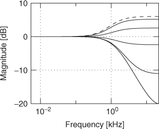
The overall magnitude responses of the block responsible for head shadowing is reported in Figure 5.3.

Figure 5.3 Magnitude responses of the simplified HRTFs for the ear in negative azimuth side. Azimuth ranging from (dashed line) to at steps of π/6.

The M-file implementing the head-shadowing filter as a time-domain HRIR is:

The function simpleHRIR gives a rough approximation of HRIR of one ear with one direction. To obtain a HRIR for the left and right ears the same function has to be used with opposite values of argument theta. An example is presented in Section 5.4.3.

5.4.3 HRTF Processing for Headphone Listening

A monophonic sound signal can be positioned virtually in any direction in headphone listening, if HRTFs for both ears are available for the desired virtual source direction [MSHJ95, Beg94]. The result of the measurements is a set of HRIRs that can be directly used as coefficients of a pair of FIR filters. Since the decay time of the HRIR is always less than a few milliseconds, 256 to 512 taps are sufficient at a sampling rate of 44.1 kHz. A sound signal is filtered with a digital filter modeling the measured HRTFs. The method simulates the ear-canal signals that would have been produced if a sound source existed in a desired direction.

A point-like virtual source is created with this example:

The demonstration above produces very probably the perception of inside-head virtual source, which may also sound colored. If a head tracker is available, much more realistic perception of external sound sources can be obtained with headphones. In head tracking, the direction of the listener's head is monitored about 10–100 times a second, and the HRTF filter is changed dynamically to keep the perceived direction of sound constant with the space where the listener is. In practice, the updating of the HRTF filter has to be done carefully in order not to produce audible artifacts.

The technique discussed above simulates anechoic listening of a distant sound source. It is also possible to simulate with the same technique the binaural listening of a sound source in a real room. In this approach, the binaural room impulse responses (BRIRs) are measured from the ear canals of a subject in a room with a relatively distant loudspeaker. The main difference to HRTFs is that typically the lengths of HRTFs are of the order of a few milliseconds and include only the acoustical response of the subject, whereas the BRIRs include the room responses, and they can be even few seconds long. The same MATLAB® example can also be used to process sound with BRIRs, although the required processing is much heavier in that case, since the convolution with such long responses is computationally a complex process.

HRTFs can also be used for cross-talk-canceled loudspeaker listening. In that case, the binaural signals are computed as shown in this section, and then played back with a stereo dipole, as shown in Section 5.4.5.

5.4.4 Virtual Surround Listening with Headphones

An interesting application for HRTF technologies with headphones is listening to existing multichannel audio material. In such cases, each loudspeaker in the multichannel loudspeaker layout is simulated using an HRTF pair. For example, a signal meant to be applied to the loudspeaker in a 30° direction is convolved with the HRTF pair measured from the same direction, and the convolved signals are applied to the headphones. The usage of HRTFs measured in anechoic conditions is often suboptimal in this case, and the use of BRIRs is beneficial, which have similar responses to the room in which the subject is located. This can be done using measured room impulse responses, or by simulating the effect or room with a reverberator, see Section 5.6.

An example of virtual loudspeaker listening with headphones:

5.4.5 Binaural Techniques with Cross-talk Canceled Loudspeakers

Binaural recordings are meant to be played back in such a way that the sound which originates from the left ear is played back only to the left ear, and correspondingly with the right ear. If such a recording is played back with stereophonic setup of loudspeakers, the sound from the left loudspeaker also travels to the right ear, and vice versa, called cross-talk, which ruins the spatial audio quality.

In order to be able to listen to binaural recordings over two loudspeakers, some methods have been proposed [CB89, KNH98]. In these methods, the loudspeakers are driven in such a way that in practice the cross-talk is canceled as much as possible.

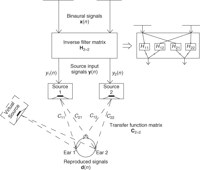
A system can be formed as presented in Figure 5.4 to deliver binaurally recorded signals to the listener's ears using two closely spaced loudspeakers with cross-talk cancellation. The binaural signals are represented as a 2x1 vector in x(n), and the produced ear canal signals also as 2x1 vector d(n). The system can be formulated in the z-domain

5.10

where contains the electro-acoustical responses of the loudspeakers measured in the ear canals, as shown in the figure, and contains the responses for performing inverse filtering to minimize the cross-talk.

Figure 5.4 Presentation of binaurally recorded signals with loudspeakers with cross-talk canceling [Pol07].

Ideally, x(z) = d(z), which can be obtained if H(z) = C(z)−1. Unfortunately, the direct inversion is not feasible due to unidealities of the loudspeakers and the listening conditions. A regularized method to find an optimal Hopt(z) has been proposed in [KNH98],

5.11

where β is a positive scalar regularization factor, and z−m models the time delay due to the sound reproduction system. If β is selected very low, there will be sharp peaks in the resulting time-domain inverse filters, which may exceed the dynamic range of the loudspeakers. If β is selected to be higher, the inverse filter will have longer duration in time, which is less demanding on the loudspeakers, but unfortunately the inversion is also less accurate [KNH98].

A MATLAB example is provided in the following to compute inverse filters for a cross-talk canceling system:

• The responses in C are moved into the frequency domain with discrete Fourier transform (DFT) with the desired length of time window.
• The filter responses are computed by where k presents the frequency bin indexes and H Hermitian transposition.
• The inverse DFT is taken of H, resulting in the inverse filters for cross-talk cancellation.
• A circular shift of half of the applied time-window length is implemented on the inverse filters.

In practice, this method works best with loudspeakers close to each other, as a larger loudspeaker base angle would lead to coloration at lower frequencies. The listening area in which the effect is audible is very small, as if the listener departs from the mid line between the loudspeakers by about 1–2 cm, the effect is lost.

A nice feature of this technique is that the sound is typically externalized. This may be due to the fact that head movements of the listener produce somewhat relevant cues, and since the sound is reproduced using far-field loudspeakers generating plausible monaural spectral cues. However, although the sound is externalized, a surrounding spatial effect is hard to obtain with this technique. With a stereo dipole in the front, the reproduced sound scene is typically perceived only at the front.

The technique also is affected by the reflections and reverberation of the listening room. It works best only in spaces without prominent reflections. To get the best results, the HRTFs of the listener should be known, however already very plausible results can be obtained with generic responses.