6.5 Time Shuffling and Granulation

6.5.1 Time Shuffling

Introduction

Musique concrète has made intensive use of splicing of tiny elements of magnetic tape. When mastered well, this assembly of hundreds of fragments of several tens of milliseconds allows an amalgamation of heterogeneous sound materials, at the limit of the time discrimination threshold. This manual operation, called micro-splicing, is very time-consuming. Bernard Parmegiani suggested in 1980 at the Groupe de Recherches Musicales (GRM) that this could be done by computers. An initial version of the software was produced in the early 80s. After being rewritten, improved and ported several times, it was eventually made available on personal computers in the form of a program called brassage in French that will be translated here as time shuffling [Ges98, Ges00].

Signal Processing

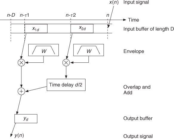
Let us describe here an elementary algorithm for time shuffling that is based on the superposition of two time segments that are picked randomly from the input signal (see Figure 6.22):

Figure 6.22 Time shuffling: two input segments, selected at random from the past input signal, are overlap-added to produce an output time segment. When one of the input segments is finished, a new one is selected.

Musical Applications and Control

The version described above introduces local disturbances into the signal's actual timing, while preserving the overall continuity of its time sequence. Many further refinements of this algorithm are possible. A random amplitude coefficient could be applied to each of the input segments in order to modify the density of the sound material. The shape of the envelope could be modified in order to retain more of the input time structure or, on the other hand, to smooth it out and blend different events with each other. The replay speed of the segments could be varied in order to produce transposition or glissandi.

At a time when computer tools were not yet available, Bernard Parmegiani magnificently illustrated the technique of tape-based micro-splicing in works such as “Violostries” (1964) or “Dedans-Dehors” (1977) [m-Par64, m-Par77]. The elementary algorithm presented above can be operated in real time, but other off-line versions have also been implemented which offer many more features. They have the ability to merge fragments of any size, sampled from a random field, and of any dimension; from a few samples to several minutes. Thus, apart from generating fusion phenomena, for which the algorithm was conceived, the software was able to produce cross-fading of textured sound and other sustained chords, infinitely small variations in signal stability, interpolation of fragments with silence or sounds of other types [Ges98]. Jean-Claude Risset used this effect to perform sonic developments from short sounds, such as stones and metal chimes [m-INA3, Sud-I, 3'44'' to 4'38'']; [Ris98, Ges00] and to produce a “stuttering” piano, further processed by ring modulation [m-INA3, Sud-I, 4'30'', 5'45'']. Starting from “found objects” such as bird songs, he rearranged them in a compositional manner to obtain first a pointillistic rendering, then a stretto-like episode [m-INA3, Sud-I, 1'42'' to 2'49''].

6.5.2 Granulation

Introduction

In the previous sections about pitch shifting and time stretching we have proposed algorithms that have limitations as far as their initial purpose is concerned. Beyond a limited range of modification of pitch or of time duration, severe artifacts appear. The time-shuffling method considers these artifacts from an artistic point of view and takes them for granted. Out of the possibilities offered by the methods and by their limitations, it aims to create new sound structures. Whereas the time-shuffling effect exploits the possibilities of a given software arrangement, which could be considered here as a “musical instrument,” the idea of building a complex sound out of a large set of elementary sounds could find a larger framework.

The physicist Dennis Gabor proposed in 1947 the idea of the quantum of sound, an indivisible unit of information from the psychoacoustical point of view. According to his theory, a granular representation could describe any sound. Granular synthesis was first suggested as a computer music technique for producing complex sounds by Iannis Xenakis (1971) and Curtis Roads (1978). This technique builds up acoustic events from thousands of sound grains. A sound grain lasts a brief moment (typically 1 to 100 ms), which approaches the minimum perceivable event time for duration, frequency and amplitude discrimination [Roa96, Roa98, Tru00a].

The granulation effect is an application of granular synthesis where the material out of which the grains are formed is an input signal. Barry Truax has developed this technique [Tru88, Tru94] by first real-time implementation and using it extensively in his compositional pieces.

Signal Processing

Let x(n) and y(n) be the input and output signals. The grains gk(i) are extracted from the input signal with the help of a window function wk(i) of length Lk by

6.6

with i = 0, …, Lk−1. The time instant ik indicates the point where the segment is extracted; the length Lk determines the amount of signal extracted; the window waveform wk(i) should ensure fade-in and fade-out at the border of the grain and affects the frequency content of the grain. Long grains tend to maintain the timbre identity of the portion of the input signal, while short ones acquire a pulse-like quality. When the grain is long, the window has a flat top and is used only to fade-in and fade-out the borders of the segment.

The following M-files 6.6 and 6.7 show the extraction of short and long grains:

The synthesis formula is given by

6.7

where ak is an eventual amplitude coefficient and nk is the time instant where the grain is placed in the output signal. Notice that the grains can overlap. To overlap a grain gk (grain) at instant nk = (iniOLA) with amplitude ak, the following MATLAB instructions can be used

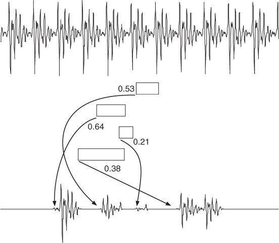
An example of granulation with random values of the parameters grain initial point and length, output point and amplitude is shown in Figure 6.23. The M-file 6.8 shows the implementation of the granulation algorithm.

Figure 6.23 Example of granulation.

This technique is quite general and can be employed to obtain very different sound effects. The result is greatly influenced by the criterion used to choose the instants nk. If these points are regularly spaced in time and the grain waveform does not change too much, the technique can be interpreted as a filtered pulse train, i.e., it produces a periodic sound whose spectral envelope is determined by the grain waveform interpreted as an impulse response. An example is the PSOLA algorithm shown in the previous Sections 6.3.3 and 6.4.4. When the distance between two subsequent grains is much greater than Lk, the sound will result in grains separated by interruptions or silences, with a specific character. When many short grains overlap (i.e., the distance is less than Lk), a sound texture effect is obtained.

The strategies for choosing the synthesis instants can be grouped into two rather simplified categories: synchronous, mostly based on deterministic functions, and asynchronous, based on stochastic functions. Grains can be organized in streams. There are two main control variables: the delay between grains for a single stream, and the degree of synchronicity among grains in different streams. Given that the local spectrum affects the global sound structure, it is possible to use input sounds that can be parsed in grains without altering the complex characteristics of the original sound, as water drops for stream-like sounds.

It is further possible to modify the grain waveform with a time transformation, such as modulation for frequency shifting or time stretching for frequency scaling [DP91]. The main parameters of granulation are: grain duration, selection order from input sound, amplitude of grains, temporal pattern in synthesis and grain density (i.e., grains per second). Density is a primary parameter, as it determines the overall texture, whether sparse or continuous. Notice that it is possible to extract grains from different sound files to create hybrid textures, e.g., evolving from one texture to another.

Musical Applications

Examples of the effect can be found in [m-Wis94c]. Barry Truax has used the technique of granulation to process sampled sound as compositional material. In “The Wings of Nike” (1987) he has processed only short “phonemic” fragments, but longer sequences of environmental sound have been used in pieces such as “Pacific” (1990). In each of these works, the granulated material is time stretched by various amounts and thereby produces a number of perceptual changes that seem to originate from within the sound [Tru00b, m-Tru95].

In “Le Tombeau de Maurice,” Ludger Brümmer uses the granulation technique in order to perform timbral, rhythmic as well as harmonic modifications [m-Bru97]. A transition from the original sound color of an orchestral sample towards noise pulses is achieved by reducing progressively the size of the grains. At an intermediate grain size, the pitch of the original sound is still recognizable, although the time structure has already disappeared [m-Bru97, 3'39''-4'12'']. A melody can be played by selecting grains of different pitches and by varying the tempo at which the grains are replayed [m-Bru97, 8'38''-9'10'']. New melodies can even appear out of a two-stage granulation scheme. A first series of grains is defined from the original sample, whereas the second is a granulation of the first one. Because of the stream segregation performed by the hearing system, the rhythmic as well as the harmonic grouping of the grains is constantly evolving [m-Bru97, 9'30''-10'33''].