
Chapter 15. Scaling Out
Distributing for scale and replicating for availability both rely on multiple instances of every node running on separate computers. But as computers can (and will) end up missing in action and connectivity among them will fail, scaling out is not only about adding computing capacity. Rather, scaling out must be carefully integrated and orchestrated with your consistency and availability models, where you have already chosen which tradeoffs to make. It’s easy to say that you need to write a system that scales infinitely without losing a single request, but delivering it is never simple, and it’s often the case that such an ideal implementation is unnecessary in practice to support your target applications. While Erlang/OTP systems do not scale magically, using OTP and making the right tradeoffs takes a large part of the pain out of the process.
In this chapter, we follow on from the distributed programming patterns and recovery and data-sharing patterns described in Chapter 13 and Chapter 14, focusing on the scalability tradeoffs you make when designing your architecture. We describe the tests needed to understand your system’s limitations and ensure it can handle, without failing, the capacity for which it was designed. This allows you to put safeguards in place, ensuring users do not overflow the system with requests it can’t handle. The last thing you want to deal with when under heavy load is a node crash, the degradation of throughput, or a service provider or third-party API not responding as a result of the wrath of Erlang being unleashed upon it.
Horizontal and Vertical Scaling
The scalability of a system is its ability to handle changes in demand and behave predictably, especially under spikes or sustained heavy loads. Scalability can be achieved vertically, by throwing more powerful computers at the problem, or horizontally, by adding more nodes and hardware.
Vertical scalability, also referred to as scaling up, might at first glance appear to be a quick win. You have a single server that guarantees strong consistency of your data. You just add larger chips, faster clock cycles, more cores and memory, a faster disk, and more network interfaces. Who does not like the feeling of opening a box containing the fastest, shiniest, highest capacity, yet slimmest computer on which to benchmark your software?
But alas, this approach is dated, because servers can only get so big, and the bigger they get, the more expensive they become. And you need at least two, because a super fast computer can still be a single point of failure.
Another argument for scaling horizontally is multicore. With machines supporting thousands of cores, no matter how parallel and free of bottlenecks your program might be, there are only so many cores a single VM will be able to optimally utilize. You need to also keep in mind that Amdahl’s Law applies not only to your Erlang program, but to the sequential code in the Erlang VM. This likely means that in order to fully utilize the hardware, you have to run multiple distributed VMs on a single computer. If you need to deal with two computers or computers running multiple Erlang nodes, you might as well take the leap and scale horizontally.
Scaling horizontally, also known as scaling out, is achieved using cloud instances and commodity hardware. If you need more processing power, you can rent, buy, or build your own machines and deploy extra nodes on them. Distributed systems, whether you want them or not, are your only viable approach. They will scale better, are much more cost-effective, and help you achieve high availability. But as we have seen in the previous chapters, this will require rethinking how you architect your applications.
In small clusters running distributed Erlang, Erlang/OTP scales vertically or horizontally in essentially the same way. In both cases, scaling is achieved using the location transparency of processes, meaning they act the same way whether they run locally or remotely. Processes communicate with each other using asynchronous message passing, which in soft real-time systems absorbs at the cost of latency across nodes. And asynchronous error semantics also work across nodes. As a result, a system written to run on a single machine can easily be distributed across a cluster of nodes. This also facilitates elasticity, the ability to add and remove nodes (and computers) at runtime so you can cater not only for failure, but also for peak loads and systems with a growing user base.
Capacity Planning
Understanding what resources your node types use and how they interact with each other allows you to optimize the hardware and infrastructure in terms of both efficiency and cost. This work is called capacity planning. Its purpose is to try to guarantee that your system can withstand the load it was designed to handle, and, with time, scale to manage increased demand.
The only way to determine the load and resource utilization and balance the required number of different nodes working together is to simulate high loads, testing your system end to end. This ensures the nodes are able to work together under extended heavy load, handling the required capacity in a predictable manner without any bottlenecks. It also allows you to test your system’s behavior in case of failure.
In Chapter 13, we suggest you divide your system functionality into node types and families and connect nodes in a cluster. Although one can argue that grouping the different applications of all your node types together—front-end, business logic, and service functionality in the same node—will run fast because everything is running in the same memory space, this solution is not recommended for anything other than simple systems. For complex systems, it is easier to divide and conquer, studying and optimizing throughput and resource utilization on nodes that are limited in functionality.
Balancing your system is also a cost optimization exercise, where you try to reduce the costs of hardware, operations, and maintenance. Imagine front-end nodes that parse relatively few simultaneous requests, but act as an interface to clients who keep millions of TCP connections open. These nodes will most likely be memory-bound and need a different type of hardware specification from a CPU-bound front-end node that has fewer, but more traffic-intensive, connections and spends most of its time parsing and generating JSON or XML. Logic nodes routing requests and running computationally intensive business logic will need more cores and memory, while a service node managing a database will probably be I/O-bound and need a fast hard disk.
An often overlooked item when dealing with capacity planning is ensuring you can handle the designated load even after a software, hardware, or network failure. If your system has two front-end nodes for every logic node and both run at 100% memory or CPU capacity, losing a front-end node means you will now be able to handle only half of your designated load. To ensure you have no single point of failure, you need at least three front-end nodes running at a maximum capacity of 66% CPU each and two back-end nodes averaging 50% CPU each. This way, losing any machine or node will still guarantee you can handle your peak load requirements. If you want triple redundancy, you will have to throw even more hardware at the problem.
When working with capacity planning, you will be measuring and optimizing your system in terms of throughput and latency. Throughput refers to the number of units going through the system. Units could be measured in number of requests per second when dealing with uniform requests, but when the CPU load and amount of memory needed to process the requests vary in size (think emails or email attachments), throughput is better measured in kilobytes, megabytes, or gigabytes per second.
Latency is the time it takes to serve a particular request. Latency might vary depending on the load of your system, and is often correlated to the number of simultaneous requests going through it at any point in time. More simultaneous requests often means higher latency.
The predictable behavior of the Erlang runtime system, where a balanced system under heavy load results in a constant throughput, addresses most use cases. But there might be instances where extreme usage spikes or third-party services that are slow in responding could result in a backlog of requests, an outage caused by the Erlang VM running out of system resources, or the need to apply load regulation so latency stays within predefined intervals.
In “Tradeoffs Between Consistency and Availability”, we discussed the tradeoffs between consistency and availability based on your recovery and data-sharing strategies and distributed architectural patterns. You might not have realized it, but you were also making tradeoffs with scalability (Figure 15-2).
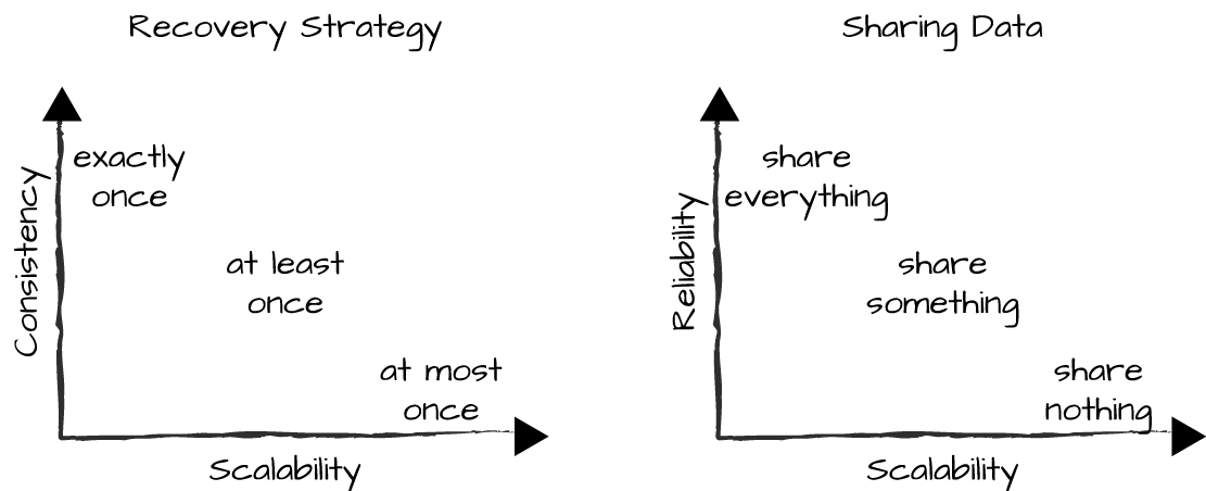
Figure 15-2. Scalability tradeoffs
The most scalable framework is SD Erlang. With it, you effectively share data within an s_group, but minimize what is shared across s_groups. Data and workflows shared among s_groups go through gateway nodes. By controlling the size of s_groups and the number of gateways, you can have strong consistency within an s_group and eventual consistency among s_groups.
Riak Core comes second, and despite being a fully meshed Erlang cluster, it can scale well by using consistent hashing to shard your data and load balancing jobs across the cluster. You can use it as a giant switch running your business logic, connecting service nodes that are part of the cluster, but not fully meshed to the core itself. With a hundred connected nodes in the core, where each node handles thousands of requests per second, most seriously scalable event-driven systems should fall under this category. Thanks to vnodes, you can start small and minimize disruption when nodes are added (or removed).
Lastly, a distributed Erlang cluster is limited in scale but does well enough to cater to the vast majority of Erlang systems. Even if you are aiming for tens of thousands of requests per second, you will often find it is more than enough. Be realistic in your capacity planning and add complexity only when you need it.
On one end of the scale are the exactly-once and share-everything approaches, which lean toward consistency and reliability, respectively. They are also the most expensive in terms of CPU power and network requirements, and as such, are also the least scalable. If you want a truly scalable system, you need to reduce the amount of shared data to a minimum and, if you have to share data, use eventual consistency wherever appropriate. Use asynchronous message passing across nodes, and in cases where you need strong consistency, minimize it in as few nodes as possible, placing them close to each other so as to reduce the risk of network failure.
Capacity Testing
Capacity testing is a must when working with any scalable and available system to help ensure its stability and understand its behavior under heavy load. This is true regardless of what programming language you use to code the system.
What is your system’s maximum throughput before it breaks? How is the system affected by increased utilization or the loss of a computer resulting from a hardware or network malfunction? And is the latency of these requests under different loads acceptable? You need to ensure your system remains stable under extended heavy load, recovers from spikes, and stays within its allocated system limits. Too often, systems are deployed without any proper stress testing, and they underperform or crash under minimal load because of misconfiguration or bottlenecks. To reduce the risk of running into these issues when going live, you will have to apply the four testing strategies shown in Figure 15-3.
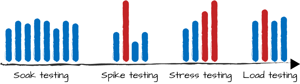
Figure 15-3. Capacity-testing strategies
They are:
- Soak testing
This generates a consistent load over time to ensure that your system can keep on running without any performance degradation. Soak tests can continue for months and are used to test not only your system, but the whole stack and infrastructure.
- Spike testing
This ensures you can handle peak loads and recover from them quickly and painlessly.
- Stress testing
This gradually increases the load you are generating until you hit bottlenecks and system limits. Bottlenecks are backlogs in your system whose symptom is usually long message queues. System limits include running out of ports, memory, or even hard disk space. When you have found a bottleneck and removed it, rerun the stress test again to tackle the next bottleneck or system limit.
- Load testing
This pushes your system at a constant rate close to its limits, ensuring it is stable and balanced. Run your load test for at least 24 hours to ensure there is no degradation in throughput and latency.
Don’t underestimate the time, budget, and resources it takes to remove bottlenecks and achieve high throughput with predictable latency. You need hardware to generate the load, hardware to run your simulators, and hardware to run multiple tests in parallel. With crashes that take days to generate, running parallel tests with full visibility of what is going on is a must. It will at times feel like you are looking for a needle in a haystack as you are troubleshooting and optimizing your software stack, hardware, and network settings.
Generating load
How you generate load varies across systems and organizations. You can use existing open source tools and frameworks such as Basho Bench, MZBench, and Tsung; commercial products; or SaaS load-testing services. Some tools allow you to record and replay live traffic. Or if you want to simulate complex business client logic or test simple scenarios, it might be easier to write your own tests. You will soon discover that to test an Erlang system, you will most likely need a load tool written in Erlang.
If you are connecting to third-party services or want to test node types on a stand-alone basis, you will need to write simulators, because your third parties will most likely not allow you to test against live systems. Simulators like the one shown in Figure 15-4 are often standalone Erlang nodes that expose the external API and, to some degree of intelligence, replicate their behavior. They are designed to handle the load of your external services, but often go far beyond that.
Warning
Exercise extreme care when load testing the final instance of your system right before going live, and make sure you are connected to your simulators and have throttling in place toward your external service providers. We would advise against you discovering the hard way that your external service providers do not have any load control in place. We once ran load tests on an autodialer we were writing, forgetting to divert the requests to the simulators. The error caused a major outage of the IP telephony provider we were planning to use. They were not too happy. Nor were we, as we got kicked out and had to find and integrate with a new provider days before going live.
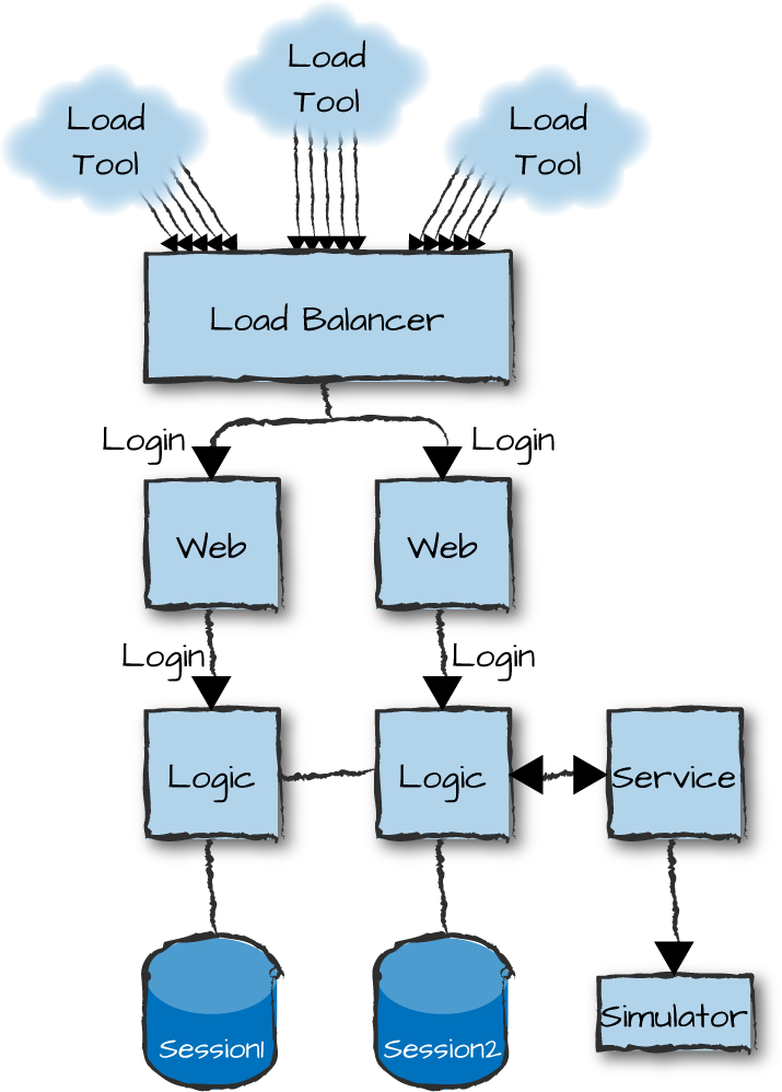
Figure 15-4. An Erlang system under load
Balancing Your System
In a properly balanced Erlang system running at maximum capacity, the throughput should remain constant while latency varies. If the work cost per request is constant and your system handles a peak throughput of 20,000 requests per second, when 20,000 requests are going through the system at any one time, the peak latency should be 1 second. If 40,000 requests are going through the system simultaneously, it will take the system 2 seconds to service a request. So, while throughput remains the same—20,000 requests per second—the latency doubles. The BEAM VM is one of the few virtual machines to display this property, providing predictability for your system even under sustained extreme loads.
In Figure 15-5 we show a graph where the y-axis represents the throughput of a typical Erlang system before being optimized. It could be the number of instant messages handled per second, the throughput in megabytes of data sent by a web server, or the number of log entries being formatted and stored to file. The x-axis shows the number of simultaneous requests going through the system at any one time. This degradation often manifests itself after hitting high CPU loads. At that point, the more requests there are going through the system, the lower the throughput and higher the latency. It is important that you understand this behavior of the BEAM virtual machine, as it is bound to affect you.
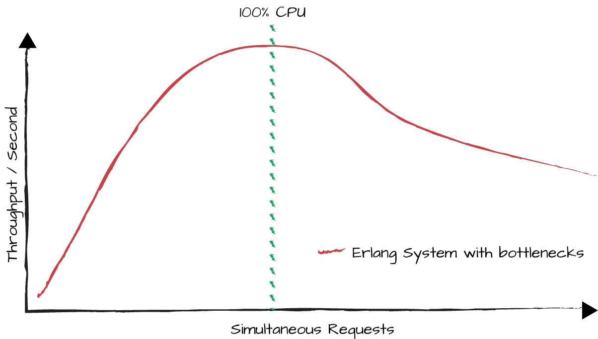
Figure 15-5. Degradation of an Erlang system under load
Line 2 in Figure 15-6 shows the result of removing bottlenecks in the system. You should get a constant throughput regardless of the number of simultaneous requests. The throughput at peak load might go down a little, but that is a small price to pay for a system that will behave in a predictable manner irrespective of the number of simultaneous requests going through it. Most other languages will experience degraded throughput because processes have high context-switching costs. Using the Erlang virtual machine, highly optimized for concurrency, greatly reduces the risk. The limit on how much a node can scale is now determined by system limits such as CPU load, available memory, or I/O. We refer to nodes hitting these limits as being CPU-bound, memory-bound, or I/O-bound. The shared area shows the performance degradation of a badly balanced system.
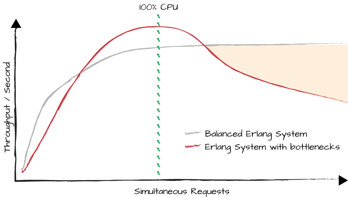
Figure 15-6. An Erlang system tuned to handle large loads
To find the bottlenecks in your system, start off testing a single node. Use simulators, but be wary of premature optimizations. Some node types might not need to be optimized, as they might never be subjected to heavy loads. And you might end up with nodes that are super fast, but continue to respond too slowly because service-level agreements with external APIs now become your bottleneck. The goals of your various capacity testing exercises are to measure and record how latency, throughput, and simultaneous requests going through the system affect one another.
In some cases, bottlenecks will throttle requests that surprisingly keep the service alive. The problem is that they tend to slow it down. For this reason, it sometimes makes sense to test your system on different hardware and VM configurations.
Consider your system stable only when all performance bottlenecks have been removed or optimized, leaving you to deal with issues arising from your external dependencies such as I/O, your filesystem, or network or external third-party services not being able to handle your load. These items are often out of your control, leaving it necessary to regulate your loads instead of continuing to scale up or out.
Finding Bottlenecks
When you are looking for bottlenecks on a process and node basis, most
culprits are easily found by monitoring process memory usage and mailbox
queues. Memory usage is best monitored using the
erlang:memory() BIF, which returns a list of tuples with
the dynamic memory allocations for processes, ETS tables, the binary
heap, atoms, code, and other things.
You need to monitor the different categories of memory usage
throughout your load testing, ensuring that there are no leaks and that
resource usage is constant for long runs. If you see the atom table or
binary heap increasing in size over time without stabilizing, you might
run into problems days, weeks, or months down the line. At some point,
you will also want to use the system monitor, described in “The System Monitor”, to ensure that process memory spikes and
long garbage collections are optimized or removed. Message queues can be
monitored using the i() or regs() shell
commands.
If using the shell is not viable because you are working with millions of processes, the percept and etop tools will often work, as might the observer tool. Along with other monitoring tools, we discuss collecting system metrics in “Metrics”. If you are collecting system metrics and feeding them into your OAM infrastructure, you can use them to locate and gain visibility into bottlenecks.
The biggest challenge, however, is often not finding the
bottlenecks, but creating enough load on your system to generate them.
Multicore architectures have made this more difficult, as huge loads will
often expose issues in other parts of the stack that are related not to
Erlang, but to the underlying hardware, operating system, and
infrastructure. One approach to detecting some of your bottlenecks is to
run your Erlang virtual machine with fewer cores using the erl
+S flag, or stress testing the node on less powerful hardware.
Synchronous versus asynchronous calls
Most commonly, bottlenecks manifest themselves through long message
queues. Imagine a process whose task is to format and store logs to
files. Assume that for every processed request we want to store dozens
of log entries. We start sending our log requests asynchronously using
gen_server:cast to a log server that can’t cope with the
load, because each request process is generating log entries at a rate
faster than what the generic server process can handle. Multiply that
by thousands of producers and slow file I/O, and you’ll end up with a
huge message queue in the consumer’s mailbox. This queue is the
manifestation of a bottleneck that negatively affects the behavior of
your system. How does this happen?
Every operation in your program is assigned a number of
reductions (covered in “Multicore, Schedulers, and Reductions”), each of which
is roughly equivalent to one Erlang function call. When the scheduler
dispatches a process, it is assigned a number of reductions it is
allowed to execute, and for every operation, it reduces the reduction
count. The process is suspended when it reaches a receive
clause where none of the messages in the mailbox match, or the
reduction count reaches zero. When process mailboxes grow in size, the
Erlang virtual machine penalizes the sender process by increasing the
number of reductions it costs to send the message. It does so in an
attempt to control producers and allow the consumer to catch up. It is
designed this way to give the consumer a chance to catch up after a
peak, but under sustained heavy load, it will have an adverse effect
on the overall throughput of the system. This scenario, however,
assumes there are no bottlenecks. Penalizing senders with added
reductions is not adequate to prevent overgrown message queues for
overloaded processes.
A trick to regulate the load and control the flow, so as to get
rid of these bottlenecks, is to use synchronous calls even if you do
not require a response back from the server. When you use a
synchronous call, a producer initiating a request will not send a new
log request until the previous one has been received and acknowledged.
Synchronous calls block the producer until the consumer has handled
previous requests, preventing its mailbox from being flooded. It will
have the same effect described in Figure 15-6,
where, at the expense of throughput, you get a stable and predictable
system. When using this approach, remember to fine-tune your timeout
values, never taking the default 5-second value for granted, and never
setting it to infinity.
Another strategy for reducing bottlenecks is to reduce the workload in the consumers, moving it where possible to the clients. In the case of log entries, for example, you could process them in batches, flushing a couple hundred of them at a time to disk. You could also offload work to the requesting process, making it format the entries instead of leaving that to the server. After all, formatting log entries can be done concurrently, whereas writing the log entries to disk must take place sequentially.
Now that you’ve optimized your code, learned your system’s limits, and addressed its bottlenecks, you will need guarantees that your system will not fail over or degrade in performance if you hit those limits.
System Blueprints
If you have come this far, the time has come to formalize all your design choices into cluster and resource blueprints, combining them together into a system blueprint. Your resource blueprint specifies the available resources on which to run your cluster. It includes descriptions of hardware specifications or cloud instances, routers, load balancers, firewalls, and other network components.
Your cluster blueprint is derived from the lessons learned from your capacity planning. It is a logical description of your system, specifying node families and the connectivity within and among them. You also define the ratios of different node types you need to have a balanced system capable of functioning with no degradation of service. This blueprint can be used by your orchestration programs to ensure your cluster can be scaled in an orderly fashion, without creating imbalances among your nodes. It should also ensure your system can continue running after failure, with no degradation of service. Cluster blueprints are analogous to an Amazon autoscaling group on Amazon Web Services, but are more detailed. When you hit an upper limit in one of your clusters, deploy a new cluster.
Your cluster and resource blueprints are combined in what we call a system blueprint. With the system blueprint in hand, you can understand both how your distributed system is structured and how it can be deployed on hardware or cloud instances.
Load Regulation and Backpressure
A long, long time ago, on New Year’s Eve, in a country far, far away, everyone picked up the phone and called to wish one another a happy and prosperous new year. Phone trunks were jammed. Calls were allowed through at the rate the various trunks were configured to handle, and the network kept on operating despite the surge. It behaved predictably for the maximum capacity it was designed to manage.
The system stayed afloat because it employed backpressure to limit the number of connected calls made through a trunk at any point in time. You always got the dial tone and were allowed to dial, but if you tried to access an international trunk with no available lines, your call was rejected with a busy tone. So you kept on trying until you got through. Backpressure is the approach of telling the sender to stop sending because there’s no room for new messages.
From phone calls, the world moved to SMSs. As SMS became popular, the spike on New Year’s Eve started getting larger, as did the delays in delivering the SMSs. And as soon as mobile phones allowed you to send SMSs in bulk to dozens of users, delays got even worse, with messages often arriving in the early hours of the morning when their senders (and recipients) had long since gone to bed. Rarely were SMSs rejected—they got through, but with major delays. The mobile operators were applying a technique called load regulation, where the flow of requests was diverted to a queue to ensure that no requests were lost. Messages were retrieved from the queue and sent to the SMS center (SMSC) as fast as it could handle them.
Calling each other or sending SMSs might be a thing of the past, but the techniques developed and used in the telecom space still remain relevant when dealing with massive scale. Together, load regulation and backpressure allow you to keep throughput and latency predictable while ensuring your system does not fail as a result of overload. The difference is that load regulation allows you to keep and remember requests by imposing limits on the number of simultaneous connections and throttling requests using queues, while backpressure rejects them. If you are using load regulation toward third-party APIs or service nodes, remember that all you are doing is smoothing out your peaks and troughs, ensuring you do not overflow the third party with requests. If you keep on receiving requests at a rate faster than they can handle, you will eventually have to stop queuing and start rejecting.
Let’s use our New Year’s Eve SMS example. If the gateway is receiving more texts than can be handled by the SMSC (which forwards texts to your mobile terminal), it queues the texts in your load-regulation application, feeding them on a FIFO basis at the rate the SMSC can handle. This rate is called the service-level agreement. If the SMSs keep on coming in at this fast rate for a sustained period of time, the queue size is bound to hit its limit and overflow. When this happens, the gateway starts rejecting SMSs, either individually in the logic nodes or in bulk by triggering some form of backpressure in the front-end nodes, and not accepting them in the gateway nodes. This scenario is illustrated in Figure 15-7.
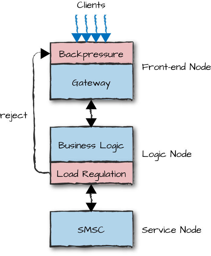
Figure 15-7. Load regulation and backpressure
In order to throttle requests and apply backpressure, you need to use load-regulation frameworks. These could be embedded into your Erlang nodes, or be found at the edges in the front-end and service nodes. Another common practice to control load is through load balancers. Software and hardware load balancers will, on top of balancing requests across front-end nodes, also throttle the number of simultaneously connected users and control the rate of inbound requests. Sadly, this will by default involve stress testing the load balancers themselves, opening a new can of worms.1 Whoever said it was easy to develop scalable, resilient systems?
Keep in mind that load regulation comes at a cost, because you are using queues and a dispatcher can become a potential bottleneck that adds overhead. Start controlling load only if you have to. When deploying a website for your local flower shop, what is the risk of everyone in town flocking to buy flowers simultaneously? If, however, you are deploying a game back end that has to scale to millions of users, load regulation and backpressure are a must. They give you the ability to keep the latency or throughput of your system constant despite peak loads, and ensure your system does not degrade in performance or crash as a result of hitting system limits. There are two widely used load-regulation applications in Erlang: Jobs and Safetyvalve.
Summing Up
In this chapter, we’ve covered the scalability aspects to take into consideration in Erlang/OTP-based systems. The key to the scalability of your system is ensuring you have loosely coupled nodes that can come and go. This provides elasticity to add computing power and scale on demand. You often want strong consistency within your nodes and node families and eventual consistency elsewhere. Communication should be asynchronous, minimizing guaranteed delivery to the subset of requests that really require it.
The steps to architecting your system covered in the previous two chapters included:
Split up your system’s functionality into manageable, standalone nodes.
Choose a distributed architectural pattern.
Choose the network protocols your nodes, node families, and clusters will use when communicating with each other.
Define your node interfaces, state, and data model.
For every interface function in your nodes, pick a retry strategy.
For all your data and state, pick your sharing strategy across node families, clusters, and types, taking into consideration the needs of your retry strategy.
Iterate through all these steps until you have the tradeoffs that best suit your specification. You will also have made decisions that directly impact scalability, resulting in tradeoffs between scalability, consistency, and availability. Now:
Design your system blueprint, looking at node ratios for scaling up and down.
To define your cluster and resource blueprints, you should understand how you are going to balance your front-end, logic, and service nodes based on your choice of distributed architectural patterns and target hardware. You need to remember the goal of no single point of failure, ensuring you have enough capacity to handle the required latency and throughput, and can achieve resilience even if you lose one of each node type. When you’re done, combine the two into a system blueprint.
The only way to validate your system blueprint is through capacity testing on target hardware. Write your simulators and run soak, stress, spike, and load tests to remove bottlenecks and validate your assumptions.
Identify where to apply backpressure and load regulation.
When capacity testing your system, you should strive to obtain a good idea of the system’s limitations. Understand where to apply load regulation and backpressure, protecting your system from degrading in performance or crashing altogether. How many simultaneous requests can go through the system before latency becomes too high or some nodes run out of memory? Is your system capable of handling failure with no degradation of service? Also, make sure you do not crash your third-party APIs and services, maintaining the accepted service-level agreements.
Our last word of advice is not to overengineer your system. Premature optimizations are the root of all evil. Do not assume you need a distributed framework, let alone use one just because it is there or because you can. Even if you’ll be writing the engine for the next generation of MMOGs or building the next WhatsApp, start small and ensure you get something that works end to end. Be prepared to use these frameworks, but hide them behind thin abstraction layers of software and APIs, allowing you to change your strategy at a later date. Then, when stress testing your system, recreate error scenarios. Kill nodes, shut down computers, pull out network cables, and learn how your system behaves and recovers from failure. During this stage you can decide what tradeoffs you will make between availability, consistency, and scalability. The difference in infrastructure cost between not losing any requests and losing the occasional one could mean an order of magnitude or more in hardware capacity. Do you really need 10 times more hardware, and the cost and complexity associated with it, for a service no one is paying for, and which very rarely fails anyhow?
What’s Next?
Now that you have a system that you believe is scalable, available, and reliable, you need to ensure your DevOps team has full visibility into what is happening on the system after it has gone live. In the next chapter, we cover metrics, logs, and alarms, which allow personnel supporting and maintaining the system to monitor it and take actions before issues escalate and get out of hand.
1 The sad part of this paragraph is that we’ve often caused load balancers to crash or behave abnormally and had to shut them down when load testing, because they weren’t powerful enough to withstand the load we were generating.