Recursion and Pattern Matching

Recursion is the way Erlang programmers get iterative or repetitive behavior in their programs. It is also what keeps processes alive in between bursts of activity. Our first example shows how to compute the factorial of a positive number:

-module(ex1).
-export([factorial/1]).

factorial(0) ->
    1;
factorial(N) when N > 0 ->
    N * factorial(N-1).

We call the function factorial and indicate that it takes a single argument (factorial/1). The trailing /1 is the arity of a function, and simply refers to the number of arguments the function takes—in our example, 1.

If the argument we pass to the function is the integer 0, we match the first clause, returning 1. Any integer greater than 0 is bound to the variable N, returning the product of N and factorial(N-1). The iteration will continue until we pattern match on the function clause that serves as the base case. The base case is the clause where recursing stops. If we call factorial/1 with a negative integer, the call fails as no clauses match. But we don’t bother dealing with the problems caused by a caller passing a noninteger argument; this is an Erlang principle we discuss later.

Erlang definitions are contained in modules, which are stored in files of the same name, but with a .erl extension. So, the filename of the preceding module would be ex1.erl. Erlang programs can be evaluated in the Erlang shell, invoked by the command erl in your Unix shell or by double-clicking on the Erlang icon. Make sure that you start your Erlang shell in the same directory as your source code. A typical session goes like this:

$ erl              % Comments on interactions are given in this format.
Erlang/OTP 18 [erts-7.2] [smp:8:8] [async-threads:10] [kernel-poll:false]

Eshell V7.2  (abort with ^G)
1> c(ex1).
{ok,ex1}
2> ex1:factorial(3).
6
3> ex1:factorial(-3).
** exception error: no function clause matching
                    ex1:factorial(-3) (ex1.erl, line 4)
4> factorial(2). 
** exception error: undefined shell command factorial/1
5> q().
ok
$

In shell command 1, we compile the Erlang file. We go on to do a fully qualified function call in command line 2, where by prefixing the module name to the function we are able to invoke it from outside the module itself. The call in shell command 3 fails with a function clause error because no clauses match for negative numbers. Before terminating the shell with the shell command q(), we call a local function, factorial(2), in shell command 4. It fails as it is not fully qualified with a module name.

Recursion is not just for computing simple values; we can write imperative programs using the same style. The following is a program to print every element of a list, separated by tabs. As with the previous example, the function is presented in two clauses, where each clause has a head and a body, separated by the arrow (->). In the head we see the function applied to a pattern, and when a function is applied to an argument, the first clause whose pattern matches the argument is used. In this example the [] matches an empty list, whereas [X|Xs] matches a nonempty list. The [X|Xs] syntax assigns the first element of the list, or head, to X and the remainder of the list, or tail, to Xs (if you have not yet noted it, Erlang variables such as X, Xs, and N all start with uppercase letters):

-module(ex2).
-export([print_all/1]).

print_all([]) ->
    io:format("~n");
print_all([X|Xs]) ->
    io:format("~p	",[X]),
    print_all(Xs).

The effect is to print each item from the list, in the order that it appears in the list, with a tab ( ) after each item. Thanks to the base case, which runs when the list is empty (when it matches []), a newline (~n) is printed at the end. Unlike in the ex1:factorial/1 example shown earlier, the pattern of recursion in this example is tail recursive. It is used in Erlang programs to give looping behavior. A function is said to be tail recursive if the only recursive calls to the function occur as the last expression to be executed in the function clause. We can think of this final call as a “jump” back to the start of the function, now called with a different parameter. Tail-recursive functions allow last-call optimization, ensuring stack frames are not added in each iteration. This allows functions to execute in constant memory space and removes the risk of a stack overflow, which in Erlang manifests itself through the virtual machine running out of memory.

If you come from an imperative programming background, writing the function slightly differently to use a case expression rather than separate clauses may make tail recursion easier to understand:¹

all_print(Ys) ->
    case Ys of
        [] ->
            io:format("~n");
        [X|Xs] ->
            io:format("~p	",[X]),
            all_print(Xs)
    end.

When you test either of these print functions, note the ok printed out after the newline. Every Erlang function has to return a value. This value is whatever the last executed expression returns. In our case, the last executed expression is io:format("~n"). The newline appears as a side effect of the function, while the ok is the return value printed by the shell:

1> c(ex2).
{ok,ex2}
2> ex2:print_all([one,two,three]).
one     two     three
ok
3> Val = io:format("~n").

ok
4> Val.
ok

The arguments in our example play the role of mutable variables, whose values change between calls. Erlang variables are single assignment, so once you’ve bound a value to a variable, you can no longer change that variable. In a recursive function variables of the same name, including function arguments, are considered fresh in every function iteration. We can see the behavior of single assignment of variables here:

1> A = 3.
3
2> A = 2+1.
3
3> A = 3+1.
** exception error: no match of right hand side value 4

In shell command 1, we successfully assign an unbound variable. In shell command 2, we pattern match an assigned variable to its value. Pattern matching fails in shell command 3, because the value on the right-hand side differs from the current value of A.

Erlang also allows pattern matching over binary data, where we match on a bit level. This is an incredibly powerful and efficient construct for decoding frames and dealing with network protocol stacks. How about decoding an IPv4 packet in a few lines of code?

-define(IP_VERSION, 4).
-define(IP_MIN_HDR_LEN, 5).

handle(Dgram) ->
   DgramSize = byte_size(Dgram),
   <<?IP_VERSION:4, HLen:4, SrvcType:8, TotLen:16, ID:16, ...,
     Flgs:3, FragOff:13, TTL:8, Proto:8,  HdrChkSum:16, ...,
     SrcIP:32, DestIP:32, Body/binary>> = Dgram,
   if
     (HLen >= 5) and (4*HLen =< DgramSize) ->
        OptsLen = 4*(HLen - ?IP_MIN_HDR_LEN),
        <<Opts:OptsLen/binary, Data/binary>> = Body,
        ...
   end.

We first determine the size (number of bytes) of Dgram, a variable holding an IPv4 packet as binary data previously received from a network socket. Next, we use pattern matching against Dgram to extract its fields; the left-hand side of the pattern matching assignment defines an Erlang binary, delimited by << and >> and containing a number of fields. The ellipses (...) within the binary are not legal Erlang code; they indicate fields we’ve left out to keep the example brief. The numbers following most of the fields specify the number of bits (or bytes for binaries) each field occupies. For example, Flgs:3 defaults to an integer that matches 3 bits, the value of which it binds to the variable Flgs. At the point of the pattern match we don’t yet know the size of the final field, Body, so we specify it as a binary of unknown length in bytes that we bind to the variable Data. If the pattern match succeeds, it extracts, in just a single statement, all the named fields from the Dgram packet. Finally, we check the value of the extracted HLen field in an if clause, and if it succeeds, we perform a pattern matching assignment against Body to extract Opts as a binary of OptsLen bytes and Data as a binary consisting of all the rest of the data in Body. Note how OptsLen is calculated dynamically. If you’ve ever written code using an imperative language such as Java or C to extract fields from a network packet, you can see how much easier pattern matching makes the task.

Functional Influence

Erlang was heavily influenced by other functional programming languages. One functional principle is to treat functions as first-class citizens; they can be assigned to variables, be part of complex data structures, be passed as function arguments, or be returned as the results of function calls. We refer to the functional data type as an anonymous function, or fun for short. Erlang also provides constructs that allow you to define lists by “generate and test,” using the analogue of comprehensions in set theory. Let’s first start with anonymous functions: functions that are not named and not defined in an Erlang module.

-module(ex3).
-export([filter/2, is_even/1]).

filter(P,[]) -> [];
filter(P,[X|Xs]) ->
    case P(X) of
        true ->
            [X|filter(P,Xs)];
        _ ->
            filter(P,Xs)
    end.

is_even(X) ->
    X rem 2 == 0.

2> ex3:filter(fun(X) -> X rem 2 == 0 end, [1,2,3,4]).
[2,4]
3> ex3:filter(fun ex3:is_even/1,[1,2,3,4]).
[2,4]

4> F = fun Filter(_,[]) -> [];
4> Filter(P,[X|Xs]) -> case P(X) of true -> [X|Filter(P,Xs)];
4> false -> Filter(P,Xs) end end.
#Fun<erl_eval.36.90072148>
5> Filter(fun(X) -> X rem 2 == 0 end,[1,2,3,4]).
* 1: variable 'Filter' is unbound
6> F(fun(X) -> X rem 2 == 0 end,[1,2,3,4]).
[2,4]

[Expression || Generators, Tests, Generators, Tests]

   X <- [2,3,5,7,11]

filter(P,Xs) -> [ X || X<-Xs, P(X) ].

1> [Element || Element <- [1,2,3,4], Element rem 2 == 0].
[2,4]
2> [Element || Element <- [1,2,3,4], ex3:is_even(Element)].
[2,4]
3> [Element || Element <- lists:seq(1,4), Element rem 2 == 0].
[2,4]
4> [io:format("~p~n",[Element]) || Element <- [one, two, three]].
one
two
three
[ok,ok,ok]

5> [ {X,Y} || X <- [1,2], Y <- [3,4,5] ].
[{1,3},{1,4},{1,5},{2,3},{2,4},{2,5}]
6> [ {X,Y} || X <- [1,2], Y <- [X+3,X+4,X+5] ].
[{1,4},{1,5},{1,6},{2,5},{2,6},{2,7}]
7> [ {X,Y} || X <- [1,2,3], X rem 2 /= 0, Y <- [X+3,X+4,X+5], (X+Y) rem 2 == 0 ].
[{1,5},{3,7}]
8> [ {X,Y} || X  <-[1,2,3], X rem 2 /= 0, Y <- [X+3,X+4,X+5], (X+Y) rem 2 /= 0 ].
[{1,4},{1,6},{3,6},{3,8}]

-module(queens).
-export([queens/1]).

queens(0) -> [[]];
queens(N) ->
    [[Row | Columns] || Columns <- queens(N-1),
        Row <- [1,2,3,4,5,6,7,8] -- Columns,	% -- returns the list difference
        safe(Row, Columns, 1)].

safe(_Row, [], _N) -> true;
safe(Row, [Column|Columns], N) ->
    (Row /= Column + N) andalso (Row /= Column - N) andalso
        safe(Row, Columns, (N+1)).

Processes and Message Passing

Concurrency is at the heart of the Erlang programming model. Processes are lightweight, meaning that creating them involves negligible time and memory overhead. Processes do not share memory, and instead communicate with each other through message passing. Messages are copied from the stack of the sending process to the heap of the receiving one. As processes execute concurrently in separate memory spaces, these memory spaces can be garbage collected separately, giving Erlang programs very predictable soft real-time properties, even under sustained heavy loads. Millions of processes can run concurrently within the same VM, each handling a standalone task. Processes fail when exceptions occur, but because there is no shared memory, failure can often be isolated as the processes were working on standalone tasks. This allows other processes working on unrelated or unaffected tasks to continue executing and the program as a whole to recover on its own.

So, how does it all work? Processes are created via the spawn(Mod, Func, Args) BIF or one of its variants. The result of a spawn call is a process identifier, normally referred to as a pid. Pids are used for sending messages, and can themselves be part of the message, allowing other processes to communicate back. As we see in Figure 2-1, the process starts executing in the function Func, defined in the module Mod with arguments passed to the Args list.

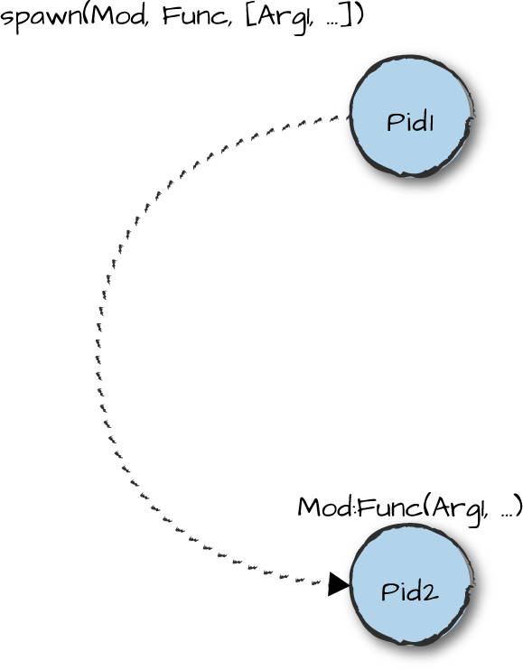
Figure 2-1. Spawning a process

The following example of an “echo” process shows these basics. The first action of the go/0 function is to spawn a process executing loop/0, after which it communicates with that process by sending and receiving messages. The loop/0 function receives messages and, depending on their format, either replies to them (and loops) or terminates. To get this looping behavior, the function is tail recursive, ensuring it executes in constant memory space.

We know the pid of the process executing loop/0 from the spawn, but when we send it a message, how can it communicate back to us? We’ll have to send it our pid, which we find using the self() BIF:

-module(echo).
-export([go/0, loop/0]).

go() ->
    Pid = spawn(echo, loop, []),
    Pid ! {self(), hello},
    receive
        {Pid, Msg} ->
        io:format("~w~n",[Msg])
    end,
    Pid ! stop.

loop() ->
    receive
        {From, Msg} ->
            From ! {self(), Msg},
            loop();
        stop ->
            ok
    end.

In this echo example, the go/0 function first spawns a new process executing the echo:loop/0 function, storing the resulting pid in the variable Pid. It then sends to the Pid process a message containing the pid of the sender, retrieved using the self() BIF, along with the atom hello. After that, go/0 waits to receive a message in the form of a pair whose first element matches the pid of the loop process; when such a message arrives, go/0 prints out the second element of the message, exits the receive expression, and finishes by sending the message stop to Pid.

The echo:loop/0 function first waits for a message. If it receives a pair containing a pid From and a message, it sends a message containing its own pid along with the received Msg back to the From process and then calls itself recursively. If it instead receives the atom stop, loop/0 returns ok. When loop/0 stops, the process that go/0 originally spawned to run loop/0 terminates as well, as there is no more code to execute.

Note how, when we run this program, the go/0 call returns stop. Every function returns a value, that of the last expression it evaluated. Here, the last expression is Pid ! go, which returns the message we just sent to Pid:

1> c(echo).
{ok,echo}
2> echo:go().
hello
stop

Erlang message passing is asynchronous: the expression that sends a message to a process returns immediately and always appears to be successful, even when the receiving process doesn’t exist. If the process exists, the messages are placed in the mailbox of the receiving process in the same order in which they are received. They are processed using the receive expression, which pattern matches on the messages in sequential order. Message reception is selective, meaning that messages are not necessarily processed in the order in which they arrive, but rather the order in which they are matched. Each receive clause selects the message it wants to read from the mailbox using pattern matching.

Suppose that the mailbox for the loop process has received the messages foo, stop, and {Pid, hello} in that order. The receive expression will try to match the first message (here, foo) against each of the patterns in turn; this fails, leaving the message in the mailbox. It then tries to do the same with the second message, stop; this doesn’t match the first pattern but does match the second, with the result that the process terminates, as there is no more code to execute.

These semantics mean that we can process messages in whatever order we choose, irrespective of when they arrive. Code like this:

receive
    message1 -> ...
end
receive
    message2 -> ...
end

will process the atoms message1 and then message2. Without this feature, we’d have to anticipate all the different orders in which messages can arrive, and handle each of those, greatly increasing the complexity of our programs. With selective receive, all we do is leave them in the mailbox for later retrieval.

Fail Safe!

In “Recursion and Pattern Matching” we saw the factorial example, and how passing a negative number to the function causes it to raise an exception. This also happens when factorial is applied to something that isn’t a number, in this case the atom zero:

1> ex1:factorial(zero).
** exception error: bad argument in an arithmetic expression
in function  ex1:factorial/1

The alternative to this would be to program defensively, and explicitly identify the case of negative numbers, as well as arguments of any other type, by means of a catch-all clause:

factorial(0) ->
    1;
factorial(N) when N > 0, is_integer(N) ->
    N * factorial(N-1);
factorial(_) ->
    {error,bad_argument}.

The effect of this is would be to require every caller of the function to deal not only with proper results (like 120 = factorial(5)) but also improper ones of the format {error,bad_argument}. If we do this, clients of any function need to understand its failure modes and provide ways of dealing with them, mixing correct computation and error-handling code. How do you handle errors or corrupt data when you do not know what these errors are or how the data got corrupted?

The Erlang design philosophy says “let it fail!” so that a function, process, or other running entity deals only with the correct case and leaves it to other parts of the system (specifically designed to do this) to deal with failure. One way of dealing with failure in sequential code is to use the mechanism for exception handling given by the try-catch construct. Using the definition:

factorial(0) ->
    1;
factorial(N) when N > 0, is_integer(N) ->
    N * factorial(N-1).

we can see the construct in action:

2> ex1:factorial(zero).
** exception error: no function clause matching ex1:factorial(zero)
3> try ex1:factorial(zero) catch Type:Error -> {Type, Error} end.
{error,function_clause}
4> try ex1:factorial(-2) catch Type:Error -> {Type, Error} end.
{error,function_clause}
5> try ex1:factorial(-2) catch error:Error2 -> {error, Error2} end.
{error,function_clause}
6> try ex1:factorial(-2) catch error:Error3 -> {error, Error3};
6>                             exit:Reason  -> {exit, Reason} end.
{error,function_clause}

The try-catch construct gives the user the opportunity to match on the different kinds of exceptions in the clauses, handling them individually. In this example, we match on an error exception caused by a pattern match failure. There are also exit and throw exceptions, the first being the result of a process calling the exit BIF and the latter the result of a user-generated exception using the throw expression.

Links and Monitors for Supervision

A typical Erlang system has lots of (possibly dependent) processes running at the same time. How do these dependencies work with the “let it fail” philosophy? Suppose process A interacts with processes B and C (Figure 2-2); these processes are dependent on each other, so if A fails, they can no longer function properly. A’s failure needs to be detected, after which B and C need to be terminated before restarting them all. In this section we describe the mechanisms that support this approach, namely process linking, exit signals, and monitoring. These simple constructs enable us to build libraries with complex supervision strategies, allowing us to manage processes that may be subjected to failure at any time.

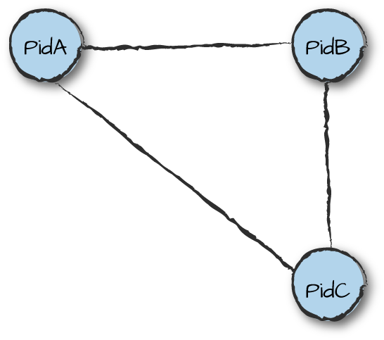
Figure 2-2. Dependent processes

Links

Calling link(Pid) in a process A creates a bidirectional link between processes A and Pid. Calling spawn_link/3 has the same effect as calling spawn/3 followed by link/1, except that it is executed atomically, eliminating the race condition where a process terminates between the spawn and the link. A link from the calling process to Pid is removed by calling unlink(Pid).

The key insight here is that the mechanism needs to be orthogonal to Erlang message passing, but effectuated with it. If two Erlang processes are linked, when either of them terminates, an exit signal is sent to the other, which will then itself terminate. The terminated process will in turn send the exit signal to all the processes in its linked set, propagating it through the system. This can be seen in Figure 2-3, where PidC terminates from whichever exit signal from PidA or PidB gets there first. The power of the mechanism comes from the ways that this default behavior can be modified, giving the designer fine control over the termination of the processes within a system. We now look at this in more detail.

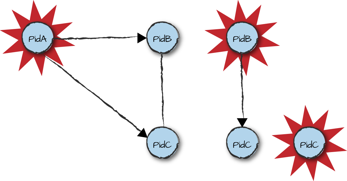
Figure 2-3. Exit signals propagating among linked processes

One pattern for using links is as follows: a server that controls access to resources links to a client while that client has access to a particular resource. If the client terminates, the server will be informed so it can reallocate the resource (or just terminate). If, on the other hand, the client hands back the resource, the server may unlink from the client.

Remember, though, that links are bidirectional, so if the server dies for some reason while client and server are linked, this will by default kill the client too, which you may not want to happen. If that’s the case, use a monitor instead of a link, as we explain in “Monitors”.

Exit signals can be trapped by calling the process_flag(trap_exit, true) function. This converts exit signals into messages of the form {'EXIT', Pid, Reason}, where Pid is the process identifier of the process that has died and Reason is the reason it has terminated. These messages are stored in the recipient’s mailbox and processed in the same way as all other messages. When a process is trapping exits, the exit signal is not propagated to any of the processes in its link set.

Why does a process exit? This can happen for two reasons. If a process has no more code to execute, it terminates normally. The Reason propagated will be the atom normal. Abnormal termination is initiated in case of a runtime error, receiving an exit signal when not trapping exits, or by calling the exit BIFs. Called with a single argument, exit(Reason) will terminate the calling process with reason Reason, which will be propagated in the exit signal to any other processes to which the exiting one is linked. When the exit BIF is called with two arguments, exit(Pid, Reason), it sends an exit signal with reason Reason to the process Pid. This will have the same effect as if the calling process had terminated with reason Reason.

As we said at the start of this section, users can control the way in which termination is propagated through a system. The options are summarized in Table 2-1 and vary depending on if the trap_exit process flag is set.

Table 2-1. Propagation semantics

Reason	Trapping exits	Not trapping exits
normal	Receives {'EXIT', Pid, normal}	Nothing happens
kill	Terminates with reason killed	Terminates with reason killed
Other	Receives {'EXIT', Pid, Other}	Terminates with reason Other

As the second column of the table shows, a process that is trapping exits will receive an 'EXIT' message when a linked process terminates, whether the termination is normal or abnormal. The kill reason allows one process to force another to exit along with it. This means that there’s a mechanism for killing any process, even those that trap exits; note that its reason for termination is killed and not kill, ensuring that the unconditional termination does not itself propagate. If a process is not trapping exits, nothing happens if a process in its link set terminates normally. Abnormal termination, however, results in the process terminating.

1> Pid = spawn(echo, loop, []).
<0.34.0>
2> erlang:monitor(process, Pid).
#Ref<0.0.0.34>
3> exit(Pid, kill).
true
4> flush().
Shell got {'DOWN',#Ref<0.0.0.34>,process,<0.34.0>,killed}
ok

Records

Erlang tuples provide a way of grouping related items, and unlike lists they provide convenient access to elements at arbitrary indexes via the element/2 BIF. In practice, though, they are most useful and manageable for groups of no more than about five or six items. Tuples larger than that can cause maintenance headaches by forcing you to keep track throughout your code of what field is in which position in the tuple, and using plain numbers to address fields through element/2 is error-prone. Pattern matching large tuples can be tedious due to having to ensure the correct number and placement of variables within the tuple. Worst of all, though, is that if you have to add or remove a field in a tuple, you have to find all the places your code uses it and make sure to change each occurrence to the correct new size.

Records address the shortcomings of tuples by providing a way to access fields of a tuple-like collection by name. Here’s an example of a record used with the Erlang/OTP inet module, which provides access to TCP/IP information:

-record(hostent,
        {
         h_name            % offical name of host
         h_aliases = []    % alias list
         h_addrtype        % host address type
         h_length          % length of address
         h_addr_list = []  % list of addresses from name server
        }).

The -record directive is used to define a record, with the record name specified as the directive’s first argument. The second argument, which resembles a tuple of atoms, defines the fields of the record. Fields can have specific default values, as shown here for the h_aliases and h_addr_list fields, both of which have the empty list as their defaults. Fields without specified defaults have the atom undefined as their default values.

Records can be used in assignments, in pattern matching, and as function arguments, similarly to tuples. But unlike tuples, record fields are accessed by name, and any fields not pertinent to a particular part of the code can be left out. For example, the type/1 function in this module requires access only to the h_addrtype field of a hostent record:

-module(addr).
-export([type/1]).

-include_lib("kernel/include/inet.hrl").

type(Addr) ->
    {ok, HostEnt} = inet:gethostbyaddr(Addr),
    HostEnt#hostent.h_addrtype.

First, note that to be able to use a record, we must have access to its definition. The -include_lib(...) directive here includes the inet.hrl file from the kernel application, where the hostent record is defined. In the final line of this example, we access the HostEnt variable as a hostent record by supplying the record name after the # symbol. After the record name, we access the required record field by name, h_addrtype. This reads the value stored in that field and returns it as the return value of the type/1 function:

1> c(addr).
{ok,addr}
2> addr:type("127.0.0.1").
inet
3> addr:type("::1").
inet6

Another way to implement the type() function would be to pattern match the h_addrtype field against the return value of the inet:gethostbyaddr/1 function:

type(Addr) ->
    {ok, #hostent{h_addrtype=AddrType}} = inet:gethostbyaddr(Addr),
    AddrType.

Here, the AddrType variable within the pattern match captures the value of the h_addrtype field as part of the match. This form of pattern matching is quite common with records, and is especially useful within function heads to extract fields of interest into local variables. As you can see, this approach is also cleaner than the field access syntax used in the previous example.

To create a record instance, you set the fields as required:

hostent(Host, inet) ->
    #hostent{h_name=Host, h_addrtype=inet, h_length=4,
             h_addr_list=inet:getaddrs(Host, inet)}.

In this example, the hostent/2 function returns a hostent record instance with specific fields set. Any fields not explicitly set in the code retain their default values specified in the record definition.

Records are just syntactic sugar; under the covers, they are implemented as tuples. We can see this by calling the inet:gethostbyname/1 function in the Erlang shell:

1> inet:gethostbyname("oreilly.com").
{ok,{hostent,"oreilly.com",[],inet,4,
             [{208,201,239,101},{208,201,239,100}]}}
2> rr(inet).
[connect_opts,hostent,listen_opts,...]
3> inet:gethostbyname("oreilly.com").
{ok,#hostent{h_name = "oreilly.com",h_aliases = [],
             h_addrtype = inet,h_length = 4,
             h_addr_list = [{208,201,239,101},{208,201,239,100}]}}

In shell command 1, we call gethostbyname/1 to retrieve address information for the host oreilly.com. The second element of the result tuple is a hostent record, but the shell displays it as a plain tuple where the first element is the record name and the rest of the elements are the fields of the record in declaration order. Note that the names of the record fields are not part of the actual record instance. To have the record instance be displayed as a record instead of a tuple, we need to inform the shell of the record definition. We do that in shell command 2 using the rr shell command, which reads record definitions from its argument and returns a list of the definitions read (we abbreviated the returned list in this example by replacing most of it with an ellipsis). The argument passed to the rr command can either be a module name, the name of a source or include file, or a wildcarded name as specified for the filelib:wildcard/1,2 functions. In shell command 3, we again fetch address information for oreilly.com, but this time the shell prints the returned hostent value in record format, with field names included.

Maps

A map in Erlang is a key-value collection type that resembles the dictionary and hash types found in other programming languages. Maps differ from records in several ways: map is a built-in type, the number of its fields or key-value pairs is not fixed at compile time, and its keys can be any Erlang term rather than just atoms. While some have touted maps as a replacement for records, in practice they each fulfill different needs and both are useful. Records are fast, so use them when you have a fixed number of fields known at compile time, while maps should be used when you have a need to add fields at runtime.

Creating and manipulating a map is straightforward, as shown here:

1> EmptyMap = #{}.
#{}
2> erlang:map_size(EmptyMap).
0
3> RelDates = #{ "R15B03-1" => {2012, 11, 28}, "R16B03" => {2013, 12, 11} }.
#{"R15B03-1" => {2012,11,28},"R16B03" => {2013,12,11}}
4> RelDates2 = RelDates#{ "17.0" => {2014, 4, 2}}.
#{"17.0" => {2014,4,2},
  "R15B03-1" => {2012,11,28},
  "R16B03" => {2013,12,11}}
5> RelDates3 = RelDates2#{"17.0" := {2014, 4, 9}}.
#{"17.0" => {2014,4,9},
  "R15B03-1" => {2012,11,28},
  "R16B03" => {2013,12,11}}
6> #{ "R15B03-1" := Date } = RelDates3.
#{"17.0" => {2014,4,2},
  "R15B03-1" => {2012,11,28},
  "R16B03" => {2013,12,11}}
7> Date.
{2012,11,28}

In shell command 1, we bind the empty map #{} to the variable EmptyMap, and then we check its size in shell command 2 using the erlang:map_size/1 function. As expected, its size is 0 since it contains no key-value pairs. In shell command 3, we create a map with multiple entries, where each key is the name of an Erlang/OTP release paired with a value denoting its release date, using the => map association operator. Shell command 4 takes the existing RelDates map and adds a new key-value pair to create a new map, RelDates2. Unfortunately, the date we set in shell command 4 is off by one week and we need to change it; shell command 5 shows how we use the := map set-value operator to update the release date. Unlike the => operator, the := operator ensures that the key being updated already exists in the map, thereby preventing errors where the developer misspells the key and accidentally creates a new key-value pair instead of updating an existing key. Finally, shell command 6 shows how using a map in a pattern match allows us to capture the release date associated with the key "R15B03-1" into the variable Date, the value of which is accessed in shell command 7. Note that using the := set-value operator is required for map pattern matching.

Macros

Erlang has a macro facility, implemented by the Erlang preprocessor (epp), which is invoked prior to compilation of source code into BEAM code. Macros can be constants, as in:

-define(ANSWER,42).
-define(DOUBLE,2*).

or take parameters, as in:

-define(TWICE(F,X),F(F(X))).

As you can see from the definition of DOUBLE, it is conventional (but only conventional) to use uppercase names. The definition can be any legal sequence of Erlang tokens; it doesn’t have to be a meaningful expression in its own right.

Macros are invoked by preceding them with a ? character, as in:

test() -> ?TWICE(?DOUBLE,?ANSWER)

It is possible to see the effect of macro definitions by compiling with the 'P' flag in the shell:

c(<filename>,['P']),

which creates a filename.P file in which the previous definition of test/0 becomes:

test() -> 2 * (2 * 42).

It is also possible for a macro call to record the text of its parameters. For example, if we define:

 -define(Assign(Var,Exp), Var=Exp,
         io:format("~s = ~s -> ~p~n",[??Var,??Exp,Var]) ).

then ?Assign(Var,Exp) has the effect of performing the assignment Var = Exp, but also, as a side effect, prints out a diagnostic message. For example:

test_assign() -> ?Assign(X, lists:sum([1,2,3])).

behaves like this:

1> macros:test_assign().
X = lists : sum ( [ 1 , 2 , 3 ] ) -> 6
ok

Using flags, you can define conditional macros, such as:

-ifdef(debug).
  -define(Assign(Var,Exp), Var=Exp,
          io:format("~s = ~s -> ~p~n",[??Var,??Exp,Var]) ).
-else.
  -define(Assign(Var,Exp), Var=Exp).
-endif.

Now, if you use the compiler flags {d,debug} to set the debug flag, ?Assign(Var,Exp) will perform the assignment and print out the diagnostic code. Conversely, leaving the debug flag unset by default or clearing it through {u,debug} will cause the program to do the assignment without executing the io expression.

Upgrading Modules

One of the advantages of dynamic typing is the ability to upgrade your code during runtime, without the need to take down the system. One second, you are running a buggy version of a module, but you can load a fix without terminating the process and it starts running the fixed version, retaining its state and variables (Figure 2-4). This works not only for bugs, but also for upgrades and new features. This is a crucial property for a system that needs to guarantee “five-nines availability”—i.e., 99.999% uptime including upgrades and maintenance.

Figure 2-4. A software upgrade

At any one time, two versions of a module may exist in the virtual machine: the old and current versions. Frame 1 in Figure 2-4 shows PidA executing in the current version of module B. In Frame 2, new code for the module B is loaded, either by compiling the module in the shell or by explicitly loading it. After you load the module, PidA is still linked to the same version of B, which has now become the old version. But the next time PidA makes a fully qualified call to a function in module B, a check will be made to ensure that PidA is running the latest version of the code. (If you recall from earlier in this chapter, a fully qualified call is one where the module name is prefixed to the function name.) If the process is not running the latest version, the pointer to the code will be switched to the new current version, as shown in Frame 3. This applies to all functions in B, not just the function whose call triggered the switch. While this is the essence of a software upgrade, let’s go through the fine print to make sure you understand all the details:

• Suppose that the code for the loop of a running process is itself upgraded. The effect depends on the form of the function call. If the function call is fully qualified—i.e., of the form B:loop()—the next call will use the upgraded code; otherwise (when the call is simply loop()), the process will continue to run the old code.

• The system holds only two versions of the code, so suppose that process p is still executing v(1) of module B, and another two new versions v(2) and v(3) are loaded: since only two versions may be present, the earliest version v(1) will be purged, and any process (such as p) looping in that version of the module will be unconditionally terminated.

• New code can be loaded in a number of ways. Compiling the module will cause code to be reloaded; this can be initiated in the shell by c(Module) or by calling the Erlang function compile:file(Module). Code can also be loaded explicitly in the shell by l(Module) or by a call to code:load_file(Module). In general, code is loaded by calling a function in a module that is not already loaded. This causes the compiled code, a .beam file, to be loaded, and for that to happen the code has to have been already compiled, perhaps using the erlc command-line tool. Note that recompiling a module with erlc does not cause it to be reloaded.

• While old code is purged when a new version is loaded, it is possible to call code:purge(Module) explicitly to purge an old version (without loading a new version). This has the effect of terminating all processes running the old code before removing the code. The call returns true if any processes were indeed terminated, and false if none were. Calling code:soft_purge(Module) will remove the code only if no processes were running it: the result is true in that case and false otherwise.

ETS: Erlang Term Storage

While lists are an important data type, they need to be linearly traversed and, as a result, will not scale. If you need a key-value store where the lookup time is constant, or the ability to traverse your keys in lexicographical order, Erlang Term Storage (ETS) tables come in handy. An ETS table is a collection of Erlang tuples, keyed on a particular position in the tuple.

ETS tables come in four different kinds:

Set

Each key-value tuple can occur only once.

Bag

Each key-value tuple combination can only occur once, but a key can appear multiple times.

Duplicate bag

Tuples can be duplicated.

Ordered set

These have the same restriction as sets, but the tuples can be visited in order by key.

Access time to a particular element is in constant time, except for ordered sets, where access time is proportional to the logarithm of the size of the table (O(log n) time).

Depending on the options passed in at table creation (ets:new), tables have one of the following traits:

public

Accessible to all processes.

private

Accessible to the owning process only.

protected

All processes can read the table, but only the owner can write to it.

Tables can also have their key position specified at creation time ({keypos,N}). This is mainly useful when storing records, as it allows the developer to specify a particular field of the record as the key. The default key position is 1.

Normally, programs access tables through the table ID returned by the call to new, but tables can also be named when created, which makes them accessible by name.

A table is linked to the process that creates it, and is deleted when that process terminates. ETS tables are in-memory only, but long-lived tables are provided by DETS tables, which are stored on disk (hence the “D”).

Elementary table operations are shown in the following interaction:

1> TabId = ets:new(tab,[named_table]).
tab
2> ets:insert(tab,{haskell, lazy}).
true
3> ets:lookup(tab,haskell).
[{haskell,lazy}]
4> ets:insert(tab,{haskell, ghci}).
true
5> ets:lookup(tab,haskell).
[{haskell,ghci}]
6> ets:lookup(tab,racket).
[]

As can be seen, the default ETS table is a set, so that the insertion at line 4 overwrites the insertion at line 2, and the table is keyed at the first position. Note also that looking up a key returns a list of all the tuples matching the key.

Tables can be traversed, as seen here:

7> ets:insert(tab,{racket,strict}).
true
8> ets:insert(tab,{ocaml,strict}).
true
9> ets:first(tab).
racket
10> ets:next(tab,racket).
haskell

Since tab is a set ETS, the elements are not ordered by key; instead, their ordering is determined by a hash value internal to the table implementation. In the example here, the first key is racket and the next is haskell. However, using first and next on an ordered set will give traversal in order by key. It is also possible to extract bulk information using the match function:

11> ets:match(tab,{'$1','$0'}).
[[strict,ocaml],[ghci,haskell],[strict,racket]]
12> ets:match(tab,{'$1','_'}).
[[ocaml],[haskell],[racket]]
13> ets:match(tab,{'$1',strict}).
[[ocaml],[racket]]

The second argument, which is a symbolic tuple, is matched against the tuples in the ETS table. The result is a list of lists, with each list giving the values matched to the named variables '$0' etc., in ascending order; these variables match any value in the tuple. The wildcard value '_' also matches any value, but its argument is not reported in the result.

Let’s implement code that uses an ETS table to associate phone numbers—or more accurately, mobile subscriber integrated services digital network (MSISDN) numbers—to pids in a module called hlr. We create the associations when phones attach themselves to the network and delete them when they detach. We then allow users to look up the pid associated with a particular phone number as well as the number associated with a pid. Read through this code, as we use it as part of a larger example in later chapters:

-module(hlr).
-export([new/0, attach/1, detach/0, lookup_id/1, lookup_ms/1]).

new() ->
    ets:new(msisdn2pid, [public, named_table]),
    ets:new(pid2msisdn, [public, named_table]),
    ok.

attach(Ms) ->
    ets:insert(msisdn2pid, {Ms, self()}),
    ets:insert(pid2msisdn, {self(), Ms}).

detach() ->
    case ets:lookup(pid2msisdn, self()) of
        [{Pid, Ms}] ->
            ets:delete(pid2msisdn, Pid),
            ets:delete(msisdn2pid, Ms);
        [] ->
            ok
    end.

lookup_id(Ms) ->
    case ets:lookup(msisdn2pid, Ms) of
        [] -> {error, invalid};
        [{Ms, Pid}] -> {ok, Pid}
    end.

lookup_ms(Pid) ->
    case ets:lookup(pid2msisdn, Pid) of
        [] -> {error, invalid};
        [{Pid, Ms}] -> {ok, Ms}
    end.

In our test run of the module, the shell process attaches itself to the network using the number 12345. We look up the mobile handset using both the number and the pid, after which we detach. When reading the code, note that we are using a named public table, meaning any process can read and write to it as long as they know the table name:

2> hlr:new().
ok
3> hlr:attach(12345).
true
4> hlr:lookup_ms(self()).
{ok,12345}
5> hlr:lookup_id(12345).
{ok,<0.32.0>}
6> hlr:detach().
true
7> hlr:lookup_id(12345).
{error,invalid}

Distributed Erlang

All of the examples we have looked at so far execute on a single virtual machine, also referred to as a node. Erlang has built-in semantics allowing programs to run across multiple nodes: processes can transparently spawn processes on other nodes and communicate with them using message passing. Distributed nodes can reside either on the same physical or virtual host or on different ones.

This programming model is designed to support scaling and fault tolerance on systems running behind firewalls over trusted networks. Out of the box, Erlang distribution is not designed to support systems operating across potentially hostile environments such as the Internet or shared cloud instances. Because different systems have different requirements on security, no one size fits all. Varying security requirements can easily (or not so easily) be addressed if you provide your own security layers and authentication mechanisms, or by modifying Erlang’s networking and security libraries.

monitor_node(Node, true),
{serve, Node} ! {self(), Msg},
receive
    {ok, Resp} ->
        monitor_node(Node, false),
        <handle process response>;  % Pseudocode to handle the process response
    {nodedown, Node} ->
        <handle lack of response>   % Pseudocode to handle lack of response
end.

 erl -sname foo -setcookie abc
 erl -sname bar -setcookie abc

$ erl -sname bar -setcookie abc
Erlang/OTP 18 [erts-7.2] [smp:8:8] [async-threads:10] [kernel-poll:false]

Eshell V7.2  (abort with ^G)
(bar@macbook-pro-2)1> net_adm:ping('foo@macbook-pro-2').
pong
(bar@macbook-pro-2)2> [Node] = nodes().
['foo@macbook-pro-2']
(bar@macbook-pro-2)3> Shell = self(). 
<0.38.0>
(bar@macbook-pro-2)4> spawn(Node, fun() -> Shell ! self() end).
<5985.46.0>
(bar@macbook-pro-2)5> receive Pid -> Pid end.
<5985.46.0>
(bar@macbook-pro-2)6> node(Pid).
'foo@macbook-pro-2'
(bar@macbook-pro-2)7> spawn(Node, fun() -> Shell ! node() end).
<5985.47.0>
(bar@macbook-pro-2)8> flush().
Shell got 'foo@macbook-pro-2'
ok

Summing Up

In this chapter, we’ve given an overview of the basics of Erlang we believe are important for understanding the examples in the remainder of the book. The concurrency model, error-handling semantics, and distributed processing not only make Erlang a powerful tool, but are the foundation of OTP’s design. Module upgrades during runtime is just the icing on the cake. Before you progress, be warned that the better you understand the internals of Erlang, the more you are going to get out of the OTP design principles and this book. We provide many more examples written in pure Erlang, which for some might be enough to understand the OTP rationale. Try moving ahead, but if you find yourself struggling, we suggest reading Erlang Programming, published by O’Reilly and coauthored by one of the authors of this book. The current book can be seen as a continuation of Erlang Programming, expanding many of the original examples from that book. Other great titles that will also do the trick include Simon St. Laurent’s Introducing Erlang, also published by O’Reilly; Fred Hébert’s Learn You Some Erlang for Great Good! from No Starch Press (and also available online free of charge); and Programming Erlang, written by Erlang coinventor Joe Armstrong and published by The Pragmatic Bookshelf.

What’s Next?

In the upcoming chapters, we introduce process design patterns and OTP behaviors. We start by providing an Erlang example of a client-server application, breaking it up into generic and specific parts. The generic parts are those that can be reused from one client-server application to another and are packaged in library modules. The specific parts are those that are project-specific and have to be implemented for the individual client-server applications. In Chapter 4, we migrate the code to an OTP-based generic server behavior, introducing the first building block of Erlang-based systems. As more behaviors are introduced in the subsequent chapters, it will become clear how Erlang systems are architected and glued together.