
CHAPTER
5
Information Theory
5.1 Introduction
As mentioned in Chapter 1 and reiterated along the way, the purpose of a communication system is to facilitate the transmission of signals generated by a source of information over a communication channel. But, in basic terms, what do we mean by the term information? To address this important issue, we need to understand the fundamentals of information theory.1
The rationale for studying the fundamentals of information theory at this early stage in the book is threefold:
1. Information theory makes extensive use of probability theory, which we studied in Chapter 3; it is, therefore, a logical follow-up to that chapter.
2. It adds meaning to the term “information” used in previous chapters of the book.
3. Most importantly, information theory paves the way for many important concepts and topics discussed in subsequent chapters.
In the context of communications, information theory deals with mathematical modeling and analysis of a communication system rather than with physical sources and physical channels. In particular, it provides answers to two fundamental questions (among others):
1. What is the irreducible complexity, below which a signal cannot be compressed?
2. What is the ultimate transmission rate for reliable communication over a noisy channel?
The answers to these two questions lie in the entropy of a source and the capacity of a channel, respectively:
1. Entropy is defined in terms of the probabilistic behavior of a source of information; it is so named in deference to the parallel use of this concept in thermodynamics.
2. Capacity is defined as the intrinsic ability of a channel to convey information; it is naturally related to the noise characteristics of the channel.
A remarkable result that emerges from information theory is that if the entropy of the source is less than the capacity of the channel, then, ideally, error-free communication over the channel can be achieved. It is, therefore, fitting that we begin our study of information theory by discussing the relationships among uncertainty, information, and entropy.
5.2 Entropy
Suppose that a probabilistic experiment involves observation of the output emitted by a discrete source during every signaling interval. The source output is modeled as a stochastic process, a sample of which is denoted by the discrete random variable S. This random variable takes on symbols from the fixed finite alphabet
![]()
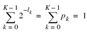
Of course, this set of probabilities must satisfy the normalization property

We assume that the symbols emitted by the source during successive signaling intervals are statistically independent. Given such a scenario, can we find a measure of how much information is produced by such a source? To answer this question, we recognize that the idea of information is closely related to that of uncertainty or surprise, as described next.
Consider the event S = sk, describing the emission of symbol sk by the source with probability pk, as defined in (5.2). Clearly, if the probability pk = 1 and pi = 0 for all i ≠ k, then there is no “surprise” and, therefore, no “information” when symbol sk is emitted, because we know what the message from the source must be. If, on the other hand, the source symbols occur with different probabilities and the probability pk is low, then there is more surprise and, therefore, information when symbol sk is emitted by the source than when another symbol si, i ≠ k, with higher probability is emitted. Thus, the words uncertainty, surprise, and information are all related. Before the event S = sk occurs, there is an amount of uncertainty. When the event S = sk occurs, there is an amount of surprise. After the occurrence of the event S = sk, there is gain in the amount of information, the essence of which may be viewed as the resolution of uncertainty. Most importantly, the amount of information is related to the inverse of the probability of occurrence of the event S = sk.
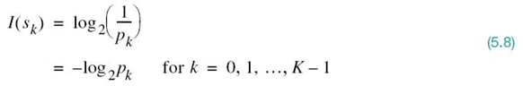
We define the amount of information gained after observing the event S = sk, which occurs with probability pk, as the logarithmic function2

which is often termed “self-information” of the event S = sk. This definition exhibits the following important properties that are intuitively satisfying:
PROPERTY 1
![]()
Obviously, if we are absolutely certain of the outcome of an event, even before it occurs, there is no information gained.
PROPERTY 2
![]()
That is to say, the occurrence of an event S = sk either provides some or no information, but never brings about a loss of information.
PROPERTY 3
![]()
That is, the less probable an event is, the more information we gain when it occurs.
PROPERTY 4
I(sk, sl) = I(sk) + I(sl) if sk and sl are statistically independent
This additive property follows from the logarithmic definition described in (5.4).
The base of the logarithm in (5.4) specifies the units of information measure. Nevertheless, it is standard practice in information theory to use a logarithm to base 2 with binary signaling in mind. The resulting unit of information is called the bit, which is a contraction of the words binary digit. We thus write
When pk = 1/2, we have I(sk) = 1 bit. We may, therefore, state:
One bit is the amount of information that we gain when one of two possible and equally likely (i.e., equiprobable) events occurs.
Note that the information I(sk) is positive, because the logarithm of a number less than one, such as a probability, is negative. Note also that if pk is zero, then the self-information Isk assumes an unbounded value.
The amount of information I(sk) produced by the source during an arbitrary signaling interval depends on the symbol sk emitted by the source at the time. The self-information I(sk) is a discrete random variable that takes on the values I(s0), I(s1),…,I(sK – 1) with probabilities p0, p1,…,pK – 1 respectively. The expectation of I(sk) over all the probable values taken by the random variable S is given by
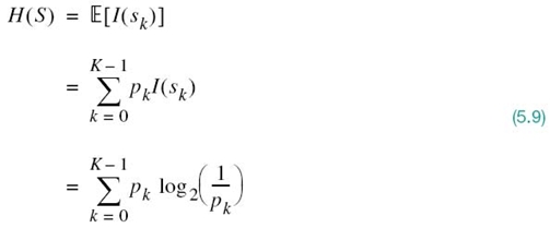
The quantity H(S) is called the entropy,3 formally defined as follows:
The entropy of a discrete random variable, representing the output of a source of information, is a measure of the average information content per source symbol.
Note that the entropy H(S) is independent of the alphabet ![]() ; it depends only on the probabilities of the symbols in the alphabet
; it depends only on the probabilities of the symbols in the alphabet ![]() of the source.
of the source.
Properties of Entropy
Building on the definition of entropy given in (5.9), we find that entropy of the discrete random variable S is bounded as follows:
where K is the number of symbols in the alphabet ![]() .
.
Elaborating on the two bounds on entropy in (5.10), we now make two statements:
1. H(S) = 0, if, and only if, the probability pk = 1 for some k, and the remaining probabilities in the set are all zero; this lower bound on entropy corresponds to no uncertainty.
2. H(S) = log K, if, and only if, pk = 1/K for all k (i.e., all the symbols in the source alphabet ![]() are equiprobable); this upper bound on entropy corresponds to maximum uncertainty.
are equiprobable); this upper bound on entropy corresponds to maximum uncertainty.
To prove these properties of H(S), we proceed as follows. First, since each probability pk is less than or equal to unity, it follows that each term pklog2(1/pk) in (5.9) is always nonnegative, so H(S) ≥ 0. Next, we note that the product term pk log2(1/pk) is zero if, and only if, pk = 0 or 1. We therefore deduce that H(S) = 0 if, and only if, pk = 0 or 1 for some k and all the rest are zero. This completes the proofs of the lower bound in (5.10) and statement 1.
To prove the upper bound in (5.10) and statement 2, we make use of a property of the natural logarithm:
where loge is another way of describing the natural logarithm, commonly denoted by ln; both notations are used interchangeably. This inequality can be readily verified by plotting the functions lnx and (x – 1) versus x, as shown in Figure 5.1. Here we see that the line y = x – 1 always lies above the curve y = logex. The equality holds only at the point x = 1, where the line is tangential to the curve.
To proceed with the proof, consider first any two different probability distributions denoted by p0, p1,…,pK – 1 and q0, q1,…,qK – 1 on the alphabet ![]() = {s0, s1,…,sK – 1) of a discrete source. We may then define the relative entropy of these two distributions:
= {s0, s1,…,sK – 1) of a discrete source. We may then define the relative entropy of these two distributions:
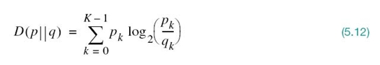
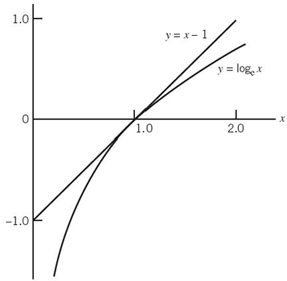
Figure 5.1 Graphs of the functions x – 1 and log x versus x.
Hence, changing to the natural logarithm and using the inequality of (5.11), we may express the summation on the right-hand side of (5.12) as follows:
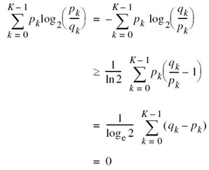
where, in the third line of the equation, it is noted that the sums over pk and qk are both equal to unity in accordance with (5.3). We thus have the fundamental property of probability theory:
![]()
In words, (5.13) states:
The relative entropy of a pair of different discrete distributions is always nonnegative; it is zero only when the two distributions are identical.
Suppose we next put
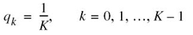
which corresponds to a source alphabet ![]() with equiprobable symbols. Using this distribution in (5.12) yields
with equiprobable symbols. Using this distribution in (5.12) yields
where we have made use of (5.3) and (5.9). Hence, invoking the fundamental inequality of (5.13), we may finally write
Thus, H(S) is always less than or equal to log2 K. The equality holds if, and only if, the symbols in the alphabet ![]() are equiprobable. This completes the proof of (5.10) and with it the accompanying statements 1 and 2.
are equiprobable. This completes the proof of (5.10) and with it the accompanying statements 1 and 2.
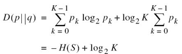
EXAMPLE 1 Entropy of Bernoulli Random Variable
To illustrate the properties of H(S) summed up in (5.10), consider the Bernoulli random variable for which symbol 0 occurs with probability p0 and symbol 1 with probability p1 = 1 – p0.
The entropy of this random variable is
from which we observe the following:
1. When p0 = 0, the entropy H(S) = 0; this follows from the fact that xloge x → 0 as x → 0.
2. When p0 = 1, the entropy H(S) = 0.
3. The entropy H(S) attains its maximum value Hmax = 1 bit when p1 = p0 = 1/2; that is, when symbols 1 and 0 are equally probable.
In other words, H(S) is symmetric about p0 = 1/2.
The function of p0 given on the right-hand side of (5.15) is frequently encountered in information-theoretic problems. It is customary, therefore, to assign a special symbol to this function. Specifically, we define
We refer to H(p0) as the entropy function. The distinction between (5.15) and (5.16) should be carefully noted. The H(S) of (5.15) gives the entropy of the Bernoulli random variable S. The H(p0) of (5.16), on the other hand, is a function of the prior probability p0 defined on the interval [0, 1]. Accordingly, we may plot the entropy function H(p0) versus p0, defined on the interval [0, 1], as shown in Figure 5.2. The curve in Figure 5.2 highlights the observations made under points 1, 2, and 3.

Figure 5.2 Entropy function H(p0).
Extension of a Discrete Memoryless Source
To add specificity to the discrete source of symbols that has been the focus of attention up until now, we now assume it to be memoryless in the sense that the symbol emitted by the source at any time is independent of previous and future emissions.
In this context, we often find it useful to consider blocks rather than individual symbols, with each block consisting of n successive source symbols. We may view each such block as being produced by an extended source with a source alphabet described by the Cartesian product of a set Sn that has Kn distinct blocks, where K is the number of distinct symbols in the source alphabet S of the original source. With the source symbols being statistically independent, it follows that the probability of a source symbol in Sn is equal to the product of the probabilities of the n source symbols in S that constitute a particular source symbol of Sn. We may thus intuitively expect that H(Sn), the entropy of the extended source, is equal to n times H(S), the entropy of the original source. That is, we may write
We illustrate the validity of this relationship by way of an example.
EXAMPLE 2 Entropy of Extended Source
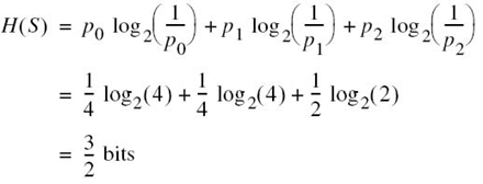
Consider a discrete memoryless source with source alphabet ![]() = {s0, s1, s2}, whose three distinct symbols have the following probabilities:
= {s0, s1, s2}, whose three distinct symbols have the following probabilities:

Hence, the use of (5.9) yields the entropy of the discrete random variable S representing the source as
Consider next the second-order extension of the source. With the source alphabet ![]() consisting of three symbols, it follows that the source alphabet of the extended source S(2) has nine symbols. The first row of Table 5.1 presents the nine symbols of S(2), denoted by σ0, σ1,…,σ8. The second row of the table presents the composition of these nine symbols in terms of the corresponding sequences of source symbols s0, s1, and s2, taken two at a time. The probabilities of the nine source symbols of the extended source are presented in the last row of the table. Accordingly, the use of (5.9) yields the entropy of the extended source as
consisting of three symbols, it follows that the source alphabet of the extended source S(2) has nine symbols. The first row of Table 5.1 presents the nine symbols of S(2), denoted by σ0, σ1,…,σ8. The second row of the table presents the composition of these nine symbols in terms of the corresponding sequences of source symbols s0, s1, and s2, taken two at a time. The probabilities of the nine source symbols of the extended source are presented in the last row of the table. Accordingly, the use of (5.9) yields the entropy of the extended source as
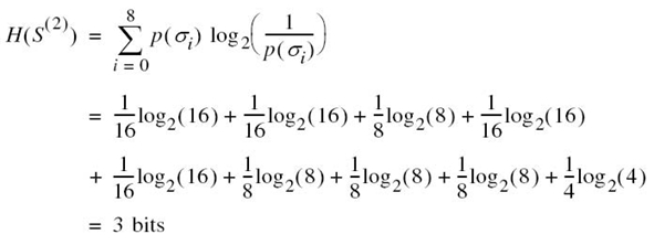
Table 5.1 Alphabets of second-order extension of a discrete memoryless source

We thus see that H(S (2)) = 2H(S) in accordance with (5.17).
5.3 Source-coding Theorem
Now that we understand the meaning of entropy of a random variable, we are equipped to address an important issue in communication theory: the representation of data generated by a discrete source of information.
The process by which this representation is accomplished is called source encoding. The device that performs the representation is called a source encoder. For reasons to be described, it may be desirable to know the statistics of the source. In particular, if some source symbols are known to be more probable than others, then we may exploit this feature in the generation of a source code by assigning short codewords to frequent source symbols, and long codewords to rare source symbols. We refer to such a source code as a variable-length code. The Morse code, used in telegraphy in the past, is an example of a variable-length code. Our primary interest is in the formulation of a source encoder that satisfies two requirements:
1. The codewords produced by the encoder are in binary form.
2. The source code is uniquely decodable, so that the original source sequence can be reconstructed perfectly from the encoded binary sequence.
The second requirement is particularly important: it constitutes the basis for a perfect source code.
Consider then the scheme shown in Figure 5.3 that depicts a discrete memoryless source whose output sk is converted by the source encoder into a sequence of 0s and 1s, denoted by bk. We assume that the source has an alphabet with K different symbols and that the kth symbol sk occurs with probability pk, k = 0, 1,…,K – 1. Let the binary codeword assigned to symbol sk by the encoder have length lk, measured in bits. We define the average codeword length ![]() of the source encoder as
of the source encoder as

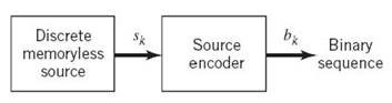
In physical terms, the parameter ![]() represents the average number of bits per source symbol used in the source encoding process. Let Lmin denote the minimum possible value of L. We then define the coding efficiency of the source encoder as
represents the average number of bits per source symbol used in the source encoding process. Let Lmin denote the minimum possible value of L. We then define the coding efficiency of the source encoder as
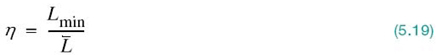
With ![]() ≥ Lmin, we clearly have η ≤ 1. The source encoder is said to be efficient when η approaches unity.
≥ Lmin, we clearly have η ≤ 1. The source encoder is said to be efficient when η approaches unity.
But how is the minimum value Lmin determined? The answer to this fundamental question is embodied in Shannon’s first theorem: the source-coding theorem,4 which may be stated as follows:
Given a discrete memoryless source whose output is denoted by the random variable S, the entropy H(S) imposes the following bound on the average codeword length ![]() for any source encoding scheme:
for any source encoding scheme:
According to this theorem, the entropy H(S) represents a fundamental limit on the average number of bits per source symbol necessary to represent a discrete memoryless source, in that it can be made as small as but no smaller than the entropy H(S). Thus, setting Lmin = H(S), we may rewrite (5.19), defining the efficiency of a source encoder in terms of the entropy H(S) as shown by
where as before we have η ≤ 1.
5.4 Lossless Data Compression Algorithms
A common characteristic of signals generated by physical sources is that, in their natural form, they contain a significant amount of redundant information, the transmission of which is therefore wasteful of primary communication resources. For example, the output of a computer used for business transactions constitutes a redundant sequence in the sense that any two adjacent symbols are typically correlated with each other.
For efficient signal transmission, the redundant information should, therefore, be removed from the signal prior to transmission. This operation, with no loss of information, is ordinarily performed on a signal in digital form, in which case we refer to the operation as lossless data compression. The code resulting from such an operation provides a representation of the source output that is not only efficient in terms of the average number of bits per symbol, but also exact in the sense that the original data can be reconstructed with no loss of information. The entropy of the source establishes the fundamental limit on the removal of redundancy from the data. Basically, lossless data compression is achieved by assigning short descriptions to the most frequent outcomes of the source output and longer descriptions to the less frequent ones.
In this section we discuss some source-coding schemes for lossless data compression. We begin the discussion by describing a type of source code known as a prefix code, which not only is uniquely decodable, but also offers the possibility of realizing an average codeword length that can be made arbitrarily close to the source entropy.
Prefix Coding
Consider a discrete memoryless source of alphabet {s0, s1,…,sK – 1} and respective probabilities {p0, p1,…,pK – 1}. For a source code representing the output of this source to be of practical use, the code has to be uniquely decodable. This restriction ensures that, for each finite sequence of symbols emitted by the source, the corresponding sequence of codewords is different from the sequence of codewords corresponding to any other source sequence. We are specifically interested in a special class of codes satisfying a restriction known as the prefix condition. To define the prefix condition, let the codeword assigned to source symbol sk be denoted by (mk1, mk2,…,mkn), where the individual elements mk1,…,mkn are 0s and 1s and n is the codeword length. The initial part of the codeword is represented by the elements mk1,…,mki for some i ≤ n. Any sequence made up of the initial part of the codeword is called a prefix of the codeword. We thus say:
A prefix code is defined as a code in which no codeword is the prefix of any other codeword.
Prefix codes are distinguished from other uniquely decodable codes by the fact that the end of a codeword is always recognizable. Hence, the decoding of a prefix can be accomplished as soon as the binary sequence representing a source symbol is fully received. For this reason, prefix codes are also referred to as instantaneous codes.
EXAMPLE 3 Illustrative Example of Prefix Coding
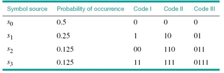
To illustrate the meaning of a prefix code, consider the three source codes described in Table 5.2. Code I is not a prefix code because the bit 0, the codeword for s0, is a prefix of 00, the codeword for s2. Likewise, the bit 1, the codeword for s1, is a prefix of 11, the codeword for s3. Similarly, we may show that code III is not a prefix code but code II is.
Table 5.2 Illustrating the definition of a prefix code
Decoding of Prefix Code
To decode a sequence of codewords generated from a prefix source code, the source decoder simply starts at the beginning of the sequence and decodes one codeword at a time. Specifically, it sets up what is equivalent to a decision tree, which is a graphical portrayal of the codewords in the particular source code. For example, Figure 5.4 depicts the decision tree corresponding to code II in Table 5.2. The tree has an initial state and four terminal states corresponding to source symbols s0, s1, s2, and s3. The decoder always starts at the initial state. The first received bit moves the decoder to the terminal state s0 if it is 0 or else to a second decision point if it is 1. In the latter case, the second bit moves the decoder one step further down the tree, either to terminal state s1 if it is 0 or else to a third decision point if it is 1, and so on. Once each terminal state emits its symbol, the decoder is reset to its initial state. Note also that each bit in the received encoded sequence is examined only once. Consider, for example, the following encoded sequence:
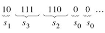
This sequence is readily decoded as the source sequence s1s3s2s0s0…. The reader is invited to carry out this decoding.
As mentioned previously, a prefix code has the important property that it is instantaneously decodable. But the converse is not necessarily true. For example, code III in Table 5.2 does not satisfy the prefix condition, yet it is uniquely decodable because the bit 0 indicates the beginning of each codeword in the code.
To probe more deeply into prefix codes, exemplified by that in Table 5.2, we resort to an inequality, which is considered next.
Kraft Inequality
Consider a discrete memoryless source with source alphabet {s0, s1,…,sK – 1} and source probabilities {p0, p1,…,pK – 1}, with the codeword of symbol sk having length lk, k = 0, 1,…,K – 1. Then, according to the Kraft inequality,5 the codeword lengths always satisfy the following inequality:

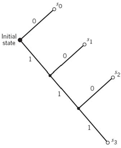
Figure 5.4 Decision tree for code II of Table 5.2.
where the factor 2 refers to the number of symbols in the binary alphabet. The Kraft inequality is a necessary but not sufficient condition for a source code to be a prefix code. In other words, the inequality of (5.22) is merely a condition on the codeword lengths of a prefix code and not on the codewords themselves. For example, referring to the three codes listed in Table 5.2, we see:
- Code I violates the Kraft inequality; it cannot, therefore, be a prefix code.
- The Kraft inequality is satisfied by both codes II and III, but only code II is a prefix code.
Given a discrete memoryless source of entropy H(S), a prefix code can be constructed with an average codeword length ![]() , which is bounded as follows:
, which is bounded as follows:
The left-hand bound of (5.23) is satisfied with equality under the condition that symbol sk is emitted by the source with probability
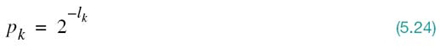
where lk is the length of the codeword assigned to source symbol sk. A distribution governed by (5.24) is said to be a dyadic distribution. For this distribution, we naturally have
Under this condition, the Kraft inequality of (5.22) confirms that we can construct a prefix code, such that the length of the codeword assigned to source symbol sk is –log2 pk. For such a code, the average codeword length is

and the corresponding entropy of the source is
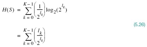
Hence, in this special (rather meretricious) case, we find from (5.25) and (5.26) that the prefix code is matched to the source in that ![]() = H(S).
= H(S).
But how do we match the prefix code to an arbitrary discrete memoryless source? The answer to this basic problem lies in the use of an extended code. Let ![]() denote the average codeword length of the extended prefix code. For a uniquely decodable code,
denote the average codeword length of the extended prefix code. For a uniquely decodable code, ![]() is the smallest possible. From (5.23), we find that
is the smallest possible. From (5.23), we find that
or, equivalently,

In the limit, as n approaches infinity, the lower and upper bounds in (5.28) converge as shown by
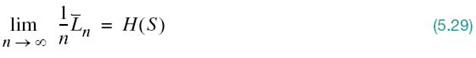
We may, therefore, make the statement:
By making the order n of an extended prefix source encoder large enough, we can make the code faithfully represent the discrete memoryless source S as closely as desired.
In other words, the average codeword length of an extended prefix code can be made as small as the entropy of the source, provided that the extended code has a high enough order in accordance with the source-coding theorem. However, the price we have to pay for decreasing the average codeword length is increased decoding complexity, which is brought about by the high order of the extended prefix code.
Huffman Coding
We next describe an important class of prefix codes known as Huffman codes. The basic idea behind Huffman coding6 is the construction of a simple algorithm that computes an optimal prefix code for a given distribution, optimal in the sense that the code has the shortest expected length. The end result is a source code whose average codeword length approaches the fundamental limit set by the entropy of a discrete memoryless source, namely H(S). The essence of the algorithm used to synthesize the Huffman code is to replace the prescribed set of source statistics of a discrete memoryless source with a simpler one. This reduction process is continued in a step-by-step manner until we are left with a final set of only two source statistics (symbols), for which (0, 1) is an optimal code. Starting from this trivial code, we then work backward and thereby construct the Huffman code for the given source.
To be specific, the Huffman encoding algorithm proceeds as follows:
1. The source symbols are listed in order of decreasing probability. The two source symbols of lowest probability are assigned 0 and 1. This part of the step is referred to as the splitting stage.
2. These two source symbols are then combined into a new source symbol with probability equal to the sum of the two original probabilities. (The list of source symbols, and, therefore, source statistics, is thereby reduced in size by one.) The probability of the new symbol is placed in the list in accordance with its value.
3. The procedure is repeated until we are left with a final list of source statistics (symbols) of only two for which the symbols 0 and 1 are assigned.
The code for each (original) source is found by working backward and tracing the sequence of 0s and 1s assigned to that symbol as well as its successors.
EXAMPLE 4 Huffman Tree
To illustrate the construction of a Huffman code, consider the five symbols of the alphabet of a discrete memoryless source and their probabilities, which are shown in the two leftmost columns of Figure 5.5b. Following through the Huffman algorithm, we reach the end of the computation in four steps, resulting in a Huffman tree similar to that shown in Figure 5.5; the Huffman tree is not to be confused with the decision tree discussed previously in Figure 5.4. The codewords of the Huffman code for the source are tabulated in Figure 5.5a. The average codeword length is, therefore,
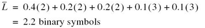
The entropy of the specified discrete memoryless source is calculated as follows (see (5.9)):

For this example, we may make two observations:
1. The average codeword length ![]() exceeds the entropy H(S) by only 3.67%.
exceeds the entropy H(S) by only 3.67%.
2. The average codeword length ![]() does indeed satisfy (5.23).
does indeed satisfy (5.23).

Figure 5.5 (a) Example of the Huffman encoding algorithm. (b) Source code.
It is noteworthy that the Huffman encoding process (i.e., the Huffman tree) is not unique. In particular, we may cite two variations in the process that are responsible for the nonuniqueness of the Huffman code. First, at each splitting stage in the construction of a Huffman code, there is arbitrariness in the way the symbols 0 and 1 are assigned to the last two source symbols. Whichever way the assignments are made, however, the resulting differences are trivial. Second, ambiguity arises when the probability of a combined symbol (obtained by adding the last two probabilities pertinent to a particular step) is found to equal another probability in the list. We may proceed by placing the probability of the new symbol as high as possible, as in Example 4. Alternatively, we may place it as low as possible. (It is presumed that whichever way the placement is made, high or low, it is consistently adhered to throughout the encoding process.) By this time, noticeable differences arise in that the codewords in the resulting source code can have different lengths. Nevertheless, the average codeword length remains the same.
As a measure of the variability in codeword lengths of a source code, we define the variance of the average codeword length ![]() over the ensemble of source symbols as
over the ensemble of source symbols as
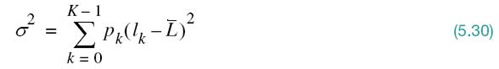
where p0, p1,…,pK – 1 are the source statistics and lk is the length of the codeword assigned to source symbol sk. It is usually found that when a combined symbol is moved as high as possible, the resulting Huffman code has a significantly smaller variance σ2 than when it is moved as low as possible. On this basis, it is reasonable to choose the former Huffman code over the latter.
Lempel-Ziv Coding
A drawback of the Huffman code is that it requires knowledge of a probabilistic model of the source; unfortunately, in practice, source statistics are not always known a priori. Moreover, in the modeling of text we find that storage requirements prevent the Huffman code from capturing the higher-order relationships between words and phrases because the codebook grows exponentially fast in the size of each super-symbol of letters (i.e., grouping of letters); the efficiency of the code is therefore compromised. To overcome these practical limitations of Huffman codes, we may use the Lempel–Ziv algorithm,7 which is intrinsically adaptive and simpler to implement than Huffman coding.
Basically, the idea behind encoding in the Lempel–Ziv algorithm is described as follows:
The source data stream is parsed into segments that are the shortest subsequences not encountered previously.
To illustrate this simple yet elegant idea, consider the example of the binary sequence
000101110010100101…
It is assumed that the binary symbols 0 and 1 are already stored in that order in the code book. We thus write
| Subsequences stored: | 0, 1 |
| Data to be parsed: | 000101110010100101… |
The encoding process begins at the left. With symbols 0 and 1 already stored, the shortest subsequence of the data stream encountered for the first time and not seen before is 00; so we write
| Subsequences stored: | 0, 1, 00 |
| Data to be parsed: | 0101110010100101… |
The second shortest subsequence not seen before is 01; accordingly, we go on to write
| Subsequences stored: | 0, 0, 00, 01 |
| Data to be parsed: | 01110010100101… |
The next shortest subsequence not encountered previously is 011; hence, we write
| Subsequences stored: | 0, 1, 00, 01, 011 |
| Data to be parsed: | 10010100101… |
We continue in the manner described here until the given data stream has been completely parsed. Thus, for the example at hand, we get the code book of binary subsequences shown in the second row of Figure 5.6.8
The first row shown in this figure merely indicates the numerical positions of the individual subsequences in the code book. We now recognize that the first subsequence of the data stream, 00, is made up of the concatenation of the first code book entry, 0, with itself; it is, therefore, represented by the number 11. The second subsequence of the data stream, 01, consists of the first code book entry, 0, concatenated with the second code book entry, 1; it is, therefore, represented by the number 12. The remaining subsequences are treated in a similar fashion. The complete set of numerical representations for the various subsequences in the code book is shown in the third row of Figure 5.6. As a further example illustrating the composition of this row, we note that the subsequence 010 consists of the concatenation of the subsequence 01 in position 4 and symbol 0 in position 1; hence, the numerical representation is 41. The last row shown in Figure 5.6 is the binary encoded representation of the different subsequences of the data stream.
The last symbol of each subsequence in the code book (i.e., the second row of Figure 5.6) is an innovation symbol, which is so called in recognition of the fact that its appendage to a particular subsequence distinguishes it from all previous subsequences stored in the code book. Correspondingly, the last bit of each uniform block of bits in the binary encoded representation of the data stream (i.e., the fourth row in Figure 5.6) represents the innovation symbol for the particular subsequence under consideration. The remaining bits provide the equivalent binary representation of the “pointer” to the root subsequence that matches the one in question, except for the innovation symbol.
The Lempel–Ziv decoder is just as simple as the encoder. Specifically, it uses the pointer to identify the root subsequence and then appends the innovation symbol. Consider, for example, the binary encoded block 1101 in position 9. The last bit, 1, is the innovation symbol. The remaining bits, 110, point to the root subsequence 10 in position 6. Hence, the block 1101 is decoded into 101, which is correct.
From the example described here, we note that, in contrast to Huffman coding, the Lempel–Ziv algorithm uses fixed-length codes to represent a variable number of source symbols; this feature makes the Lempel–Ziv code suitable for synchronous transmission.
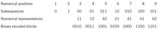
Figure 5.6 Illustrating the encoding process performed by the Lempel–Ziv algorithm on the binary sequence 000101110010100101…
In practice, fixed blocks of 12 bits long are used, which implies a code book of 212 = 4096 entries.
For a long time, Huffman coding was unchallenged as the algorithm of choice for lossless data compression; Huffman coding is still optimal, but in practice it is hard to implement. It is on account of practical implementation that the Lempel–Ziv algorithm has taken over almost completely from the Huffman algorithm. The Lempel–Ziv algorithm is now the standard algorithm for file compression.
5.5 Discrete Memoryless Channels
Up to this point in the chapter we have been preoccupied with discrete memoryless sources responsible for information generation. We next consider the related issue of information transmission. To this end, we start the discussion by considering a discrete memoryless channel, the counterpart of a discrete memoryless source.
A discrete memoryless channel is a statistical model with an input X and an output Y that is a noisy version of X; both X and Y are random variables. Every unit of time, the channel accepts an input symbol X selected from an alphabet ![]() and, in response, it emits an output symbol Y from an alphabet
and, in response, it emits an output symbol Y from an alphabet ![]() . The channel is said to be “discrete” when both of the alphabets
. The channel is said to be “discrete” when both of the alphabets ![]() and
and ![]() have finite sizes. It is said to be “memoryless” when the current output symbol depends only on the current input symbol and not any previous or future symbol.
have finite sizes. It is said to be “memoryless” when the current output symbol depends only on the current input symbol and not any previous or future symbol.
Figure 5.7a shows a view of a discrete memoryless channel. The channel is described in terms of an input alphabet
and an output alphabet
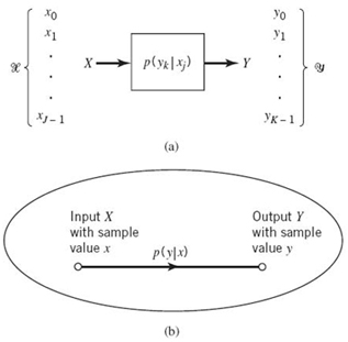
Figure 5.7 (a) Discrete memoryless channel; (b) Simplified graphical representation of the channel.
The cardinality of the alphabets ![]() and
and ![]() , or any other alphabet for that matter, is defined as the number of elements in the alphabet. Moreover, the channel is characterized by a set of transition probabilities
, or any other alphabet for that matter, is defined as the number of elements in the alphabet. Moreover, the channel is characterized by a set of transition probabilities
for which, according to probability theory, we naturally have
and
When the number of input symbols J and the number of output symbols K are not large, we may depict the discrete memoryless channel graphically in another way, as shown in Figure 5.7b. In this latter depiction, each input–output symbol pair (x, y), characterized by the transition probability p(y|x) > 0, is joined together by a line labeled with the number p(y|x).
Also, the input alphabet ![]() and output alphabet
and output alphabet ![]() need not have the same size; hence the use of J for the size of
need not have the same size; hence the use of J for the size of ![]() and K for the size of
and K for the size of ![]() . For example, in channel coding, the size K of the output alphabet
. For example, in channel coding, the size K of the output alphabet ![]() may be larger than the size J of the input alphabet
may be larger than the size J of the input alphabet ![]() ; thus, K ≥ J. On the other hand, we may have a situation in which the channel emits the same symbol when either one of two input symbols is sent, in which case we have K ≤ J.
; thus, K ≥ J. On the other hand, we may have a situation in which the channel emits the same symbol when either one of two input symbols is sent, in which case we have K ≤ J.
A convenient way of describing a discrete memoryless channel is to arrange the various transition probabilities of the channel in the form of a matrix
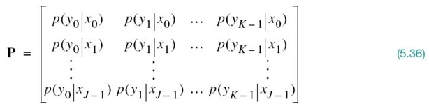
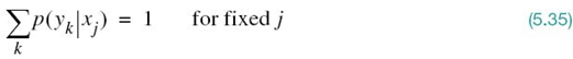
The J-by-K matrix P is called the channel matrix, or stochastic matrix. Note that each row of the channel matrix P corresponds to a fixed channel input, whereas each column of the matrix corresponds to a fixed channel output. Note also that a fundamental property of the channel matrix P, as defined here, is that the sum of the elements along any row of the stochastic matrix is always equal to one, according to (5.35).
Suppose now that the inputs to a discrete memoryless channel are selected according to the probability distribution {p(xj), j = 0, 1,…,J – 1}. In other words, the event that the channel input X = xj occurs with probability
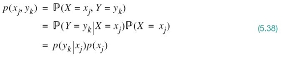
Having specified the random variable X denoting the channel input, we may now specify the second random variable Y denoting the channel output. The joint probability distribution of the random variables X and Y is given by
The marginal probability distribution of the output random variable Y is obtained by averaging out the dependence of p(xj, yk) on xj, obtaining

The probabilities p(xj) for j = 0, 1,…,J – 1, are known as the prior probabilities of the various input symbols. Equation (5.39) states:
If we are given the input prior probabilities p(xj) and the stochastic matrix (i.e., the matrix of transition probabilities p(yk|xj)), then we may calculate the probabilities of the various output symbols, the p(yk).
EXAMPLE 5 Binary Symmetric Channel
The binary symmetric channel is of theoretical interest and practical importance. It is a special case of the discrete memoryless channel with J = K = 2. The channel has two input symbols (x0 = 0, x1 = 1) and two output symbols (y0 = 0, y1 = 1). The channel is symmetric because the probability of receiving 1 if 0 is sent is the same as the probability of receiving 0 if 1 is sent. This conditional probability of error is denoted by p (i.e., the probability of a bit flipping). The transition probability diagram of a binary symmetric channel is as shown in Figure 5.8. Correspondingly, we may express the stochastic matrix as


Figure 5.8 Transition probability diagram of binary symmetric channel.
5.6 Mutual Information
Given that we think of the channel output Y (selected from alphabet ![]() ) as a noisy version of the channel input X (selected from alphabet
) as a noisy version of the channel input X (selected from alphabet ![]() ) and that the entropy H(X) is a measure of the prior uncertainty about X, how can we measure the uncertainty about X after observing Y? To answer this basic question, we extend the ideas developed in Section 5.2 by defining the conditional entropy of X selected from alphabet
) and that the entropy H(X) is a measure of the prior uncertainty about X, how can we measure the uncertainty about X after observing Y? To answer this basic question, we extend the ideas developed in Section 5.2 by defining the conditional entropy of X selected from alphabet ![]() , given Y = yk. Specifically, we write
, given Y = yk. Specifically, we write
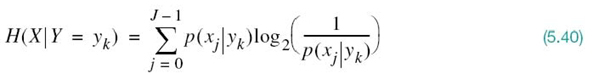
This quantity is itself a random variable that takes on the values H(X|Y = y0),…,H(X|Y = yK – 1) with probabilities p(y0),…,p(yK – 1), respectively. The expectation of entropy H(X|Y = yk) over the output alphabet ![]() is therefore given by
is therefore given by
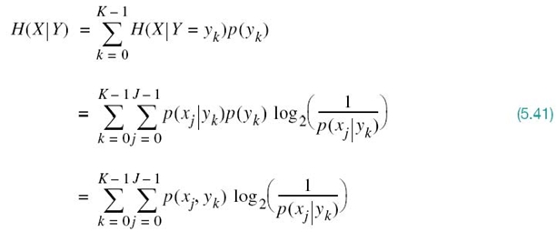
where, in the last line, we used the definition of the probability of the joint event (X = xj, Y = yk) as shown by
The quantity H(X|Y) in (5.41) is called the conditional entropy, formally defined as follows:
The conditional entropy, H(X|Y), is the average amount of uncertainty remaining about the channel input after the channel output has been observed.
The conditional entropy H(X|Y) relates the channel output Y to the channel input X. The entropy H(X) defines the entropy of the channel input X by itself. Given these two entropies, we now introduce the definition
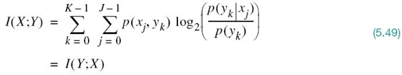
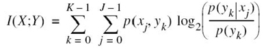
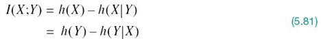
which is called the mutual information of the channel. To add meaning to this new concept, we recognize that the entropy H(X) accounts for the uncertainty about the channel input before observing the channel output and the conditional entropy H(X|Y) accounts for the uncertainty about the channel input after observing the channel output. We may, therefore, go on to make the statement:
The mutual information I(X;Y) is a measure of the uncertainty about the channel input, which is resolved by observing the channel output.
Equation (5.43) is not the only way of defining the mutual information of a channel. Rather, we may define it in another way, as shown by
on the basis of which we may make the next statement:
The mutual information I(Y;X) is a measure of the uncertainty about the channel output that is resolved by sending the channel input.
On first sight, the two definitions of (5.43) and (5.44) look different. In reality, however, they embody equivalent statements on the mutual information of the channel that are worded differently. More specifically, they could be used interchangeably, as demonstrated next.
Properties of Mutual Information
PROPERTY 1 Symmetry
The mutual information of a channel is symmetric in the sense that
To prove this property, we first use the formula for entropy and then use (5.35) and (5.38), in that order, obtaining

where, in going from the third to the final line, we made use of the definition of a joint probability. Hence, substituting (5.41) and (5.46) into (5.43) and then combining terms, we obtain

Note that the double summation on the right-hand side of (5.47) is invariant with respect to swapping the x and y. In other words, the symmetry of the mutual information I(X;Y) is already evident from (5.47).
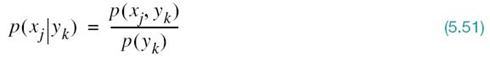
To further confirm this property, we may use Bayes’ rule for conditional probabilities, previously discussed in Chapter 3, to write

Hence, substituting (5.48) into (5.47) and interchanging the order of summation, we get
which proves property1.
PROPERTY 2 Nonnegativity
The mutual information is always nonnegative; that is;
To prove this property, we first note from (5.42) that
Hence, substituting (5.51) into (5.47), we may express the mutual information of the channel as

Next, a direct application of the fundamental inequality of (5.12) on relative entropy confirms (5.50), with equality if, and only if,
In words, property 2 states the following:
We cannot lose information, on the average, by observing the output of a channel.
Moreover, the mutual information is zero if, and only if, the input and output symbols of the channel are statistically independent; that is, when (5.53) is satisfied.
PROPERTY 3 Expansion of the Mutual Information
The mutual information of a channel is related to the joint entropy of the channel input and channel output by
where the joint entropy H(X, Y) is defined by
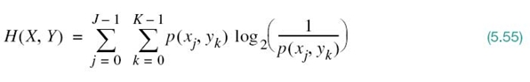
To prove (5.54), we first rewrite the joint entropy in the equivalent form
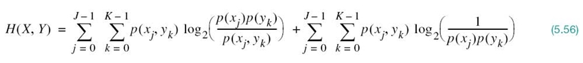
The first double summation term on the right-hand side of (5.56) is recognized as the negative of the mutual information of the channel, I(X;Y), previously given in (5.52). As for the second summation term, we manipulate it as follows:
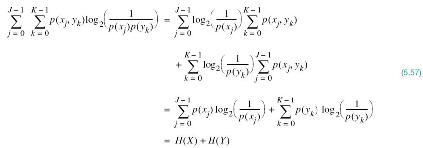
where, in the first line, we made use of the following relationship from probability theory:
and a similar relationship holds for the second line of the equation.
Accordingly, using (5.52) and (5.57) in (5.56), we get the result
which, on rearrangement, proves Property 3.
We conclude our discussion of the mutual information of a channel by providing a diagramatic interpretation in Figure 5.9 of (5.43), (5.44), and (5.54).

Figure 5.9 Illustrating the relations among various channel entropies.
5.7 Channel Capacity
The concept of entropy introduced in Section 5.2 prepared us for formulating Shannon’s first theorem: the source-coding theorem. To set the stage for formulating Shannon’s second theorem, namely the channel-coding theorem, this section introduces the concept of capacity, which, as mentioned previously, defines the intrinsic ability of a communication channel to convey information.
To proceed, consider a discrete memoryless channel with input alphabet ![]() , output alphabet
, output alphabet ![]() , and transition probabilities p(yk|xj), where j = 0, 1,…,J – 1 and k = 0, 1,…,K – 1. The mutual information of the channel is defined by the first line of (5.49), which is reproduced here for convenience:
, and transition probabilities p(yk|xj), where j = 0, 1,…,J – 1 and k = 0, 1,…,K – 1. The mutual information of the channel is defined by the first line of (5.49), which is reproduced here for convenience:
where, according to (5.38),
![]()
Also, from (5.39), we have

Putting these three equations into a single equation, we write

Careful examination of the double summation in this equation reveals two different probabilities, on which the essence of mutual information I(X;Y) depends:
- the probability distribution
 that characterizes the channel input and
 - the transition probability distribution
 that characterizes the channel itself.
These two probability distributions are obviously independent of each other. Thus, given a channel characterized by the transition probability distribution {p(yk|xj}, we may now introduce the channel capacity, which is formally defined in terms of the mutual information between the channel input and output as follows:

The maximization in (5.59) is performed, subject to two input probabilistic constraints:
![]()
Accordingly, we make the following statement:
The channel capacity of a discrete memoryless channel, commonly denoted by C, is defined as the maximum mutual information I(X;Y) in any single use of the channel (i.e., signaling interval), where the maximization is over all possible input probability distributions {p(xj)} on X.
The channel capacity is clearly an intrinsic property of the channel.
EXAMPLE 6 Binary Symmetric Channel (Revisited)
Consider again the binary symmetric channel, which is described by the transition probability diagram of Figure 5.8. This diagram is uniquely defined by the conditional probability of error p.
From Example 1 we recall that the entropy H(X) is maximized when the channel input probability p(x0) = p(x1) = 1/2, where x0 and x1 are each 0 or 1. Hence, invoking the defining equation (5.59), we find that the mutual information I(X;Y) is similarly maximized and thus write
![]()
From Figure 5.8 we have
![]()
and
![]()
Therefore, substituting these channel transition probabilities into (5.49) with J = K = 2 and then setting the input probability p(x0) = p(x1) = 1/2 in (5.59), we find that the capacity of the binary symmetric channel is
![]()
Moreover, using the definition of the entropy function introduced in (5.16), we may reduce (5.60) to
![]()
The channel capacity C varies with the probability of error (i.e., transition probability) p in a convex manner as shown in Figure 5.10, which is symmetric about p = 1/2. Comparing the curve in this figure with that in Figure 5.2, we make two observations:
1. When the channel is noise free, permitting us to set p = 0, the channel capacity C attains its maximum value of one bit per channel use, which is exactly the information in each channel input. At this value of p, the entropy function H(p) attains its minimum value of zero.
2. When the conditional probability of error p = 1/2 due to channel noise, the channel capacity C attains its minimum value of zero, whereas the entropy function H(p) attains its maximum value of unity; in such a case, the channel is said to be useless in the sense that the channel input and output assume statistically independent structures.
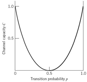
Figure 5.10 Variation of channel capacity of a binary symmetric channel with transition probability p.
5.8 Channel-coding Theorem
With the entropy of a discrete memoryless source and the corresponding capacity of a discrete memoryless channel at hand, we are now equipped with the concepts needed for formulating Shannon’s second theorem: the channel-coding theorem.
To this end, we first recognize that the inevitable presence of noise in a channel causes discrepancies (errors) between the output and input data sequences of a digital communication system. For a relatively noisy channel (e.g., wireless communication channel), the probability of error may reach a value as high as 10–1, which means that (on the average) only 9 out of 10 transmitted bits are received correctly. For many applications, this level of reliability is utterly unacceptable. Indeed, a probability of error equal to 10–6 or even lower is often a necessary practical requirement. To achieve such a high level of performance, we resort to the use of channel coding.
The design goal of channel coding is to increase the resistance of a digital communication system to channel noise. Specifically, channel coding consists of mapping the incoming data sequence into a channel input sequence and inverse mapping the channel output sequence into an output data sequence in such a way that the overall effect of channel noise on the system is minimized. The first mapping operation is performed in the transmitter by a channel encoder, whereas the inverse mapping operation is performed in the receiver by a channel decoder, as shown in the block diagram of Figure 5.11; to simplify the exposition, we have not included source encoding (before channel encoding) and source decoding (after channel decoding) in this figure.9

Figure 5.11 Block diagram of digital communication system.
The channel encoder and channel decoder in Figure 5.11 are both under the designer’s control and should be designed to optimize the overall reliability of the communication system. The approach taken is to introduce redundancy in the channel encoder in a controlled manner, so as to reconstruct the original source sequence as accurately as possible. In a rather loose sense, we may thus view channel coding as the dual of source coding, in that the former introduces controlled redundancy to improve reliability whereas the latter reduces redundancy to improve efficiency.
Treatment of the channel-coding techniques is deferred to Chapter 10. For the purpose of our present discussion, it suffices to confine our attention to block codes. In this class of codes, the message sequence is subdivided into sequential blocks each k bits long, and each k-bit block is mapped into an n-bit block, where n > k. The number of redundant bits added by the encoder to each transmitted block is n – k bits. The ratio k/n is called the code rate. Using r to denote the code rate, we write
where, of course, r is less than unity. For a prescribed k, the code rate r (and, therefore, the system’s coding efficiency) approaches zero as the block length n approaches infinity.
The accurate reconstruction of the original source sequence at the destination requires that the average probability of symbol error be arbitrarily low. This raises the following important question:
Does a channel-coding scheme exist such that the probability that a message bit will be in error is less than any positive number ε (i.e., as small as we want it), and yet the channel-coding scheme is efficient in that the code rate need not be too small?
The answer to this fundamental question is an emphatic “yes.” Indeed, the answer to the question is provided by Shannon’s second theorem in terms of the channel capacity C, as described in what follows.
Up until this point, time has not played an important role in our discussion of channel capacity. Suppose then the discrete memoryless source in Figure 5.11 has the source alphabet ![]() and entropy H(S) bits per source symbol. We assume that the source emits symbols once every Ts seconds. Hence, the average information rate of the source is H(S)/Ts bits per second. The decoder delivers decoded symbols to the destination from the source alphabet S and at the same source rate of one symbol every Ts seconds. The discrete memoryless channel has a channel capacity equal to C bits per use of the channel. We assume that the channel is capable of being used once every Tc seconds. Hence, the channel capacity per unit time is C/Tc bits per second, which represents the maximum rate of information transfer over the channel. With this background, we are now ready to state Shannon’s second theorem, the channel-coding theorem,10 in two parts as follows:
and entropy H(S) bits per source symbol. We assume that the source emits symbols once every Ts seconds. Hence, the average information rate of the source is H(S)/Ts bits per second. The decoder delivers decoded symbols to the destination from the source alphabet S and at the same source rate of one symbol every Ts seconds. The discrete memoryless channel has a channel capacity equal to C bits per use of the channel. We assume that the channel is capable of being used once every Tc seconds. Hence, the channel capacity per unit time is C/Tc bits per second, which represents the maximum rate of information transfer over the channel. With this background, we are now ready to state Shannon’s second theorem, the channel-coding theorem,10 in two parts as follows:
1. Let a discrete memoryless source with an alphabet ![]() have entropy H(S) for random variable S and produce symbols once every Ts seconds. Let a discrete memoryless channel have capacity C and be used once every Tc seconds, Then, if
have entropy H(S) for random variable S and produce symbols once every Ts seconds. Let a discrete memoryless channel have capacity C and be used once every Tc seconds, Then, if
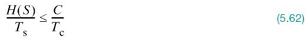
there exists a coding scheme for which the source output can be transmitted over the channel and be reconstructed with an arbitrarily small probability of error. The parameter C/Tc is called the critical rate; when (5.62) is satisfied with the equality sign, the system is said to be signaling at the critical rate.
2. Conversely, if
![]()
it is not possible to transmit information over the channel and reconstruct it with an arbitrarily small probability of error.
The channel-coding theorem is the single most important result of information theory. The theorem specifies the channel capacity C as a fundamental limit on the rate at which the transmission of reliable error-free messages can take place over a discrete memoryless channel. However, it is important to note two limitations of the theorem:
1. The channel-coding theorem does not show us how to construct a good code. Rather, the theorem should be viewed as an existence proof in the sense that it tells us that if the condition of (5.62) is satisfied, then good codes do exist. Later, in Chapter10, we describe good codes for discrete memoryless channels.
2. The theorem does not have a precise result for the probability of symbol error after decoding the channel output. Rather, it tells us that the probability of symbol error tends to zero as the length of the code increases, again provided that the condition of (5.62) is satisfied.
Application of the Channel-coding Theorem to Binary Symmetric Channels
Consider a discrete memoryless source that emits equally likely binary symbols (0s and 1s) once every Ts seconds. With the source entropy equal to one bit per source symbol (see Example 1), the information rate of the source is (1/Ts) bits per second. The source sequence is applied to a channel encoder with code rate r. The channel encoder produces a symbol once every Tc seconds. Hence, the encoded symbol transmission rate is (1/Tc) symbols per second. The channel encoder engages a binary symmetric channel once every Tc seconds. Hence, the channel capacity per unit time is (C/Tc) bits per second, where C is determined by the prescribed channel transition probability p in accordance with (5.60). Accordingly, part (1) of the channel-coding theorem implies that if

then the probability of error can be made arbitrarily low by the use of a suitable channel-encoding scheme. But the ratio Tc/Ts equals the code rate of the channel encoder:

Hence, we may restate the condition of (5.63) simply as
r ≤ C
That is, for r ≤ C, there exists a code (with code rate less than or equal to channel capacity C) capable of achieving an arbitrarily low probability of error.
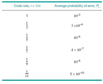
EXAMPLE 7 Repetition Code
In this example we present a graphical interpretation of the channel-coding theorem. We also bring out a surprising aspect of the theorem by taking a look at a simple coding scheme.
Consider first a binary symmetric channel with transition probability p = 10–2. For this value of p, we find from (5.60) that the channel capacity C = 0.9192. Hence, from the channel-coding theorem, we may state that, for any ε > 0 and r ≤ 0.9192, there exists a code of large enough length n, code rate r, and an appropriate decoding algorithm such that, when the coded bit stream is sent over the given channel, the average probability of channel decoding error is less than ε. This result is depicted in Figure 5.12 for the limiting value ε = 10–8.
To put the significance of this result in perspective, consider next a simple coding scheme that involves the use of a repetition code, in which each bit of the message is repeated several times. Let each bit (0 or 1) be repeated n times, where n = 2m + 1 is an odd integer. For example, for n = 3, we transmit 0 and 1 as 000 and 111, respectively. Intuitively, it would seem logical to use a majority rule for decoding, which operates as follows:
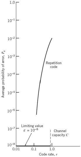
Figure 5.12 Illustrating the significance of the channel-coding theorem.
If in a block of n repeated bits (representing one bit of the message) the number of 0s exceeds the number of 1s, the decoder decides in favor of a 0; otherwise, it decides in favor of a 1.
Hence, an error occurs when m + 1 or more bits out of n = 2m + 1 bits are received incorrectly. Because of the assumed symmetric nature of the channel, the average probability of error, denoted by Pe, is independent of the prior probabilities of 0 and 1. Accordingly, we find that Pe is given by

where p is the transition probability of the channel.
Table 5.3 gives the average probability of error Pe for a repetition code that is calculated by using (5.65) for different values of the code rate r. The values given here assume the use of a binary symmetric channel with transition probability p = 10–2. The improvement in reliability displayed in Table 5.3 is achieved at the cost of decreasing code rate. The results of this table are also shown plotted as the curve labeled “repetition code” in Figure 5.12. This curve illustrates the exchange of code rate for message reliability, which is a characteristic of repetition codes.
This example highlights the unexpected result presented to us by the channel-coding theorem. The result is that it is not necessary to have the code rate r approach zero (as in the case of repetition codes) to achieve more and more reliable operation of the communication link. The theorem merely requires that the code rate be less than the channel capacity C.
Table 5.3 Average probability of error for repetition code
5.9 Differential Entropy and Mutual Information for Continuous Random Ensembles
The sources and channels considered in our discussion of information-theoretic concepts thus far have involved ensembles of random variables that are discrete in amplitude. In this section, we extend these concepts to continuous random variables. The motivation for doing so is to pave the way for the description of another fundamental limit in information theory, which we take up in Section 5.10.
Consider a continuous random variable X with the probability density function fX(x). By analogy with the entropy of a discrete random variable, we introduce the following definition:
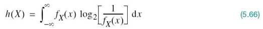
We refer to the new term h(X) as the differential entropy of X to distinguish it from the ordinary or absolute entropy. We do so in recognition of the fact that, although h(X) is a useful mathematical quantity to know, it is not in any sense a measure of the randomness of X. Nevertheless, we justify the use of (5.66) in what follows. We begin by viewing the continuous random variable X as the limiting form of a discrete random variable that assumes the value xk = kΔx, where k = 0, ±1, ±2,…, and Δx approaches zero. By definition, the continuous random variable X assumes a value in the interval [xk, xk + Δx] with probability fX(xk)Δx. Hence, permitting Δx to approach zero, the ordinary entropy of the continuous random variable X takes the limiting form
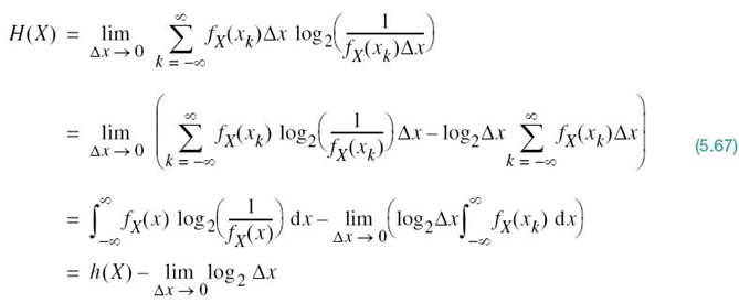
In the last line of (5.67), use has been made of (5.66) and the fact that the total area under the curve of the probability density function fX(x) is unity. In the limit as Δx approaches zero, the term –log2Δx approaches infinity. This means that the entropy of a continuous random variable is infinitely large. Intuitively, we would expect this to be true because a continuous random variable may assume a value anywhere in the interval (–∞, ∞); we may, therefore, encounter uncountable infinite numbers of probable outcomes. To avoid the problem associated with the term log2Δx, we adopt h(X) as a differential entropy, with the term –log2Δx serving merely as a reference. Moreover, since the information transmitted over a channel is actually the difference between two entropy terms that have a common reference, the information will be the same as the difference between the corresponding differential entropy terms. We are, therefore, perfectly justified in using the term h(X), defined in (5.66), as the differential entropy of the continuous random variable X.
When we have a continuous random vector X consisting of n random variables X1, X2,…,Xn, we define the differential entropy of X as the n-fold integral

where fX(x) is the joint probability density function of X.
EXAMPLE 8 Uniform Distribution
To illustrate the notion of differential entropy, consider a random variable X uniformly distributed over the interval (0, a). The probability density function of X is
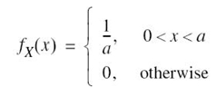
Applying (5.66) to this distribution, we get

Note that loga < 0 for a < 1. Thus, this example shows that, unlike a discrete random variable, the differential entropy of a continuous random variable can assume a negative value.
Relative Entropy of Continuous Distributions
In (5.12) we defined the relative entropy of a pair of different discrete distributions. To extend that definition to a pair of continuous distributions, consider the continuous random variables X and Y whose respective probability density functions are denoted by fX(x) and fY(x) for the same sample value (argument) x. The relative entropy11 of the random variables X and Y is defined by
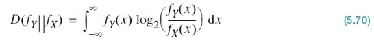
where fX(x) is viewed as the “reference” distribution. In a corresponding way to the fundamental property of (5.13), we have
Combining (5.70) and (5.71) into a single inequality, we may thus write
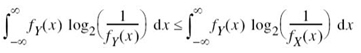
The expression on the left-hand side of this inequality is recognized as the differential entropy of the random variable Y, namely h(Y). Accordingly,

The next example illustrates an insightful application of (5.72).
EXAMPLE 9 Gaussian Distribution
Suppose two random variables, X and Y, are described as follows:
- the random variables X and Y have the common mean μ and variance σ2;
- the random variable X is Gaussian distributed (see Section 3.9) as shown by

Hence, substituting (5.73) into (5.72) and changing the base of the logarithm from 2 to e = 2.7183, we get
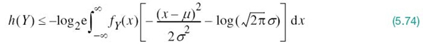
where e is the base of the natural algorithm. We now recognize the following characterizations of the random variable Y (given that its mean is μ and its variance is σ2):

We may, therefore, simplify (5.74) as
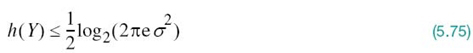
The quantity on the right-hand side of (5.75) is, in fact, the differential entropy of the Gaussian random variable X:
Finally, combining (5.75) and (5.76), we may write
where equality holds if, and only if, Y = X.
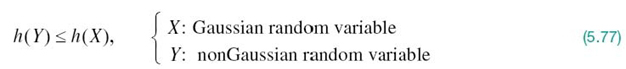
We may now summarize the results of this important example by describing two entropic properties of a random variable:
PROPERTY 1 For any finite variance, a Gaussian random variable has the largest differential entropy attainable by any other random variable.
PROPERTY 2 The entropy of a Gaussian random variable is uniquely determined by its variance (i.e., the entropy is independent of the mean).
Indeed, it is because of property 1 that the Gaussian channel model is so widely used as a conservative model in the study of digital communication systems.
Mutual Information
Continuing with the information-theoretic characterization of continuous random variables, we may use analogy with (5.47) to define the mutual information between the pair of continuous random variables X and Y as follows:

where fX, Y(x, y) is the joint probability density function of X and Y and fX(x|y) is the conditional probability density function of X given Y = y. Also, by analogy with (5.45), (5.50), (5.43), and (5.44), we find that the mutual information between the pair of Gausian random variables has the following properties:
The parameter h(X) is the differential entropy of X; likewise for h(Y). The parameter h(X|Y) is the conditional differential entropy of X given Y; it is defined by the double integral (see (5.41))

The parameter h(Y|X) is the conditional differential entropy of Y given X; it is defined in a manner similar to h(X|Y).
5.10 Information Capacity Law
In this section we use our knowledge of probability theory to expand Shannon’s channel-coding theorem, so as to formulate the information capacity for a band-limited, power-limited Gaussian channel, depicted in Figure 5.13. To be specific, consider a zero-mean stationary process X(t) that is band-limited to B hertz. Let Xk, k = 1,2,…,K, denote the continuous random variables obtained by uniform sampling of the process X(t) at a rate of 2B samples per second. The rate 2B samples per second is the smallest permissible rate for a bandwidth B that would not result in a loss of information in accordance with the sampling theorem; this is discussed in Chapter 6. Suppose that these samples are transmitted in T seconds over a noisy channel, also band-limited to B hertz. Hence, the total number of samples K is given by
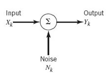
Figure 5.13 Model of discrete-time, memoryless Gaussian channel.
We refer to Xk as a sample of the transmitted signal. The channel output is perturbed by additive white Gaussian noise (AWGN) of zero mean and power spectral density N0/2. The noise is band-limited to B hertz. Let the continuous random variables Yk, k = 1, 2,.., K, denote the corresponding samples of the channel output, as shown by
The noise sample Nk in (5.84) is Gaussian with zero mean and variance
We assume that the samples Yk, k = 1,2,…,K, are statistically independent.
A channel for which the noise and the received signal are as described in (5.84) and (5.85) is called a discrete-time, memoryless Gaussian channel, modeled as shown in Figure 5.13. To make meaningful statements about the channel, however, we have to assign a cost to each channel input. Typically, the transmitter is power limited; therefore, it is reasonable to define the cost as
where P is the average transmitted power. The power-limited Gaussian channel described herein is not only of theoretical importance but also of practical importance, in that it models many communication channels, including line-of-sight radio and satellite links.
The information capacity of the channel is defined as the maximum of the mutual information between the channel input Xk and the channel output Yk over all distributions of the input Xk that satisfy the power constraint of (5.86). Let I(Xk;Yk) denote the mutual information between Xk and Yk. We may then define the information capacity of the channel as

In words, maximization of the mutual information I(Xk;Yk) is done with respect to all probability distributions of the channel input Xk, satisfying the power constraint ![]() .
.
The mutual information I(Xk;Yk) can be expressed in one of the two equivalent forms shown in (5.81). For the purpose at hand, we use the second line of this equation to write
Since Xk and Nk are independent random variables and their sum equals Yk in accordance with (5.84), we find that the conditional differential entropy of Yk given Xk is equal to the differential entropy of Nk, as shown by
Hence, we may rewrite (5.88) as
With h(Nk) being independent of the distribution of Xk, it follows that maximizing I(Xk;Yk) in accordance with (5.87) requires maximizing the differential entropy h(Yk). For h(Yk) to be maximum, Yk has to be a Gaussian random variable. That is to say, samples of the channel output represent a noiselike process. Next, we observe that since Nk is Gaussian by assumption, the sample Xk of the channel input must be Gaussian too. We may therefore state that the maximization specified in (5.87) is attained by choosing samples of the channel input from a noiselike Gaussian-distributed process of average power P. Correspondingly, we may reformulate (5.87) as
where the mutual information I(Xk;Yk) is defined in accordance with (5.90).
For evaluation of the information capacity C, we now proceed in three stages:
1. The variance of sample Yk of the channel output equals P + σ2, which is a consequence of the fact that the random variables X and N are statistically independent; hence, the use of (5.76) yields the differential entropy

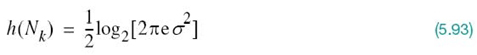
2. The variance of the noisy sample Nk equals σ2; hence, the use of (5.76) yields the differential entropy
3. Substituting (5.92) and (5.93) into (5.90), and recognizing the definition of information capacity given in (5.91), we get the formula:
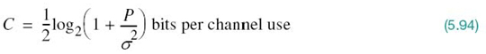
With the channel used K times for the transmission of K samples of the process X(t) in T seconds, we find that the information capacity per unit time is (K/T) times the result given in (5.94). The number K equals 2BT, as in (5.83). Accordingly, we may express the information capacity of the channel in the following equivalent form:
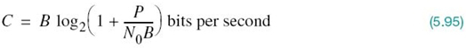
where N0B is the total noise power at the channel output, defined in accordance with (5.85).
Based on the formula of (5.95), we may now make the following statement
The information capacity of a continuous channel of bandwidth B hertz, perturbed by AWGN of power spectral density N0/2 and limited in bandwidth to B, is given by the formula
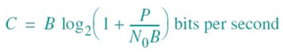
where P is the average transmitted power.
The information capacity law12 of (5.95) is one of the most remarkable results of Shannon’s information theory. In a single formula, it highlights most vividly the interplay among three key system parameters: channel bandwidth, average transmitted power, and power spectral density of channel noise. Note, however, that the dependence of information capacity C on channel bandwidth B is linear, whereas its dependence on signal-to-noise ratio P/(N0B) is logarithmic. Accordingly, we may make another insightful statement:
It is easier to increase the information capacity of a continuous communication channel by expanding its bandwidth than by increasing the transmitted power for a prescribed noise variance.
The information capacity formula implies that, for given average transmitted power P and channel bandwidth B, we can transmit information at the rate of C bits per second, as defined in (5.95), with arbitrarily small probability of error by employing a sufficiently complex encoding system. It is not possible to transmit at a rate higher than C bits per second by any encoding system without a definite probability of error. Hence, the channel capacity law defines the fundamental limit on the permissible rate of error-free transmission for a power-limited, band-limited Gaussian channel. To approach this limit, however, the transmitted signal must have statistical properties approximating those of white Gaussian noise.
Sphere Packing
To provide a plausible argument supporting the information capacity law, suppose that we use an encoding scheme that yields K codewords, one for each sample of the transmitted signal. Let n denote the length (i.e., the number of bits) of each codeword. It is presumed that the coding scheme is designed to produce an acceptably low probability of symbol error. Furthermore, the codewords satisfy the power constraint; that is, the average power contained in the transmission of each codeword with n bits is nP, where P is the average power per bit.
Suppose that any codeword in the code is transmitted. The received vector of n bits is Gaussian distributed with a mean equal to the transmitted codeword and a variance equal to nσ2, where σ2 is the noise variance. With a high probability, we may say that the received signal vector at the channel output lies inside a sphere of radius ![]() ; that is, centered on the transmitted codeword. This sphere is itself contained in a larger sphere of radius
; that is, centered on the transmitted codeword. This sphere is itself contained in a larger sphere of radius ![]() , where n(P + σ2) is the average power of the received signal vector.
, where n(P + σ2) is the average power of the received signal vector.
We may thus visualize the sphere packing13 as portrayed in Figure 5.14. With everything inside a small sphere of radius ![]() assigned to the codeword on which it is centered. It is therefore reasonable to say that, when this particular codeword is transmitted, the probability that the received signal vector will lie inside the correct “decoding” sphere is high. The key question is:
assigned to the codeword on which it is centered. It is therefore reasonable to say that, when this particular codeword is transmitted, the probability that the received signal vector will lie inside the correct “decoding” sphere is high. The key question is:

Figure 5.14 The sphere-packing problem.
How many decoding spheres can be packed inside the larger sphere of received signal vectors? In other words, how many codewords can we in fact choose?
To answer this question, we want to eliminate the overlap between the decoding spheres as depicted in Figure 5.14. Moreover, expressing the volume of an n-dimensional sphere of radius r as Anrn, where An is a scaling factor, we may go on to make two statements:
1. The volume of the sphere of received signal vectors is An[n(P + σ2)]n/2.
2. The volume of the decoding sphere is An(nσ2)n/2.
Accordingly, it follows that the maximum number of nonintersecting decoding spheres that can be packed inside the sphere of possible received signal vectors is given by
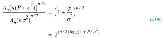
Taking the logarithm of this result to base 2, we readily see that the maximum number of bits per transmission for a low probability of error is indeed as defined previously in (5.94).
A final comment is in order: (5.94) is an idealized manifestation of Shannon’s channel-coding theorem, in that it provides an upper bound on the physically realizable information capacity of a communication channel.
5.11 Implications of the Information Capacity Law
Now that we have a good understanding of the information capacity law, we may go on to discuss its implications in the context of a Gaussian channel that is limited in both power and bandwidth. For the discussion to be useful, however, we need an ideal framework against which the performance of a practical communication system can be assessed. To this end, we introduce the notion of an ideal system, defined as a system that transmits data at a bit rate Rb equal to the information capacity C. We may then express the average transmitted power as
where Eb is the transmitted energy per bit. Accordingly, the ideal system is defined by the equation
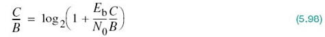
Rearranging this formula, we may define the signal energy-per-bit to noise power spectral density ratio, Eb/N0, in terms of the ratio C/B for the ideal system as follows:

A plot of the bandwidth efficiency Rb/B versus Eb/N0 is called the bandwidth-efficiency diagram. A generic form of this diagram is displayed in Figure 5.15, where the curve labeled “capacity boundary” corresponds to the ideal system for which Rb = C.

Figure 5.15 Bandwidth-efficiency diagram.
Based on Figure 5.15, we can make three observations:
1. For infinite channel bandwidth, the ratio Eb/N0 approaches the limiting value
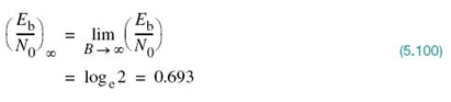
where loge stands for the natural logarithm ln. The value defined in (5.100) is called the Shannon limit for an AWGN channel, assuming a code rate of zero. Expressed in decibels, the Shannon limit equals –1.6 dB. The corresponding limiting value of the channel capacity is obtained by letting the channel bandwidth B in (5.95) approach infinity, in which case we obtain
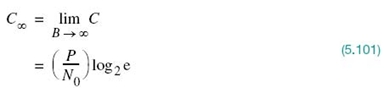
2. The capacity boundary is defined by the curve for the critical bit rate Rb = C. For any point on this boundary, we may flip a fair coin (with probability of 1/2) whether we have error-free transmission or not. As such, the boundary separates combinations of system parameters that have the potential for supporting error-free transmission (Rb > C) from those for which error-free transmission is not possible (Rb < C). The latter region is shown shaded in Figure 5.15.
3. The diagram highlights potential trade-offs among three quantities: the Eb/N0, the ratio Rb/B, and the probability of symbol error Pe. In particular, we may view movement of the operating point along a horizontal line as trading Pe versus Eb/N0 for a fixed Rb/B. On the other hand, we may view movement of the operating point along a vertical line as trading Pe versus Rb/B for a fixed Eb/N0.
EXAMPLE 10 Capacity of Binary-Input AWGN Channel
In this example, we investigate the capacity of an AWGN channel using encoded binary antipodal signaling (i.e., levels –1 and +1 for binary symbols 0 and 1, respectively). In particular, we address the issue of determining the minimum achievable bit error rate as a function of Eb/N0 for varying code rate r. It is assumed that the binary symbols 0 and 1 are equiprobable.
Let the random variables X and Y denote the channel input and channel output respectively; X is a discrete variable, whereas Y is a continuous variable. In light of the second line of (5.81), we may express the mutual information between the channel input and channel output as
![]()
The second term, h(Y|X), is the conditional differential entropy of the channel output Y, given the channel input X. By virtue of (5.89) and (5.93), this term is just the entropy of a Gaussian distribution. Hence, using σ2 to denote the variance of the channel noise, we write
![]()
Next, the first term, h(Y), is the differential entropy of the channel output Y. With the use of binary antipodal signaling, the probability density function of Y, given X = x, is a mixture of two Gaussian distributions with common variance σ2 and mean values –1 and +1, as shown by
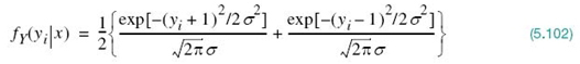
Hence, we may determine the differential entropy of Y using the formula
![]()
where fY(yi | x) is defined by (5.102). From the formulas of h(Y|X) and h(Y), it is clear that the mutual information is solely a function of the noise variance σ2. Using M(σ2) to denote this functional dependence, we may thus write
![]()
Unfortunately, there is no closed formula that we can derive for M(σ2) because of the difficulty of determining h(Y). Nevertheless, the differential entropy h(Y) can be well approximated using Monte Carlo integration; see Appendix E for details.
Because symbols 0 and 1 are equiprobable, it follows that the channel capacity C is equal to the mutual information between X and Y. Hence, for error-free data transmission over the AWGN channel, the code rate r must satisfy the condition
A robust measure of the ratio Eb/N0, is
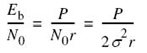
where P is the average transmitted power and N0/2 is the two-sided power spectral density of the channel noise. Without loss of generality, we may set P = 1. We may then express the noise variance as
Substituting Equation (5.104) into (5.103) and rearranging terms, we get the desired relation:

where M–1(r) is the inverse of the mutual information between the channel input and putput, expressed as a function of the code rate r.
Using the Monte Carlo method to estimate the differential entropy h(Y) and therefore M–1(r), the plots of Figure 5.16 are computed.14 Figure 5.16a plots the minimum Eb/N0 versus the code rate r for error-free transmission. Figure 5.16b plots the minimum achievable bit error rate versus Eb/N0 with the code rate r as a running parameter. From Figure 5.16 we may draw the following conclusions:
- For uncoded binary signaling (i.e., r = 1), an infinite Eb/N0 is required for error-free communication, which agrees with what we know about uncoded data transmission over an AWGN channel.
- The minimum Eb/N0, decreases with decreasing code rate r, which is intuitively satisfying. For example, for r = 1/2, the minimum value of Eb/N0 is slightly less than 0.2 dB.
- As r approaches zero, the minimum Eb/N0 approaches the limiting value of –1.6 dB, which agrees with the Shannon limit derived earlier; see (5.100).
Figure 5.16 Binary antipodal signaling over an AWGN channel. (a) Minimum Eb/N0 versus the code rate r. (b) Minimum bit error rate versus Eb/N0 for varying code rate r.
5.12 Information Capacity of Colored Noisy Channel
The information capacity theorem as formulated in (5.95) applies to a band-limited white noise channel. In this section we extend Shannon’s information capacity law to the more general case of a nonwhite, or colored, noisy channel.15 To be specific, consider the channel model shown in Figure 5.17a where the transfer function of the channel is denoted by H(f). The channel noise n(t), which appears additively at the channel output, is modeled as the sample function of a stationary Gaussian process of zero mean and power spectral density SN(f). The requirement is twofold:
1. Find the input ensemble, described by the power spectral density Sxx(f), that maximizes the mutual information between the channel output y(t) and the channel input x(t), subject to the constraint that the average power of x(t) is fixed at a constant value P.
2. Hence, determine the optimum information capacity of the channel.
Figure 5.17 (a) Model of band-limited, power-limited noisy channel. (b) Equivalent model of the channel.
This problem is a constrained optimization problem. To solve it, we proceed as follows:
- Because the channel is linear, we may replace the model of Figure 5.17a with the equivalent model shown in Figure 5.17b. From the viewpoint of the spectral characteristics of the signal plus noise measured at the channel output, the two models of Figure 5.17 are equivalent, provided that the power spectral density of the noise n'(t) in Figure 5.17b is defined in terms of the power spectral density of the noise n(t) in Figure 5.17a as
where |H(f)| is the magnitude response of the channel.
- To simplify the analysis, we use the “principle of divide and conquer” to approximate the continuous |H(f)| described as a function of frequency f in the form of a staircase, as illustrated in Figure 5.18. Specifically, the channel is divided into a large number of adjoining frequency slots. The smaller we make the incremental frequency interval Δf of each subchannel, the better this approximation is.
The net result of these two points is that the original model of Figure 5.17a is replaced by the parallel combination of a finite number of subchannels, N, each of which is corrupted essentially by “band-limited white Gaussian noise.”
Figure 5.18 Staricase approximation of an arbitrary magnitude response |H(f)|; only the positive frequency portion of the response is shown.
The kth subchannel in the approximation to the model of Figure 5.17b is described by
The average power of the signal component xk(t) is
where SX(fk) is the power spectral density of the input signal evaluated at the frequency f = fk. The variance of the noise component nk(t) is
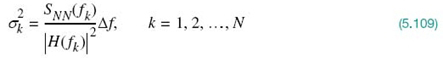
where SN(fk) and |H(fk)| are the noise spectral density and the channel’s magnitude response evaluated at the frequency fk, respectively. The information capacity of the kth subchannel is
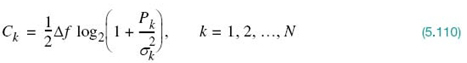
where the factor 1/2 accounts for the fact that Δƒ applies to both positive and negative frequencies. All the N subchannels are independent of one another. Hence, the total capacity of the overall channel is approximately given by the summation

The problem we have to address is to maximize the overall information capacity C subject to the constraint

The usual procedure to solve a constrained optimization problem is to use the method of Lagrange multipliers (see Appendix D for a discussion of this method). To proceed with this optimization, we first define an objective function that incorporates both the information capacity C and the constraint (i.e., (5.111) and (5.112)), as shown by

where λ is the Lagrange multiplier. Next, differentiating the objective function J(Pk) with respect to Pk and setting the result equal to zero, we obtain
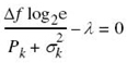
To satisfy this optimizing solution, we impose the following requirement:
where K is a constant that is the same for all k. The constant K is chosen to satisfy the average power constraint.
Inserting the defining values of (5.108) and (5.109) in the optimizing condition of (5.114), simplifying, and rearranging terms we get
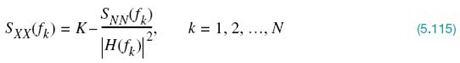
Let ![]() denote the frequency range for which the constant K satisfies the condition
denote the frequency range for which the constant K satisfies the condition

Then, as the incremental frequency interval Δƒ is allowed to approach zero and the number of subchannels N goes to infinity, we may use (5.115) to formally state that the power spectral density of the input ensemble that achieves the optimum information capacity is a nonnegative quantity defined by
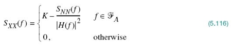
Because the average power of a random process is the total area under the curve of the power spectral density of the process, we may express the average power of the channel input x(t) as
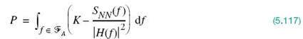
For a prescribed P and specified SN(f) and H(f), the constant K is the solution to (5.117).
The only thing that remains for us to do is to find the optimum information capacity. Substituting the optimizing solution of (5.114) into (5.111) and then using the defining values of (5.108) and (5.109), we obtain
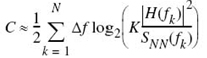
When the incremental frequency interval Δƒ is allowed to approach zero, this equation takes the limiting form
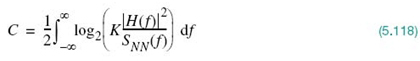
where the constant K is chosen as the solution to (5.117) for a prescribed input signal power P.
Water-filling Interpretation of the Information Capacity Law
Equations (5.116) and (5.117) suggest the picture portrayed in Figure 5.19. Specifically, we make the following observations:
- The appropriate input power spectral density SX(f) is described as the bottom regions of the function SN(f)/|H(f)|2 that lie below the constant level K, which are shown shaded.
- The input power P is defined by the total area of these shaded regions.
The spectral-domain picture portrayed here is called the water-filling (pouring) interpretation, in the sense that the process by which the input power is distributed across the function SN(f)/ |H(f)|2 is identical to the way in which water distributes itself in a vessel.
Consider now the idealized case of a band-limited signal in AWGN channel of power spectral density N(f) = N0/2. The transfer function H(f) is that of an ideal band-pass filter defined by

where fc is the midband frequency and B is the channel bandwidth. For this special case, (5.117) and (5.118) reduce respectively to
![]()
and
![]()
Hence, eliminating K between these two equations, we get the standard form of Shannon’s capacity theorem, defined by (5.95).
EXAMPLE 11 Capacity of NEXT-Dominated Channel
Digital subscriber lines (DSLs) refer to a family of different technologies that operate over a closed transmission loop; they will be discussed in Chapter 8, Section 8.11. For the present, it suffices to say that a DSL is designed to provide for data transmission between a user terminal (e.g., computer) and the central office of a telephone company. A major channel impairment that arises in the deployment of a DSL is the near-end cross-talk (NEXT). The power spectral density of this crosstalk may be taken as

Figure 5.19 Water-filling interpretation of information-capacity theorem for a colored noisy channel.
where SX(f) is the power spectral density of the transmitted signal and HNEXT(f) is the transfer function that couples adjacent twisted pairs. The only constraint we have to satisfy in this example is that the power spectral density function SX(f) be nonnegative for all f. Substituting (5.119) into (5.116), we readily find that this condition is satisfied by solving for K as
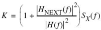
Finally, using this result in (5.118), we find that the capacity of the NEXT-dominated digital subscriber channel is given by

where ![]() is the set of positive and negative frequencies for which SX(f) > 0.
is the set of positive and negative frequencies for which SX(f) > 0.
5.13 Rate Distortion Theory
In Section 5.3 we introduced the source-coding theorem for a discrete memoryless source, according to which the average codeword length must be at least as large as the source entropy for perfect coding (i.e., perfect representation of the source). However, in many practical situations there are constraints that force the coding to be imperfect, thereby resulting in unavoidable distortion. For example, constraints imposed by a communication channel may place an upper limit on the permissible code rate and, therefore, on average codeword length assigned to the information source. As another example, the information source may have a continuous amplitude as in the case of speech, and the requirement is to quantize the amplitude of each sample generated by the source to permit its representation by a codeword of finite length as in pulse-code modulation to be discussed in Chapter 6. In such cases, the problem is referred to as source coding with a fidelity criterion, and the branch of information theory that deals with it is called rate distortion theory.16 Rate distortion theory finds applications in two types of situations:
- Source coding where the permitted coding alphabet cannot exactly represent the information source, in which case we are forced to do lossy data compression.
- Information transmission at a rate greater than channel capacity.
Accordingly, rate distortion theory may be viewed as a natural extension of Shannon’s coding theorem.
Rate Distortion Function
Consider a discrete memoryless source defined by an M-ary alphabet ![]() : {xi|i = 1,2,…,M}, which consists of a set of statistically independent symbols together with the associated symbol probabilities {pi|i = 1,2,…,M}. Let R be the average code rate in bits per codeword. The representation codewords are taken from another alphabet
: {xi|i = 1,2,…,M}, which consists of a set of statistically independent symbols together with the associated symbol probabilities {pi|i = 1,2,…,M}. Let R be the average code rate in bits per codeword. The representation codewords are taken from another alphabet ![]() :{yj| j = 1,2,…,N}. The source-coding theorem states that this second alphabet provides a perfect representation of the source provided that R > H, where H is the source entropy. But if we are forced to have R < H, then there is unavoidable distortion and, therefore, loss of information.
:{yj| j = 1,2,…,N}. The source-coding theorem states that this second alphabet provides a perfect representation of the source provided that R > H, where H is the source entropy. But if we are forced to have R < H, then there is unavoidable distortion and, therefore, loss of information.
Let p(xi, yj) denote the joint probability of occurrence of source symbol xi and representation symbol yj. From probability theory, we have
where p(yj|xi) is a transition probability. Let d(xi, yj) denote a measure of the cost incurred in representing the source symbol xi by the symbol yj; the quantity d(xi, yj) is referred to as a single-letter distortion measure. The statistical average of d(xi, yj) over all possible source symbols and representation symbols is given by
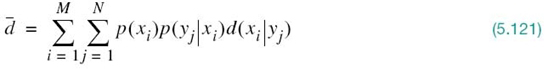
Note that the average distortion ![]() is a nonnegative continuous function of the transition probabilities p(yj|xi) that are determined by the source encoder–decoder pair.
is a nonnegative continuous function of the transition probabilities p(yj|xi) that are determined by the source encoder–decoder pair.
A conditional probability assignment p(yj|xi) is said to be D-admissible if, and only if, the average distortion ![]() is less than or equal to some acceptable value D. The set of all D-admissible conditional probability assignments is denoted by
is less than or equal to some acceptable value D. The set of all D-admissible conditional probability assignments is denoted by
For each set of transition probabilities, we have a mutual information
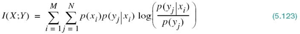
A rate distortion function R(D) is defined as the smallest coding rate possible for which the average distortion is guaranteed not to exceed D. Let ![]() denote the set to which the conditional probability p(yj|xi) belongs for a prescribed D. Then, for a fixed D we write17
denote the set to which the conditional probability p(yj|xi) belongs for a prescribed D. Then, for a fixed D we write17

subject to the constraint
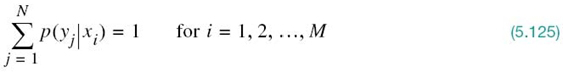
The rate distortion function R(D) is measured in units of bits if the base-2 logarithm is used in (5.123). Intuitively, we expect the distortion D to decrease as the rate distortion function R(D) is increased. We may say conversely that tolerating a large distortion D permits the use of a smaller rate for coding and/or transmission of information.

Figure 5.20 Summary of rate distortion theory.
Figure 5.20 summarizes the main parameters of rate distortion theory. In particular, given the source symbols {xi} and their probabilities {pi}, and given a definition of the single-letter distortion measure d(xi, yj), the calculation of the rate distortion function R(D) involves finding the conditional probability assignment p(yj|xi) subject to certain constraints imposed on p(yj|xi). This is a variational problem, the solution of which is unfortunately not straightforward in general.
EXAMPLE 12 Gaussian Source
Consider a discrete-time, memoryless Gaussian source with zero mean and variance σ2. Let x denote the value of a sample generated by such a source. Let y denote a quantized version of x that permits a finite representation of it. The square-error distortion
![]()
provides a distortion measure that is widely used for continuous alphabets. The rate distortion function for the Gaussian source with square-error distortion, as described herein, is given by
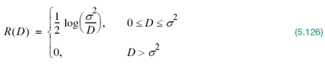
In this case, we see that R(D) → ∞ as D → 0, and R(D) = 0 for D = σ2.
EXAMPLE 13 Set of Parallel Gaussian Sources
Consider next a set of N independent Gaussian random variables ![]() , where Xi has zero mean and variance
, where Xi has zero mean and variance ![]() . Using the distortion measure
. Using the distortion measure
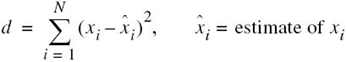
and building on the result of Example 12, we may express the rate distortion function for the set of parallel Gaussian sources described here as
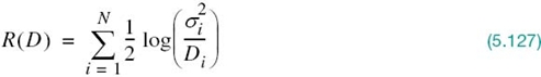
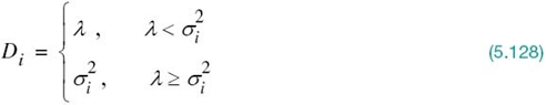
and the constant λ is chosen so as to satisfy the condition
Compared to Figure 5.19, (5.128) and (5.129) may be interpreted as a kind of “water-filling in reverse, ” as illustrated in Figure 5.21. First, we choose a constant λ and only the subset of random variables whose variances exceed the constant λ, No bits are used to describe the remaining subset of random variables whose variances are less than the constant λ.
Figure 5.21 Reverse water-filling picture for a set of parallel Gaussian processes.
5.14 Summary and Discussion
In this chapter we established two fundamental limits on different aspects of a communication system, which are embodied in the source-coding theorem and the channel-coding theorem.
The source-coding theorem, Shannon’s first theorem, provides the mathematical tool for assessing data compaction; that is, lossless compression of data generated by a discrete memoryless source. The theorem teaches us that we can make the average number of binary code elements (bits) per source symbol as small as, but no smaller than, the entropy of the source measured in bits. The entropy of a source is a function of the probabilities of the source symbols that constitute the alphabet of the source. Since entropy is a measure of uncertainty, the entropy is maximum when the associated probability distribution generates maximum uncertainty.
The channel-coding theorem, Shannon’s second theorem, is both the most surprising and the single most important result of information theory. For a binary symmetric channel, the channel-coding theorem teaches us that, for any code rate r less than or equal to the channel capacity C, codes do exist such that the average probability of error is as small as we want it. A binary symmetric channel is the simplest form of a discrete memoryless channel. It is symmetric, because the probability of receiving symbol 1 if symbol 0 is sent is the same as the probability of receiving symbol 0 if symbol 1 is sent. This probability, the probability that an error will occur, is termed a transition probability. The transition probability p is determined not only by the additive noise at the channel output, but also by the kind of receiver used. The value of p uniquely defines the channel capacity C.
The information capacity law, an application of the channel-coding theorem, teaches us that there is an upper limit to the rate at which any communication system can operate reliably (i.e., free of errors) when the system is constrained in power. This maximum rate, called the information capacity, is measured in bits per second. When the system operates at a rate greater than the information capacity, it is condemned to a high probability of error, regardless of the choice of signal set used for transmission or the receiver used for processing the channel output.
When the output of a source of information is compressed in a lossless manner, the resulting data stream usually contains redundant bits. These redundant bits can be removed by using a lossless algorithm such as Huffman coding or the Lempel–Ziv algorithm for data compaction. We may thus speak of data compression followed by data compaction as two constituents of the dissection of source coding, which is so called because it refers exclusively to the sources of information.
We conclude this chapter on Shannon’s information theory by pointing out that, in many practical situations, there are constraints that force source coding to be imperfect, thereby resulting in unavoidable distortion. For example, constraints imposed by a communication channel may place an upper limit on the permissible code rate and, therefore, average codeword length assigned to the information source. As another example, the information source may have a continuous amplitude, as in the case of speech, and the requirement is to quantize the amplitude of each sample generated by the source to permit its representation by a codeword of finite length, as in pulse-code modulation discussed in Chapter 6. In such cases, the information-theoretic problem is referred to as source coding with a fidelity criterion, and the branch of information theory that deals with it is called rate distortion theory, which may be viewed as a natural extension of Shannon’s coding theorem.
Problems
Entropy
5.1 Let p denote the probability of some event. Plot the amount of information gained by the occurrence of this event for 0 ≤ p ≤ 1.
5.2 A source emits one of four possible symbols during each signaling interval. The symbols occur with the probabilities
p0 = 0.4
p1 = 0.3
p2 = 0.2
p3 = 0.1
which sum to unity as they should. Find the amount of information gained by observing the source emitting each of these symbols.
5.3 A source emits one of four symbols s0, s1, s2, and s3 with probabilities 1/3, 1/6, 1/4 and 1/4, respectively. The successive symbols emitted by the source are statistically independent. Calculate the entropy of the source.
5.4 Let X represent the outcome of a single roll of a fair die. What is the entropy of X?
5.5 The sample function of a Gaussian process of zero mean and unit variance is uniformly sampled and then applied to a uniform quantizer having the input–output amplitude characteristic shown in Figure P5.5. Calculate the entropy of the quantizer output.
5.6 Consider a discrete memoryless source with source alphabet S = {s0, s1,…,sK – 1} and source statistics {p0, p1,…,pK – 1}. The nth extension of this source is another discrete memoryless source with source alphabet S(n) = {σ0, σ1,…,σM – 1}, where M = Kn. Let P(σi) denote the probability of σi.
a. Show that, as expected,

b. Show that
where pik is the probability of symbol sik and H(S) is the entropy of the original source.
c. Hence, show that

5.7 Consider a discrete memoryless source with source alphabet S = {s0, s1, s2} and source statistics {0.7, 0.15, 0.15}.
a. Calculate the entropy of the source.
b. Calculate the entropy of the second-order extension of the source.
5.8 It may come as a surprise, but the number of bits needed to store text is much less than that required to store its spoken equivalent. Can you explain the reason for this statement?
5.9 Let a discrete random variable X assume values in the set {x1,x2,…,xn}. Show that the entropy of X satisfies the inequality
H(X) ≤ log n
and with equality if, and only if, the probability pi = 1/n for all i.
Lossless Data Compression
5.10 Consider a discrete memoryless source whose alphabet consists of K equiprobable symbols.
a. Explain why the use of a fixed-length code for the representation of such a source is about as efficient as any code can be.
b. What conditions have to be satisfied by K and the codeword length for the coding efficiency to be 100%?
5.11 Consider the four codes listed below:

a. Two of these four codes are prefix codes. Identify them and construct their individual decision trees.
b.Apply the Kraft inequality to codes I, II, III, and IV. Discuss your results in light of those obtained in part a.
5.12 Consider a sequence of letters of the English alphabet with their probabilities of occurrence
| Letter | a | i | l | m | n | o | p | y |
| Probability | 0.1 | 0.1 | 0.2 | 0.1 | 0.1 | 0.2 | 0.1 | 0.1 |
Compute two different Huffman codes for this alphabet. In one case, move a combined symbol in the coding procedure as high as possible; in the second case, move it as low as possible. Hence, for each of the two codes, find the average codeword length and the variance of the average codeword length over the ensemble of letters. Comment on your results.
5.13 A discrete memoryless source has an alphabet of seven symbols whose probabilities of occurrence are as described here:
| Symbol | s0 | s1 | s2 | s3 | s4 | s5 | s6 |
| Probability | 0.25 | 0.25 | 0.125 | 0.125 | 0.125 | 0.0625 | 0.0625 |
Compute the Huffman code for this source, moving a “combined” symbol as high as possible. Explain why the computed source code has an efficiency of 100%.
5.14 Consider a discrete memoryless source with alphabet {s0, s1, s2} and statistics {0.7, 0.15, 0.15} for its output.
a. Apply the Huffman algorithm to this source. Hence, show that the average codeword length of the Huffman code equals 1.3 bits/symbol.
b. Let the source be extended to order two. Apply the Huffman algorithm to the resulting extended source and show that the average codeword length of the new code equals 1.1975 bits/symbol.
c. Extend the order of the extended source to three and reapply the Huffman algorithm; hence, calculate the average codeword length.
d. Compare the average codeword length calculated in parts b and c with the entropy of the original source.
5.15 Figure P5.15 shows a Huffman tree. What is the codeword for each of the symbols A, B, C, D, E, F, and G represented by this Huffman tree? What are their individual codeword lengths?
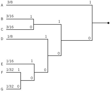
5.16 A computer executes four instructions that are designated by the codewords (00, 01, 10, 11). Assuming that the instructions are used independently with probabilities (1/2, 1/8, 1/8, 1/4), calculate the percentage by which the number of bits used for the instructions may be reduced by the use of an optimum source code. Construct a Huffman code to realize the reduction.
5.17 Consider the following binary sequence
11101001100010110100…
Use the Lempel–Ziv algorithm to encode this sequence, assuming that the binary symbols 0 and 1 are already in the cookbook.
Binary Symmetric Channel
5.18 Consider the transition probability diagram of a binary symmetric channel shown in Figure 5.8. The input binary symbols 0 and 1 occur with equal probability. Find the probabilities of the binary symbols 0 and 1 appearing at the channel output.
5.19 Repeat the calculation in Problem 5.18, assuming that the input binary symbols 0 and 1 occur with probabilities 1/4 and 3/4, respectively.
Mutual Information and Channel Capacity
5.20 Consider a binary symmetric channel characterized by the transition probability p. Plot the mutual information of the channel as a function of p1, the a priori probability of symbol 1 at the channel input. Do your calculations for the transition probability p = 0, 0.1, 0.2, 0.3, 0.5.
5.21 Revisiting (5.12), express the mutual information I(X;Y) in terms of the relative entropy
D(p(x, y)||p(x)p(y))
5.22 Figure 5.10 depicts the variation of the channel capacity of a binary symmetric channel with the transition probability p. Use the results of Problem 5.19 to explain this variation.
5.23 Consider the binary symmetric channel described in Figure 5.8. Let p0 denote the probability of sending binary symbol x0 = 0 and let p1 = 1 – p0 denote the probability of sending binary symbol x1 = 1. Let p denote the transition probability of the channel.
a. Show that the mutual information between the channel input and channel output is given by
![]()
where the two entropy functions
and
![]()
b. Show that the value of p0 that maximizes I(X;Y) is equal to 1/2.
c. Hence, show that the channel capacity equals
C = 1 – H(p)
5.24 Two binary symmetric channels are connected in cascade as shown in Figure P5.24. Find the overall channel capacity of the cascaded connection, assuming that both channels have the same transition probability diagram of Figure 5.8.

5.25 The binary erasure channel has two inputs and three outputs as described in Figure P5.25. The inputs are labeled 0 and 1 and the outputs are labeled 0, 1, and e. A fraction α of the incoming bits is erased by the channel. Find the capacity of the channel.

5.26 Consider a digital communication system that uses a repetition code for the channel encoding/decoding. In particular, each transmission is repeated n times, where n = 2m + 1 is an odd integer. The decoder operates as follows. If in a block of n received bits the number of 0s exceeds the number of 1s, then the decoder decides in favor of a 0; otherwise, it decides in favor of a 1. An error occurs when m + 1 or more transmissions out of n = 2m + 1 are incorrect. Assume a binary symmetric channel.
a. For n = 3, show that the average probability of error is given by
![]()
where p is the transition probability of the channel.
b. For n = 5, show that the average probability of error is given by
![]()
c. Hence, for the general case, deduce that the average probability of error is given by
5.27 Let X, Y, and Z be three discrete random variables. For each value of the random variable Z, represented by sample z, define
![]()
Show that the conditional entropy H(X | Y) satisfies the inequality
![]()
where ![]() is the expectation operator.
is the expectation operator.
5.28 Consider two correlated discrete random variables X and Y, each of which takes a value in the set ![]() . Suppose that the value taken by Y is known. The requirement is to guess the value of X. Let Pe denote the probability of error, defined by
. Suppose that the value taken by Y is known. The requirement is to guess the value of X. Let Pe denote the probability of error, defined by
![]()
Show that Pe is related to the conditional entropy of X given Y by the inequality
![]()
This inequality is known as Fano’s inequality. Hint: Use the result derived in Problem 5.27.
5.29 In this problem we explore the convexity of the mutual information I(X;Y), involving the pair of discrete random variables X and Y.
Consider a discrete memoryless channel, for which the transition probability p(y|x) is fixed for all x and y. Let X1 and X2 be two input random variables, whose input probability distributions are respectively denoted by p(x1) and p(x2). The corresponding probability distribution of X is defined by the convex combination
p(x) = a1p(x1) + a2 p(x2)
where a1 and a2 are arbitrary constants. Prove the inequality
I(X;Y) ≥ a1I(X1;Y1) + a2I(X2;Y2)
where X1, X2, and X are the channel inputs, and Y1, Y2, and Y are the corresponding channel outputs. For the proof, you may use the following form of Jensen’s inequality:

Differential Entropy
5.30 The differential entropy of a continuous random variable X is defined by the integral of (5.66). Similarly, the differential entropy of a continuous random vector X is defined by the integral of (5.68). These two integrals may not exist. Justify this statement.
5.31 Show that the differential entropy of a continuous random variable X is invariant to translation; that is,
h(X + c) = h(X)
for some constant c.
5.32 Let X1, X2,…,Xn denote the elements of a Gaussian vector X. The Xi are independent with mean miand variance ![]() , i = 1,2,…,n. Show that the differential entropy of the vector X is given by
, i = 1,2,…,n. Show that the differential entropy of the vector X is given by
![]()
where e is the base of the natural logarithm. What does h(X) reduce to if the variances are all equal?
5.33 A continuous random variable X is constrained to a peak magnitude M; that is,
–M < X < M
a. Show that the differential entropy of X is maximum when it is uniformly distributed, as shown by
b. Determine the maximum differential entropy of X.
5.34 Referring to (5.75), do the following:
a. Verify that the differential entropy of a Gaussian random variable of mean μ and variance σ2 is given by 1/2 log2(2π e σ2), where e is the base of the natural algorithm.
b. Hence, confirm the inequality of (5.75).
5.35 Demonstrate the properties of symmetry, nonnegativity, and expansion of the mutual information I(X;Y) described in Section 5.6.
5.36 Consider the continuous random variable Y, defined by
Y = X + N
where the random variables X and N are statistically independent. Show that the conditional differential entropy of Y, given X, equals
h(Y | X) = h(N)
where h(N) is the differential entropy of N.
Information Capacity Law
5.37 A voice-grade channel of the telephone network has a bandwidth of 3.4 kHz.
a. Calculate the information capacity of the telephone channel for a signal-to-noise ratio of 30 dB.
b. Calculate the minimum signal-to-noise ratio required to support information transmission through the telephone channel at the rate of 9600 bits/s.
5.38 Alphanumeric data are entered into a computer from a remote terminal through a voice-grade telephone channel. The channel has a bandwidth of 3.4 kHz and output signal-to-noise ratio of 20 dB. The terminal has a total of 128 symbols. Assume that the symbols are equiprobable and the successive transmissions are statistically independent.
a. Calculate the information capacity of the channel.
b. Calculate the maximum symbol rate for which error-free transmission over the channel is possible.
5.39 A black-and-white television picture may be viewed as consisting of approximately 3 × 10⁵ elements, each of which may occupy one of 10 distinct brightness levels with equal probability. Assume that (1) the rate of transmission is 30 picture frames per second and (2) the signal-to-noise ratio is 30 dB.
Using the information capacity law, calculate the minimum bandwidth required to support the transmission of the resulting video signal.
5.40 In Section 5.10 we made the statement that it is easier to increase the information capacity of a communication channel by expanding its bandwidth B than increasing the transmitted power for a prescribed noise variance N0B. This statement assumes that the noise spectral density N0 varies inversely with B. Why is this inverse relationship the case?
5.41 In this problem, we revisit Example 5.10, which deals with coded binary antipodal signaling over an additive white Gaussian noise (AWGN) channel. Starting with (5.105) and the underlying theory, develop a software package for computing the minimum Eb/N0 required for a given bit error rate, where Eb is the signal energy per bit, and N0/2 is the noise spectral density. Hence, compute the results plotted in parts a and b of Figure 5.16.
As mentioned in Example 5.10, the computation of the mutual information between the channel input and channel output is well approximated using Monte Carlo integration. To explain how this method works, consider a function g(y) that is difficult to sample randomly, which is indeed the case for the problem at hand. (For this problem, the function g(y) represents the complicated integrand in the formula for the differential entropy of the channel output.) For the computation, proceed as follows:
- Find an area A that includes the region of interest and that is easily sampled.
- Choose N points, uniformly randomly inside the area A.
Then the Monte Carlo integration theorem states that the integral of the function g(y) with respect to y is approximately equal to the area A multiplied by the fraction of points that reside below the curve of g, as illustrated in Figure P5.41. The accuracy of the approximation improves with increasing N.

Notes
1. According to Lucky (1989), the first mention of the term information theory by Shannon occurred in a 1945 memorandum entitled “A mathematical theory of cryptography.” It is rather curious that the term was never used in Shannon’s (1948) classic paper, which laid down the foundations of information theory. For an introductory treatment of information theory, see Part 1 of the book by McEliece (2004), Chapters 1–6. For an advanced treatment of this subject, viewed in a rather broad context and treated with rigor, and clarity of presentation, see Cover and Thomas (2006).
For a collection of papers on the development of information theory (including the 1948 classic paper by Shannon), see Slepian (1974). For a collection of the original papers published by Shannon, see Sloane and Wyner (1993).
2. The use of a logarithmic measure of information was first suggested by Hartley (1928); however, Hartley used logarithms to base 10.
3. In statistical physics, the entropy of a physical system is defined by (Rief, 1965: 147)
![]()
where kB is Boltzmann’s constant, Ω is the number of states accessible to the system, and ln denotes the natural logarithm. This entropy has the dimensions of energy, because its definition involves the constant kB. In particular, it provides a quantitative measure of the degree of randomness of the system. Comparing the entropy of statistical physics with that of information theory, we see that they have a similar form.
4. For the original proof of the source coding theorem, see Shannon (1948). A general proof of the source coding theorem is also given in Cover and Thomas (2006). The source coding theorem is also referred to in the literature as the noiseless coding theorem, noiseless in the sense that it establishes the condition for error-free encoding to be possible.
5. For proof of the Kraft inequality, see Cover and Thomas (2006). The Kraft inequality is also referred to as the Kraft–McMillan inequality in the literature.
6. The Huffman code is named after its inventor D.A. Huffman (1952). For a detailed account of Huffman coding and its use in data compaction, see Cover and Thomas (2006).
7. The original papers on the Lempel–Ziv algorithm are Ziv and Lempel (1977, 1978). For detailed treatment of the algorithm, see Cover and Thomas (2006).
8. It is also of interest to note that once a “parent” subsequence is joined by its two children, that parent subsequence can be replaced in constructing the Lempel–Ziv algorithm. To illustrate this nice feature of the algorithm, suppose we have the following example sequence:
01, 010, 011,…
where 01 plays the role of a parent and 010 and 011 play the roles of the parent’s children. In this example, the algorithm removes the 01, thereby reducing the length of the table through the use of a pointer.
9. In Cover and Thomas (2006), it is proved that the two-stage method, where the source coding and channel coding are considered separately as depicted in Figure 5.11, is as good as any other method of transmitting information across a noisy channel. This result has practical implications, in that the design of a communication system may be approached in two separate parts: source coding followed by channel coding. Specifically, we may proceed as follows:
- Design a source code for the most efficient representation of data generated by a discrete memoryless source of information.
- Separately and independently, design a channel code that is appropriate for a discrete memoryless channel.
The combination of source coding and channel coding designed in this manner will be as efficient as anything that could be designed by considering the two coding problems jointly.
10. To prove the channel-coding theorem, Shannon used several ideas that were new at the time; however, it was some time later when the proof was made rigorous (Cover and Thomas, 2006: 199). Perhaps the most thoroughly rigorous proof of this basic theorem of information theory is presented in Chapter 7 of the book by Cover and Thomas (2006). Our statement of the theorem, though slightly different from that presented by Cover and Thomas, in essence is the same.
11. In the literature, the relative entropy is also referred to as the Kullback–Leibler divergence (KLD).
12. Equation (5.95) is also referred to in the literature as the Shannon–Hartley law in recognition of the early work by Hartley on information transmission (Hartley, 1928). In particular, Hartley showed that the amount of information that can be transmitted over a given channel is proportional to the product of the channel bandwidth and the time of operation.
13. A lucid exposition of sphere packing is presented in Cover and Thomas (2006); see also Wozencraft and Jacobs (1965).
14. Parts a and b of Figure 5.16 follow the corresponding parts of Figure 6.2 in the book by Frey (1998).
15. For a rigorous treatment of information capacity of a colored noisy channel, see Gallager (1968). The idea of replacing the channel model of Figure 5.17a with that of Figure 5.17b is discussed in Gitlin, Hayes, and Weinstein (1992)
16. For a complete treatment of rate distortion theory, see the classic book by Berger (1971); this subject is also treated in somewhat less detail in Cover and Thomas (1991), McEliece (1977), and Gallager (1968).
17. For the derivation of (5.124), see Cover and Thomas (2006). An algorithm for computation of the rate distortion function R(D) defined in (5.124) is described in Blahut (1987) and Cover and Thomas (2006).